| Issue |
A&A
Volume 661, May 2022
|
|
|---|---|---|
| Article Number | A74 | |
| Number of page(s) | 22 | |
| Section | Catalogs and data | |
| DOI | https://doi.org/10.1051/0004-6361/202142973 | |
| Published online | 17 May 2022 | |
IBIS-A: The IBIS data Archive
High-resolution observations of the solar photosphere and chromosphere with contextual data★
1
INAF–Osservatorio Astronomico di Roma,
via Frascati 33,
00078
Monte Porzio Catone,
Italy
e-mail: This email address is being protected from spambots. You need JavaScript enabled to view it.
2
ASI Agenzia Spaziale Italiana,
via della Ricerca Scientifica,
Roma,
Italy
3
INAF–Osservatorio Astronomico di Trieste,
Via Giambattista Tiepolo, 11,
34131
Trieste,
Italy
4
INAF–Osservatorio Astrofisico di Catania,
Via S. Sofia 78,
95123
Catania,
Italy
5
INAF–Osservatorio Astrofisico di Arcetri,
Largo Enrico Fermi 5,
50125
Firenze,
Italy
6
National Solar Observatory,
3665 Discovery Drive,
Boulder
CO
80303,
USA
Received:
21
December
2021
Accepted:
4
February
2022
Abstract
Context. The IBIS data Archive (IBIS-A) stores data acquired with the Interferometric BIdimensional Spectropolarimeter (IBIS), which was operated at the Dunn Solar Telescope of the US National Solar Observatory from June 2003 to June 2019. The instrument provided series of high-resolution narrowband spectropolarimetric imaging observations of the photosphere and chromosphere in the range 5800–8600 Å and co-temporal broadband observations in the same spectral range and with the same field of view as for the polarimetric data.
Aims. We present the data currently stored in IBIS-A, as well as the interface utilized to explore such data and facilitate its scientific exploitation. To this end, we also describe the use of IBIS-A data in recent and undergoing studies relevant to solar physics and space weather research.
Methods. IBIS-A includes raw and calibrated observations, as well as science-ready data. The latter comprise maps of the circular, linear, and net circular polarization, and of the magnetic and velocity fields derived for a significant fraction of the series available in the archive. IBIS-A furthermore contains links to observations complementary to the IBIS data, such as co-temporal high-resolution observations of the solar atmosphere available from the instruments onboard the Hinode and IRIS satellites, and full-disk multi-band images from INAF solar telescopes.
Results. IBIS-A currently consists of 30 TB of data taken with IBIS during 28 observing campaigns performed in 2008 and from 2012 to 2019 on 159 days. Of the observations, 29% are released as Level 1 data calibrated for instrumental response and compensated for residual seeing degradation, while 10% of the calibrated data are also available as Level 1.5 format as multi-dimensional arrays of circular, linear, and net circular polarization maps, and line-of-sight velocity patterns; 81% of the photospheric calibrated series present Level 2 data with the view of the magnetic and velocity fields of the targets, as derived from data inversion with the Very Fast Inversion of the Stokes Vector code. Metadata and movies of each calibrated and science-ready series are also available to help users evaluate observing conditions.
Conclusions. IBIS-A represents a unique resource for investigating the plasma processes in the solar atmosphere and the solar origin of space weather events. The archive currently contains 454 different series of observations. A recently undertaken effort to preserve IBIS observations is expected to lead in the future to an increase in the raw measurements and the fraction of processed data available in IBIS-A.
Key words: Sun: atmosphere / Sun: photosphere / Sun: chromosphere / methods: data analysis / astronomical databases: miscellaneous
Research supported by the H2020 SOLARNET grant no. 824135.
e-mail: This email address is being protected from spambots. You need JavaScript enabled to view it.
© ESO 2022
1 Introduction
The solar atmosphere is a highly structured, complex, and strongly dynamic environment produced by the continuous interplay between unmagnetized and magnetized plasmas that permeate it (e.g., Rempel & Schlichenmaier 2011; Stein 2012; Cheung & Isobe 2014; van Driel-Gesztelyi & Green 2015; Bellot Rubio & Orozco Suárez 2019; Wiegelmann & Sakurai 2021). This interplay drives the Sun’s activity and radiative variability on timescales from seconds to centuries. In addition, it imposes electromagnetic forces in the whole heliosphere by modulating the solar particulate and magnetic flux (e.g., Kilpua et al. 2017; Temmer 2021). The same interplay also plays a fundamental role in hugely diverse astrophysical systems. For example, in addition to being responsible for the evolution of magnetic features, coronal heating, and wind acceleration in the solar and stellar atmospheres (e.g., Schmelz 2003), it is responsible for the acceleration of jets from active galactic nuclei and gamma ray bursts (e.g., Blandford et al. 2019) and for the heating of the warm-ionized medium of galaxies (e.g., Padoan & Nordlund 2011). In all these systems unmagnetized and magnetized plasmas interrelate on small spatial and temporal scales that are still beyond those achievable with current telescopes. However, these scales will be accessible soon in the Sun’s atmosphere with the upcoming 4 m class solar telescopes such as the National Science Foundation’s Daniel K. Inouye Solar Telescope (DKIST, Rimmele et al. 2020; Rast et al. 2021) and the European * Solar Telescope (EST, Collados et al. 2013; Schlichenmaier et al. 2019).
Nevertheless, analysis of high-resolution multi-wavelength spectropolarimetric observations of the Sun’s atmosphere performed over the past two decades have already yielded a wealth of information on the interaction between unmagnetized and magnetized plasmas (e.g., van Driel-Gesztelyi & Green 2015; Jess et al. 2015; Borrero et al. 2017; Bellot Rubio & Orozco Suárez 2019). These observations include data acquired with the Interferometric BIdimensional Spectrometer (IBIS, Cavallini 2006), which combined dual tunable Fabry-Perot interferometers with a high-order adaptive optics system and short exposures, to perform high-resolution solar studies.
IBIS was developed at the INAF Arcetri Astrophysical Observatory with contributions from the Universities of Florence and Rome Tor Vergata. It was installed at the Dunn Solar Telescope (DST) of the National Solar Observatory (NSO) in New Mexico (USA) in June 2003, on an optical bench fed by a high-order adaptive optics system. It was operated there by INAF and NSO from 2005 to 2019 as a facility instrument. In 2019 the instrument was dismantled for refurbishing in light of its reinstallation at a different telescope (Ermolli et al. 2020).
From 2003 to 2019 IBIS provided data of the solar photosphere and chromosphere at high spectral, spatial, and temporal resolution over a relatively large field of view (FOV); more details are presented in Sect. 2.2. These data were often acquired simultaneously to those from other instruments installed at the DST, for example the Rapid Oscillations in the Solar Atmosphere (ROSA, Jess et al. 2010) and the Facility Infrared Spectrometer (FIRS, Jaeggli et al. 2012). In addition, IBIS often observed co-temporally with other instruments in the framework of coordinated observing campaigns with space-borne telescopes, for example the Solar and Heliospheric Observatory/Michelson Doppler Imager (SOHO/MDI, Scherrer et al. 1995), Hinode/Solar Optical Telescope (Hinode/SOT, Tsuneta et al. 2008), Solar Dynamics Observatory/Helioseismic and Magnetic Imager (SDO/HMI, Scherrer et al. 2012), SDO/Atmospheric Imaging Assembly (SDO/AIA, Lemen et al. 2012), Interface Region Imaging Spectrograph (IRIS, De Pontieu et al. 2014), and ground-based telescopes, such as the New Solar Telescope (NST, Cao et al. 2010) and Atacama Large Millimeter/submillimeter Array (ALMA, Wedemeyer et al. 2020). With the DST located in the mountains above the White Sands Missile Range, IBIS also co-observed with many solar sounding rocket payloads launched from the range, including the Extreme Ultraviolet Normal Incidence Spectrograph (EUNIS, Brosius et al. 2014), High Resolution Coronal Imager (Hi-C, Kobayashi et al. 2014), Chromospheric Lyman-Alpha Spectro-Polarimeter (CLASP, Narukage et al. 2016), and Very high Angular resolution Ultraviolet Telescope (VAULT, Vourlidas et al. 2016). Instead, due to different time zones and telescope operations, there are few if any co-temporary observations between IBIS and other spectropolarimetric instruments installed at the solar telescopes on the Canary Islands, for example the CRisp Imaging Spectro-Polarimeter (CRISP, Scharmer et al. 2008) and the CHROMospheric Imaging Spectrometer (CHROMIS, Scharmer et al. 2019) operating at the Swedish 1-m Solar Telescope (SST, Scharmer et al. 2003).
Given the versatility of the instrument, IBIS data have been used to study a variety of topics, including the temporal evolution and 3D nature of plasma flow in quiet regions (Del Moro et al. 2007) and large-scale magnetic features (Giordano et al. 2008; Sobotka et al. 2012, Sobotka et al. 2013); turbulent solar convection (Viavattene et al. 2020, 2021); structure and brightness of small-(Viticchié et al. 2009, 2010; Romano et al. 2012) and large-scale magnetic features (Criscuoli et al. 2012); dissipation of magnetic energy by current sheets above sunspot umbrae (Tritschler et al. 2008); identification, formation, and decay of active regions (Ermolli et al. 2017; Zuccarello et al. 2009; Murabito et al. 2016, 2017; Schilliro & Romano 2021); formation, atmospheric stratification, and brightening in penumbral regions (Romano et al. 2013, Romano et al. 2014, 2020; Murabito et al. 2019, Murabito et al. 2020a); acoustic oscillations and MHD wave propagation in the solar atmosphere (Vecchio et al. 2007, 2009; Stangalini et al. 2011, Stangalini et al. 2012, 2013; Sobotka et al. 2016; Abbasvand et al. 2020; Houston et al. 2020) and in sunspots (Stangalini et al. 2018, Stangalini et al. 2021a,b,c, 2022); First Ionization Potential (FIP) effect (Baker et al. 2021); magnetic flux emergence from the photosphere to the chromosphere (Murabito et al. 2020a); chromospheric vortices (Murabito et al. 2020b); flares (Kowalski et al. 2015; Capparelli et al. 2017; Romano et al. 2017); sensitivity of spectral line diagnostics to temperature variations and small-scale magnetic fields (Criscuoli et al. 2013); and new spectroscopic diagnostics of the solar chromosphere (Cauzzi et al. 2008, 2009; Straus et al. 2008; Reardon et al. 2009; Judge et al. 2010; Lipartito et al. 2014; Molnar et al. 2019).
Recently, an effort has been undertaken to collect the data acquired by the IBIS instrument and to preserve them in the permanent IBIS-Archive (IBIS-A). In this paper we describe the public release of the data available in IBIS-A. We introduce the IBIS observations and their processing in Sect. 2. We present the data available in IBIS-A and their quality in Sect. 3. We give an outline of the data access and examples of unexplored data available in IBIS-A in Sects. 4 and 5, respectively. Finally, we summarize this work and draw our conclusions in Sect. 6.
2 Observations and data processing
2.1 IBIS
The IBIS instrument (Cavallini 2006) basically consisted of two tunable Fabry-Pérot interferometers (FPs) and narrowband interference filters (hereafter pre-filters) operating in a classical mount over the spectral range 5800–8600 Å (later extended to 5400–8600 Å). During operations, the combination of the FPs, pre-filters, and instrument control allowed tuning the instrument transmission in wavelength sequentially through spectral lines isolated by the pre-filters. The number of wavelength points sampled per line, as well as the number of lines used in sequence, were defined by the observer depending on science target and available pre-filters.
It is worth noting that the layout and optical components of the IBIS instrument underwent improvements over time. For example, the addition of a polarimetric unit in 2006 expanded measurements at the spectral positions sampled by the instrument to all the Stokes polarization states (I, Q, U, V). After this upgrade, the instrument also underwent the implementation of new detectors and control software in 2010. However, these changes did not affect the main characteristics of the instrument described above. Moreover, from 2011 to 2019 the instrument had a rather stable condition with only minor modifications that did not significantly change the main characteristics of the data acquired by the instrument.
A thorough evaluation of the optical performance of IBIS is provided by Reardon & Cavallini (2008) and Righini et al. (2010). In brief, the instrument had a transmission profile with a full width at half maximum (FWHM) of 24.0 mÅ at 6328 Å (Reardon & Cavallini 2008) and a pixel scale of 0.082 arcsec per pixel (until 2010) or 0.098 arcsec per pixel (after 2010). These values allowed observations at the diffraction limit of the DST (≈ 0.16 arcsec at 5800 Å). Further details concerning the IBIS data are found in Sect. 2.2.
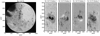 |
Fig. 1 Examples of IBIS data acquired (from left to right) in standard spectroscopic and spectropolarimetric modes at the Fe I 6173 Å line with circular (1000 × 1000 pixels2) and rectangular (350 × 800 pixels2) FOV on 25 October 2014, 15:32 UT and 13 May 2016, 13:38 UT at disk positions μ = 0.85 and μ = 0.68, respectively. The spectroscopic and spectropolarimetric Stokes I observations were taken in the line continuum, while the spectropolarimetric Stokes Q and Stokes U and V data were acquired in the line core and line blue wing, respectively. Shown here are the Level 1 data derived from the instrumental calibrations and MOMFBD restoration (see Sects. 2.2 and 3.1 for more details). |
2.2 Observing campaigns
A typical IBIS dataset consists of measurements taken in sequence over multiple spectral lines (two or three lines, e.g., Fe I at 6302 Å, Fe I at 6173 Å, and Ca II at 8542 Å), with each line sampled at several spectral positions (often between 10 and 30 positions), each position at six polarimetric modulation states (I ± [Q, U, V]), and each state with either a single exposure or multiple exposures. The data are characterized by a high spectral (R > 200000), spatial (≈0.16–0.24 arcsec), and temporal (8–15 frames per second) resolution over a relatively large FOV (minimum linear dimension >40 arcsec; see details in the following). IBIS ensured a high wavelength stability in time of the instrumental profile (with a drift on the order of 10 m s−1 over 10 h), short exposure times to partially freeze the Earth’s atmospheric seeing (tens of ms), and nearly diffraction-limited resolution over the whole FOV.
The instrument could be operated in both the spectroscopic and spectropolarimetric modes. It also allowed for a hybrid mode where full-Stokes measurements were taken in some of the selected spectral lines while only spectral Stokes-I measurements were acquired for other lines. In standard spectroscopic mode the FOV was often circular with a diameter of ≈95 arcsec, as defined by a circular mask inserted in the entrance focal plane of the instrument. In standard spectropolarimetric mode the FOV was rectangular with a dimension of ≈40 × 95 arcsec2, as a result of the rectangular mask inserted in the focal entrance plane of the instrument so that the two orthogonally linear polarized beams could be imaged onto the same detector.
The spectroscopic and spectropolarimetric observational modes were both operated with acquisition of broadband (BB) images simultaneous to the narrowband (NB) data produced by the two FPs. The BB images allow for post-facto compensation of residual seeing degradation with enhancement of the image quality (Löfdahl 2016).
Figure 1 shows examples of IBIS data acquired in the standard spectroscopic and spectropolarimetric observational modes after instrumental calibrations and further processing described in Sect. 2.3. In particular, we show the spectroscopic observation at the photospheric Fe 16173 Å line of a large sunspot region with umbral and penumbral areas imaged near the disk center, and the Stokes-I, -Q, -U, and -V measurements of a smaller sunspot region observed closer to the limb.
2.3 Data processing
IBIS-A includes the camera data originally generated by the instrument, as well as processed data. The latter were obtained with a reduction package built on the IBIS calibration pipeline (Criscuoli & Tritschler 2014) released by NSO1 and with other codes. The NSO pipeline includes calibration for the dark current, for the flat-field response, and for the gain of the detectors; computation of the detector image scale and orientation; compensation for the artificial polarization introduced by the instrumentation and by the telescope; and calibrations for the systematic wavelength shift across the FOV due to the collimated mounting of the FPs and for residual effects of the seeing. In addition, the data available in IBIS-A were calibrated for pre-filter transmission curves and residual polarization crosstalk between Stokes-I and Stokes-Q, -U, -V data. Moreover, the BB data were processed for image restoration by using the outcomes of the Multi-Object Multi-Frame Blind Deconvolution (MOMFBD, Löfdahl 2012; van Noort et al. 2005) in order to enhance the image quality over the full FOV. The package employed to process the data is written in IDL2, and it is run under a Linux Ubuntu distribution. The codes are run in semiautomatic mode, which requires inputs from the user at two steps in order to select the FOV for alignment of NB and BB images and to compute the residual polarization cross-talk. At present the MOMFBD restoration, which is written in C++, is not integrated in the data reduction package.
The IBIS measurements processed for the above steps form the Level 1 data in IBIS-A. At present there are 133 calibrated series out of the 454 series of raw IBIS observations stored in the archive.
A subset of the Level 1 observations was further processed to generate Level 1.5 data. This subset consists of the calibrated spectropolarimetric observations acquired at the photospheric Fe I 6173 Å and chromospheric Ca II 8542 Å lines under homogeneous instrumental setup (i.e., the same observing mode and spectral sampling).
The Level 1.5 data comprise maps of the mean circular polarization (CP), mean linear polarization (LP), and net circular polarization (NCP), and of the line-of-sight (los) velocity field (Vlos). The mean CP signal was estimated via two methods. The first involved computing the maximum amplitude of the Stokes-V spectral profile, as reported in Stangalini et al. (2021a), with the formula
 (1)
(1)
where Vmax is the maximum amplitude of the Stokes-V parameter in the measured profile and Icont the local continuum intensity. In the second method all the values of the Stokes-V profile as set out by Martínez Pillet et al. (2011) are considered. The second method was adapted to account for the actual number n of spectral points sampled during the observations. In particular, we applied the formula
 (2)
(2)
where ϵ = 1 for the spectral positions of the line sampling on the blue wing of the line, ϵ = −1 for the spectral positions on the red wing, and ϵ = 0 for the line center position; n = 21 is the number of sampled spectral positions; and i runs from the 1st to the 21st wavelength position. The values 〈Ic〉 and Vi are the average line continuum intensity in a quiet-Sun region within the FOV and of the Stokes-V parameter at the wavelength position i.
We also estimated the LP signal via the method set out by Martínez Pillet et al. (2011), using the formula
 (3)
(3)
where Qi and Ui are the values of the Stokes-Q and Stokes-U parameters at the wavelength position i.
The NCP, which is a measure of the asymmetry of the Stokes-V polarization signal, was estimated from the integral of the measured Stokes-V profile following Solanki & Montavon (1993). In particular, we applied the formula
 (4)
(4)
where λ, λ1, and λn represent the wavelength, and the wavelengths at the 1st and 21st spectral positions of the sampled line, respectively. We computed Vlos by using the phase cross-correlation of Fourier transform as set out in Sect. 2.4 of Schlichenmaier & Schmidt (2000).
The Level 1.5 data were computed by utilizing the Matplotlib (Hunter 2007), Scipy (Virtanen et al. 2020), and Numpy (Harris et al. 2020) libraries written in Python. At present, there are 14 different series of Level 1.5 data available in the archive.
Finally, the Level 1 series from spectropolarimetric observations at the Fe I 6173 Å line were further considered to generate Level 2 data. In particular, all the scans of the above series were processed with inversion techniques. The core of these techniques relies on the inference of the dynamic, magnetic, and thermodynamic properties of the imaged atmosphere from the measured Stokes profiles of single or multiple spectral lines that form at different heights in the solar atmosphere. This is achieved by solving the radiative transfer equation through codes aimed at working the inverse problem (del Toro Iniesta & Ruiz Cobo 2016). The Level 2 data in IBIS-A were obtained with the Very Fast Inversion of the Stokes Vector code (VFISV, Borrero et al. 2011), version 4.0, which performs a Milne-Eddington inversion of measured Stokes profiles. At present, 31 data series have been inverted and a total of 2902 scans processed, which let more than 80% of the calibrated Fe 16173 Å line observations stored in the archive to also be available as Level 2 data.
The FOV size of Level 1 data3 is 500 × 1000 pixels2, while the science-ready Level 1.5 and 2.0 data both cover 350 × 800 pixels2, or ≈34 × 78 arcsec2.
3 IBIS-A data
The IBIS observing campaigns varied depending on instrumental setup, observer, target, and science goals, thus the acquired data are heterogeneous. However, almost all the IBIS datasets include the sampling of a photospheric line and a chromospheric line, either Ca II 8542 Å or Hα 6563 Å, and sometimes both. From 2013 to 2017 the chromospheric Ca II 8542 Å observations were frequently carried out in spectropolarimetric mode.
Figure 2 summarizes the main characteristics of the IBIS data available in IBIS-A. Figure 2 panels a and b show the fraction of spectroscopic and spectropolarimetric series, and the spectral lines sampled in the observations, respectively. The spectropolarimetric data are 37% of the available measurements (in terms of number of sets). Over 19%, 6%, and 4% of the data refer to the photosphere sampled at the Fe 16173 Å, Fe 16302 Å, and Na I 5896 Å lines, respectively; 38% and 27% of the data report observations of the chromosphere at the Ca II 8542 Å and Hα 6563 Å lines, respectively. Figure 2 panels c and d display the fraction of sequences in the archive depending on their duration and solar disk position of the target, respectively. Almost 56% of the data consist of sequences of observations lasting less than 30 min, but more than 12% of the available data report on long-duration observations exceeding 1 h. In addition, it is worth noting that “duration” in these statistics refers to the length of the individual series. However, sometimes multiple series were run with minimal delay between them, and could thus be considered a continuous observing block. About 53% of the observations were taken at disk center (μ > 0.85, where μ = cosθ and θ is the heliocentric angle), while over 40% of the data image the solar atmosphere at intermediate disk locations (0.25 < μ < 0.85) and about 4% very close to the limb (0.04 < μ < 0.1) or above it.
Figure 3 (top panel) describes the IBIS-A data in terms of the median value of the “quality image” parameter q. This quantity is a measure of the image resolution in arcsec due to the seeing. It is generated by the DST control system by monitoring the variability of the intensity of the Sun’s light during the observing run (see Seykora 1993 for more details). Figure 3 shows that more than 77% of the IBIS-A data were taken under very good and average seeing conditions (i.e., image resolution <1 arcsec), while about 4% of the observations are of the solar atmosphere at medium spatial resolution with image resolution >1.5 arcsec. About 18% of the data are characterized by a resolution in the range 1–1.5 arcsec.
Figure 3 (bottom panel) provides information on the homogeneity of the datasets available in the archive. Here we show the number of datasets depending on the homogeneity of the image quality parameter q during the observing run, for observations of given duration d. The distribution of values in Fig. 3 (bottom panel) shows that a large fraction of the short duration datasets available in IBIS-A were taken under stable excellent and good seeing conditions, but this also holds for a significant number of observations exceeding 1 h.
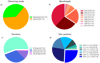 |
Fig. 2 Level 0 data stored in the archive. Shown are pie charts of the fraction (in %) of panel a) the spectroscopic and spectropolarimetric data available in IBIS-A, panel b) the spectral lines (in Å) acquired during the observations, panel c) the duration (in minutes) of the observational sequences, and panel d) the μ disk position of the FOV (μ = cosθ where θ is the heliocentric angle). |
3.1 Data format
IBIS-A includes the data generated by the instrument, those processed for instrumental calibration and seeing restoration, and those further elaborated to derive physical quantities and science-ready data. These diverse sets, which form the Level 0, Level 1, Level 1.5, and Level 2 data, respectively, are stored in the archive with different formats.
The Level 0 data (≈25TB of data) are archived as extended FITS format files in a main folder comprising two subdirectories. These include the NB and BB data, respectively, containing data for both science and instrumental calibrations. The name of the files describes the nature of the data (e.g., Science, Dark, Flat-Field). Each file comprises the data from a single iteration of all pre-filters and wavelengths used during observations. General information about the data, which is common to the whole observing run, is stored in the primary FITS header, while information specific to a single exposure (e.g., acquisition time, wavelength position, exposure time, telescope pointing, polarization state) is stored in the extended FITS headers. Figures A.1 and A.2 give examples of such information. Each FITS file consists of a four-dimensional array with (x, y, λ, Pol)-axes, where the spatial x- and y-axes describe the instrument FOV, the λ-axis covers the wavelength spectral points along the sampled line, and the Pol-axis represents the six polarimetric states (I+Q, I-Q, I+V, I-V, I+U, and I-U) measured by the instrument. The above structure and labeling of the Level 0 data follow the IBIS data definition and file arrangement given at the DST.
Table 1 gives an overview of the Level 0 data currently available in IBIS-A, with information on the number of datasets, and the fraction of observations depending on the target and on sampled spectral lines. The information is provided per year from 2012 to 2019. Table 1 shows that there is a variety of observations at different lines, and targets available in IBIS-A, the latter including quiet Sun, sunspot, pore, and limb regions. Some of the data also relate to plages and filaments.
The Level 1 data (≈4 TB of data) are stored in the archive using the .sav format generated by the IDL pipeline applied to the Level 0 observations. The Level 1 files consist of four-dimensional arrays with (x, y, λ, Stokes)-axes, where the spatial x- and y-axes describe the instrument FOV, the λ-axis renders the wavelength of the line sampling during the observation, and the Stokes-axis represents the (I, Q, U, V) polarimetric states of the measurements. Each Level 1 file also contains information about the data in the info_nb variable, which is a structure with several tags and values. Figure A.3 lists the fields included in the info_nb variable. The Level 1 data are stored with the naming convention llll-nbsss.pc.sav and llll-nbsss.sav for the spectropolarimetric and purely spectroscopic data, respectively, where “llll” is the wavelength (in Å) and “sss” is the scan number in the corresponding Level 0 data. Each .sav file thus reports the data at the given time t of the “sss” scan during the sequence of observations. The structure and naming of the Level 1 data follow those set in the NSO calibration pipeline.
Table A.1 summarizes the main information of the Level 1 data currently available in IBIS-A, with details on targets, lines and number of spectral points sampled during observations, number of measurements at each spectral point, and number of line scans. Table A.1 makes it clear that most of these data currently include observations of the chromosphere at the Ca II 8542 Å and Hα 6563 Å lines. It is worth noting that the Level 1 data of IBIS-A can be accessed with the CRIsp SPectral EXplorer (CRISPEX) graphical user interface (Vissers & Rouppe van der Voort 2012; Löfdahl et al. 2021), version 1.7.4, which was developed to manage the CRISP and CHROMIS data. For this purpose the IBIS data format needs to be adapted to the FITS format accepted by the CRISPEX interface with a code available at the IBIS-A site specified in the following. The pipeline to reduce Level 0 data is also available at the archive site. Other codes are available (e.g., to convert Level 1 data from .sav to .FITS format).
The Level 1.5 and Level 2 data (≈ 15 GB and 20 GB of data, respectively) are stored in the archive in FITS format files4 as multi-dimensional arrays with (x, y, var)-axes, where x and y are the spatial coordinates in the FOV, and var indicates the physical quantities derived from the line measurements and VFISV data inversion. The physical quantities obtained from line measurements include estimates of the CP5, LP, NCP, and Vlos, while those from the VFISV data inversion comprise the magnetic field strength (B), the inclination (Binc) and azimuth (Bazi) angles of the magnetic field, the longitudinal component of the velocity field (Vlos), and the magnetic filling factor (Ffact). The field azimuth ambiguity is unresolved.
The Level 1.5 and Level 2 data comprise metadata information in the form of FITS header keywords that are stored in a primary header and two extended headers. The primary header contains information derived from the Level 0 data to describe the observations with regard to telescope pointing as Stonyhurst Heliographic solar coordinates (in degrees); solar P0, L0, B0 ephemeris (in degrees); apparent solar photospheric disk radius (in arcsec); Seykora scintillation monitor value (the quality image parameter, in arcsec); and duration of the line scan (in seconds). The information stored in the first and second extended headers is related to the physical quantities available in the data and spectral sampling of the observations employed to estimate them, respectively. Since the Level 1.5 data are obtained from observations taken at the Fe I 6173 Å and Ca II 8542 Å lines, the second extended header of Level 1.5 data includes information on both the sampled lines, while it only refers to Fe I 6173 Å spectral measurements for Level 2 data. It is worth noting that the metadata information delivered in the Level 1.5 and Level 2 data is compliant with the SOLARNET recommendations (Haugan & Fredvik 2015, 2020). In particular, a number of keywords employed in the primary and extended headers address the SOLARNET recommendations: date and time of data series, wavelength, observing mode, exposure time, instrument and telescope employed, frame dimension, solar ephemeris, telescope pointing, data author, data version, name of the procedures applied to the data, origin, and level of the data.
Figures A.4, A.5, and A.6 give examples of keywords in the FITS header of the Level 1.5 and Level 2 data. Level 1.5 and Level 2 files are stored in the archive with the naming convention IBIS_l_YYYYMMDD_HHMMSS, where “l” shows the data level, and YYYYMMDD and HHMMSS the date and time of the related observations. This file naming convention also addresses the SOLARNET recommendations.
Table 2 summarizes the main characteristics of the Level 1.5 and Level 2 data available in IBIS-A. There is a variety of targets in science-ready data, including pore, sunspot, and quiet-Sun regions. In addition, a few series have further co-temporal observations available in addition to the Fe I 6173 Å and Ca II 8542 Å observations considered to produce the Level 1.5 and Level 2 data, obtained at the photospheric Fe I 6302 Å and chromospheric Hα 6563 Å lines. Table A.2 summarizes the information on the Level 2 data currently available in IBIS-A and further co-temporal spectral lines observed with IBIS.
Overview of the Level 0 data available in IBIS-A.
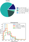 |
Fig. 3 Quality and homogeneity of the Level 0 data stored in the archive. Top panel: pie chart of the IBIS-A data divided for the median value of the quality image parameter q (in arcsec) during acquisition of Level 0 data (see Sect. 3.1 for details). Bottom panel: number of Level 0 datasets depending on their duration d and homogeneity of the quality image parameter q during observations. The homogeneity of the dataset is described by the standard deviation of the q values measured during the observing run. |
Overview of the Level 1.5 and Level 2 data available in IBIS-A.
3.2 Contextual and coordinated observations
The data stored at IBIS-A are characterized by the large volume of each target observation and the challenging analysis that is typical of any spectropolarimetric measurements. Nevertheless, the literature is rich in novel results derived from the analysis of data either belonging to or similar to those in IBIS-A. Almost all these studies, as well as the ones listed in Sect. 1, clearly show that combining spectropolarimetric measurements such as those in IBIS-A with data from other instruments greatly enhances the return of the scientific analysis of these observations by expanding the FOV and range of atmospheric heights that can be investigated. In this light, the IBIS-A archive offers its users links to observations complementary to the IBIS series available in the archive, such as those from co-temporal and near co-temporal high-resolution observations of the solar atmosphere available from the instruments on board the Hinode/SOT (Tsuneta et al. 2008) and IRIS (De Pontieu et al. 2014) satellites, and full-disk filtergrams from INAF solar telescopes (Ermolli et al. 2011; Romano et al. 2022).
Figure 4 shows examples of contextual data available in IBIS-A for the IBIS dataset obtained on 22 October 2014 observing the active region (AR) NOAA 12192. The contextual data include full-disk observations of the solar photosphere (not shown) and chromosphere at the Hα 6563 Å and Ca II K 3933 Å lines acquired by the INAF Catania and Rome/PSPT telescopes on the same day as the IBIS observations, and a magnification of the central region of AR NOAA 12192 from Hinode/SOT observations almost co-temporal with the IBIS measurements stored in IBIS-A. The latter pertain to the inner part of the AR during the occurrence of a X1.6 flare. It is worth noting that at present users are only provided with direct links to the Hinode/SOT and IRIS data complementary to those available for each series in IBIS-A, without any processing, for example to scale and target observations from the diverse instruments.
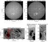 |
Fig. 4 Examples of contextual data available in IBIS-A. Full-disk observations of the solar chromosphere acquired on 22 October 2014 at the Hα (top left) and Ca II K (top right) lines by the INAF Catania and Rome/PSPT telescopes, respectively, and a zoom-in on the Hinode/SOT observation (Level 1) of the central region of NOAA AR 12192 (bottom left), also imaged by the IBIS data available in IBIS-A (bottom right). |
4 Data access
The IBIS-A data are stored on a RS24S3 SuperNAS server (96 TB, 64 GB Ram, 2 CPU Haswell 4C E5-2623V3 3G) at the INAF Osservatorio Astronomico di Roma6.
The metadata of the Level 0 files were incorporated into a MySQL database (DB) by using a Python application. The Python Django framework was used both to define the relational table schema using its object-relational internal mapping and to provide the web pages with simple query search interface.
The IBIS-A archive, so built, works on the server running Python 2.7.6, with Django version 1.9.1 on a MySQL 5.5 server. It has recently been tested (to update the query service) on a test machine running Python 3.9.1, Django 3.2.9, and a MySQL 8.0 server.
The interface permits data to be searched according to various criteria: solar target, disk position, observational mode, data range. The criteria can be combined in order to refine searches. Based on the metadata stored on the IBIS-A DB, the data search dynamically generates a HTML page with information about the available data. The HTML tabular output is prepared using Django views for the search results and formatted in HTML using the internal Django template tools. The products of the data search also include movies and plots of the atmospheric seeing during observations, as basic information to allow users to assess the data quality. The movies for quick-look purposes were created by using the 2D plotting library Matplotlib (version 1.5.2).
Browsing IBIS-A does not require authentication, but users have to register and log in to be able to request and download IBIS-A data.
5 A glimpse at science with IBIS-A
A significant fraction of the observations stored in IBIS-A are still scientifically unexplored. Figure 5 displays examples of these data. They concern calibrated observations of flaring regions obtained at the photospheric Fe I 6173 Å line and at the chromospheric Hα 6563 Å line (the latter is shown in Fig. 5 panels A and B at two different wavelengths) and Ca II 8542 Å line (Fig. 5 panels C and D) on 10 October 2014, 14:25 UT and 13 May 2016, 15:00 UT, at disk positions μ = 0.47 and μ = 0.89, respectively. The observations of these flaring regions exceed 100 min each.
The atmosphere imaged in the wing of Ca II 8542 Å (Fig. 5 panel C) is typical of the middle photosphere, with a clear pattern of reversed granulation. Instead, the wing of Hα 6563 Å, and the core of both Hα 6563 Å and Ca II 8542 Å (Fig. 5 panels A, B, D) show various parts of the chromosphere, with the typical dazzling variety of features such as surges, bundles of arch filament systems, spicules, and localized and extended bright regions. Figure 6 shows science-ready data available in IBIS-A for the flaring region with pores shown in panels C and D of Fig. 5. On the left side of the FOV, the maps of CP derived from the photospheric Fe I 6173 Å and chromospheric Ca II 8542 Å data (Fig. 6 panels F and G, respectively), and the map of the field inclination obtained from the VFISV data inversion (Fig. 6 panel D) reveal magnetic field concentrations with opposite polarity with respect to that in the pores. At the same location, the chromospheric observations at the Ca II line core (Fig. 5 panel D) display a filament and a footpoint of the flaring region (see X = [0, 100], Y = [300, 400]). Magnetic signatures of these structures are also found in the chromospheric CP map from Ca II 8542 Å data (Fig. 6 panel G). The maps of the magnetic field strength derived from inversion of the photospheric Fe I 6173 Å data (Fig. 6 panels B, C, and A, respectively) show values up to 1.4 kG in the pores and field strength in the range of 0.4–0.6 kG in their surrounding area. There the maps of the photopsheric LP and Vlos from the Fe I 6173 Å data (Fig. 6 panels E and H, respectively) show horizontal magnetic fields and velocity fields with strong upflows.
Figure 7 gives examples of the Level 1, Level 1.5, and Level 2 data available in IBIS-A for the spectropolarimetric observations of a sunspot region shown in Fig. 1. That region was observed on 13 May 2016, 15:38 UT at disk position μ = 0.67. It is worth noting that both Figs. 6 and 7 show values of the field inclination derived from data inversion in quiet-Sun areas peaked around 90°. As reported by Borrero & Kobel (2011), these values result from the inversion of LP measurements characterized by a signal-to-noise ratio lower than 4.5. However, a more accurate estimate of the magnetic field inclination in quiet Sun regions is beyond the scope of the present work, which aims to provide quick-look science-ready data to IBIS-A users.
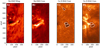 |
Fig. 5 Examples of Level 1 data of chromospheric flaring regions available in IBIS-A. The data were acquired along the Hα 6563 Å line, in the wing (panel A) and core (panel B) of the line, on 10 October 2014, 14:20 UT at disk position μ = 0.43, and along the Ca II 8542 Å line, in the far wing (panel C) and line core (panel D), on 13 May 2016, 15:00 UT, at disk position μ = 0.9. The white lines in the rightmost panels show contours of the magnetic pore regions corresponding to Ic(x, y) = 0.8 × Ic (quiet), where Ic(x, y) and Ic (quiet) are values of the line continuum intensity at the given position (x, y) and in the quiet region. |
6 Summary and conclusions
This paper presents the IBIS-A archive, which currently includes 30TB of data taken with the Interferometric BIdimensional Spectropolarimeter (IBIS) during 28 observing campaigns carried out from 2008 to 2019 over 159 days. This presentation of the archive is meant to facilitate and foster the scientific usage of the IBIS-A data with examples of the data quality and their application in recent and undergoing studies relevant to solar processes and space weather science.
Since the implementation of IBIS-A in 2016, the raw data available in the archive have increased, as has the fraction of calibrated measurements. In addition, links have been added pointing to complementary data of the solar atmosphere available from coordinated measurements performed with the instruments on board the Hinode and IRIS satellites, and the full-disk red continuum, Ca II K, and Hα observations of the photosphere and chromosphere from the INAF synoptic solar telescopes.
Furthermore, the archive has been populated with higher level products from inversion of the calibrated data. Multidimensional arrays with maps of circular, linear, and net circular polarization, and los velocity patterns from calibrated photospheric Fe 16173 Å and chromospheric Ca II 8542 Å series are also offered to registered users. In addition, more than 80% of the calibrated Fe I 6173 Å photospheric series have already been inverted with the VFISV code to offer a quick-look view of the magnetic and velocity fields in the archived targets. A further milestone will be reached from the inversion of the remaining photospheric data and of the chromospheric series with the new NLTE DeSIRe code (Ruiz Cobo et al. 2022). The IBIS-A team will also incorporate more data in the archive when they become available.
The IBIS-A data include metadata for proper interpretation and archiving of the observations available in the archive. At present, the keywords employed in the header of FITS Level 1.5 and Level 2 data are partly compliant7 with the recently formulated SOLARNET recommendations. The complete standardization of the metadata information provided by the IBIS-A data planned in the near future will facilitate their usage by users with limited knowledge of the spectropolarimetric observations. In addition, it will allow easy inclusion of IBIS-A data in future Solar Virtual Observatories.
IBIS-A represents a unique resource for investigating the plasma processes in the solar atmosphere and the solar origin of Space Weather events. In addition, it represents the prototype of the archive that will host the data acquired with the updated version of the IBIS instrument, named IBIS 2.0, which is under development for installation at the Osservatorio del Roque de Los Muchachos in the Canary Islands.
Browsing IBIS-A does not require authentication, but users have to register and log in to be able to request and download data. The IBIS-A team is open for technical support and help with the data analysis to foster the use of data stored in the archive in new science projects. In this respect, we note that IBIS-A is currently maintained by the H2020 SOLARNET High-resolution Solar Physics Network project, which aims at integrating the major European infrastructures in the field of high-resolution solar physics. Therefore, any publication that uses data contained in IBIS-A should acknowledge the above support by reporting “This study makes use of data collected in the IBIS-A archive, which has received funding from the European Union’s Horizon 2020 research and innovation programme under Grant Agreements No. 824135 (SOLARNET).”
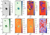 |
Fig. 6 Examples of Level 1, Level 1.5, and Level 2 data available in IBIS-A for the flaring region with magnetic pores shown in Fig. 5. The observations were taken on 13 May 2016 at 15:00 UT. The top panels show Level 1 (panel A) and Level 2 (panels B–D) data, while the bottom panels show Level 1.5 (panels E–H) data. Top panels, from left to right: maps of the intensity measured on the FOV at the Fe 16173 Å line continuum and of the magnetic field strength, azimuth, and inclination angles derived from the VFISV inversion of the Fe I 6173 Å line data. Bottom panels, from left to right: maps of the linear and circular polarization estimated from the photospheric Fe I 6173 Å line data, circular polarization from the chromospheric Ca II 8542 Å observations, and los velocity field at photopheric heights from Fe I 6173 Å measurements (see Fig. 5 for more details). |
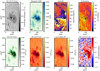 |
Fig. 7 Examples of Level 1, Level 1.5, and Level 2 data available in IBIS-A for the sunspot region observed on 13 May 2016, 13:38 UT at disk position μ = 0.68 shown in Fig. 1. The top panels show Level 1 (panel A) and Level 2 (panels B–D) data, while the bottom panels show Level 1.5 (panels E–H) data (see Figs. 5 and 6 for more details). |
Acknowledgements
The authors thank Doug Gilliam and Mike Bradford for acquisition of IBIS data throughout the years. They also thank Juan Manuel Borrero and Han Uitenbroek for their work on IBIS data. The authors are grateful to the referee for carefully reading of the paper and for her/his comments. This research has received funding from the European Union’s FP7 Capacities program under grant agreement No 312495 (SOLARNET) and from the European Union’s Horizon 2020 Research and Innovation program under grant agreements No 824135 (SOLARNET) and No 739500 (PRE-EST). This work was also supported by the Italian MIUR-PRIN grant 2017 “Circumterrestrial Environment: Impact of Sun–Earth Interaction” and by the INAF Istituto Nazionale di Astrofísica. The Level 2 data available in IBIS-A were obtained from access to servers of the Italian CINECA and INAF. IBIS has been designed and constructed by the INAF Osservatorio Astrofísico di Arcetri with contributions from the Universitá di Firenze, the Universitá di Roma Tor Vergata, and upgraded with further contributions from National Solar Observatory (NSO) and Queens University Belfast. IBIS was operated with support of the NSO. The NSO is operated by the Association of Universities for Research in Astronomy, Inc., under cooperative agreement with the National Science Foundation. This research made use of NASA’s Astrophysics Data System.
Appendix A Data summary and metadata information
Table A.1 summarizes the information on the Level 1 data available in IBIS-A. These data consist of the observations processed for instrumental calibrations and restored for residual image degradation by seeing using the MOMFBD method. Table A.2 summarizes information on the Level 2 data available in IBIS-A. These data consist of the observations processed for data inversion using the VFISV code. More details on the Level 1 and Level 2 data can be found in Sect. 2.3.
Figures A.1 and A.2 show examples of metadata information provided in the keywords of the primary and extended headers of FITS files of the Level 0 data available in IBIS-A. Figure A.3 gives an example of the fields with information stored in the variable info_nb relevant to Level 1 data. Figure A.4 and A.5 show examples of the metadata information provided in the keywords of the primary and extended headers of FITS files of the Level 1.5 data, respectively. figure A.6 displays the same information for Level 2 data. See Sect. 3.1 for more details.
Overview of the Level 1 data available in IBIS-A.
 |
Fig. A.1 Example of metadata information stored in the FITS primary header of the Level 0 data available in IBIS-A for the observations taken on 28 May 2012 at 13:38:43 UT. |
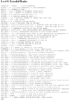 |
Fig. A.2 Example of metadata information stored in the FITS extended header of the Level 0 data available in IBIS-A for the observations taken on 28 May 2012 at 13:38:43 UT. |
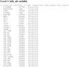 |
Fig. A.3 Example of several fields with information stored in the info_nb variable, which is relevant to the Level 1 data derived from the spectropolarimetric observations taken at the Fe I 617.3 nm line on 13 May 2016 at 13:38:48 UT. |
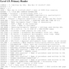 |
Fig. A.4 Example of metadata information stored in the FITS primary header of the Level 1.5 data available in IBIS-A for the observations taken on 13 May 2016 at 13:38:48 UT. |
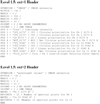 |
Fig. A.5 Example of metadata information stored in the FITS extended header of the Level 1.5 data available in IBIS-A for the observations taken on 13 May 2016 at 13:38:48 UT. |
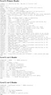 |
Fig. A.6 Example of metadata information stored in the FITS header of the Level 2 data available in IBIS-A for the observations taken on 13 May 2016 at 13:38 UT. |
Overview of the Level 2 data available in IBIS-A.
References
- Abbasvand, V., Sobotka, M., Heinzel, P., et al. 2020, ApJ, 890, 22 [Google Scholar]
- Baker, D., Stangalini, M., Valori, G., et al. 2021, ApJ, 907, 16 [Google Scholar]
- Bellot Rubio, L., & Orozco Suárez, D. 2019, Liv. Rev. Sol. Phys., 16, 1 [Google Scholar]
- Blandford, R., Meier, D., & Readhead, A. 2019, ARA&A, 57, 467 [NASA ADS] [CrossRef] [Google Scholar]
- Borrero, J. M., & Kobel, P. 2011, A&A, 527, A29 [NASA ADS] [CrossRef] [EDP Sciences] [Google Scholar]
- Borrero, J. M., Tomczyk, S., Kubo, M., et al. 2011, Sol. Phys., 273, 267 [Google Scholar]
- Borrero, J. M., Jafarzadeh, S., Schüssler, M., & Solanki, S. K. 2017, Space Sci. Rev., 210, 275 [Google Scholar]
- Brosius, J. W., Daw, A. N., & Rabin, D. M. 2014, ApJ, 790, 112 [NASA ADS] [CrossRef] [Google Scholar]
- Cao, W., Gorceix, N., Coulter, R., et al. 2010, SPIE Conf. Ser., 7735, 77355V [Google Scholar]
- Capparelli, V., Zuccarello, F., Romano, P., et al. 2017, ApJ, 850, 36 [NASA ADS] [CrossRef] [Google Scholar]
- Cauzzi, G., Reardon, K. P., Uitenbroek, H., et al. 2008, A&A, 480, 515 [NASA ADS] [CrossRef] [EDP Sciences] [Google Scholar]
- Cauzzi, G., Reardon, K., Rutten, R. J., Tritschler, A., & Uitenbroek, H. 2009, A&A, 503, 577 [NASA ADS] [CrossRef] [EDP Sciences] [Google Scholar]
- Cavallini, F. 2006, Sol. Phys., 236, 415 [NASA ADS] [CrossRef] [Google Scholar]
- Cheung, M. C. M., & Isobe, H. 2014, Liv. Rev. Sol. Phys., 11, 3 [Google Scholar]
- Collados, M., Bettonvil, F., Cavaller, L., et al. 2013, Mem. Soc. Astron. Italiana, 84, 379 [NASA ADS] [Google Scholar]
- Criscuoli, S., & Tritschler, A. 2014, IBIS Data Reduction Notes, Tech. Rep. NS05, National Solar Observatory, Sacramento Peak [Google Scholar]
- Criscuoli, S., Del Moro, D., Giannattasio, F., et al. 2012, A&A, 546, A26 [NASA ADS] [CrossRef] [EDP Sciences] [Google Scholar]
- Criscuoli, S., Ermolli, I., Uitenbroek, H., & Giorgi, F. 2013, ApJ, 763, 144 [NASA ADS] [CrossRef] [Google Scholar]
- Del Moro, D., Giordano, S., & Berrilli, F. 2007, A&A, 472, 599 [NASA ADS] [CrossRef] [EDP Sciences] [Google Scholar]
- del Toro Iniesta, J.C., & Ruiz Cobo, B. 2016, Liv. Rev. Sol. Phys., 13, 4 [NASA ADS] [CrossRef] [Google Scholar]
- De Pontieu, B., Title, A. M., Lemen, J. R., et al. 2014, Sol. Phys., 289, 2733 [Google Scholar]
- Ermolli, I., Criscuoli, S., & Giorgi, F. 2011, Contrib. Astron. Observ. Skalnate Pleso, 41, 73 [NASA ADS] [Google Scholar]
- Ermolli, I., Cristaldi, A., Giorgi, F., et al. 2017, A&A, 600, A102 [NASA ADS] [CrossRef] [EDP Sciences] [Google Scholar]
- Ermolli, I., Cirami, R., Calderone, G., et al. 2020, SPIE Conf. Ser., 11447, 114470Z [Google Scholar]
- Giordano, S., Berrilli, F., Del Moro, D., & Penza, V. 2008, A&A, 489, 747 [NASA ADS] [CrossRef] [EDP Sciences] [Google Scholar]
- Harris, C. R., Millman, K. J., van der Walt, S.J., et al. 2020, Nature, 585, 357 [NASA ADS] [CrossRef] [Google Scholar]
- Haugan, S. V. H., & Fredvik, T. 2015, Document on Standards for Data Archiving and VO, Deliverable D20.4, SOLARNET (EC 7th FP grant 312495, Tech. Rep. D20.4, Institute of Theoretical Astrophysics, University of Oslo [Google Scholar]
- Haugan, S. V. H., & Fredvik, T. 2020, ArXiv e-prints, [arXiv:2011.12139] [Google Scholar]
- Houston, S. J., Jess, D. B., Keppens, R., et al. 2020, ApJ, 892, 49 [NASA ADS] [CrossRef] [Google Scholar]
- Hunter, J. D. 2007, Comput. Sci. Eng., 9, 90 [NASA ADS] [CrossRef] [Google Scholar]
- Jaeggli, S. A., Lin, H., & Uitenbroek, H. 2012, ApJ, 745, 133 [NASA ADS] [CrossRef] [Google Scholar]
- Jess, D. B., Mathioudakis, M., Christian, D. J., et al. 2010, Sol. Phys., 261, 363 [NASA ADS] [CrossRef] [Google Scholar]
- Jess, D. B., Morton, R. J., Verth, G., et al. 2015, Space Sci. Rev., 190, 103 [Google Scholar]
- Judge, P. G., Tritschler, A., Uitenbroek, H., et al. 2010, ApJ, 710, 1486 [NASA ADS] [CrossRef] [Google Scholar]
- Kilpua, E., Koskinen, H. E. J., & Pulkkinen, T. I. 2017, Liv. Rev. Sol. Phys., 14, 5 [Google Scholar]
- Kobayashi, K., Cirtain, J., Winebarger, A. R., et al. 2014, Sol. Phys., 289, 4393 [Google Scholar]
- Kowalski, A. F., Cauzzi, G., & Fletcher, L. 2015, ApJ, 798, 107 [NASA ADS] [CrossRef] [Google Scholar]
- Lemen, J. R., Title, A. M., Akin, D. J., et al. 2012, Sol. Phys., 275, 17 [Google Scholar]
- Lipartito, I., Judge, P. G., Reardon, K., & Cauzzi, G. 2014, ApJ, 785, 109 [NASA ADS] [CrossRef] [Google Scholar]
- Löfdahl, M. 2012, IAU Special Session, 6, E3.05 [Google Scholar]
- Löfdahl, M. 2016, in ASP Conf. Ser., 504, >Coimbra Solar Physics Meeting: Ground-based Solar Observations in the Space Instrumentation Era, eds. I. Dorotovic, C.E. Fischer, & M. Temmer, 111 [Google Scholar]
- Löfdahl, M. G., Hillberg, T., de la Cruz Rodríguez, J., et al. 2021, A&A, 653, A68 [Google Scholar]
- Martínez Pillet V., Del Toro Iniesta, J.C., Álvarez-Herrero, A., et al. 2011, Sol. Phys., 268, 57 [CrossRef] [Google Scholar]
- Molnar, M. E., Reardon, K. P., Chai, Y., et al. 2019, ApJ, 881, 99 [Google Scholar]
- Murabito, M., Romano, P., Guglielmino, S. L., Zuccarello, F., & Solanki, S. K. 2016, ApJ, 825, 75 [NASA ADS] [CrossRef] [Google Scholar]
- Murabito, M., Romano, P., Guglielmino, S. L., & Zuccarello, F. 2017, ApJ, 834, 76 [NASA ADS] [CrossRef] [Google Scholar]
- Murabito, M., Ermolli, I., Giorgi, F., et al. 2019, ApJ, 873, 126 [NASA ADS] [CrossRef] [Google Scholar]
- Murabito, M., Guglielmino, S. L., Ermolli, I., Stangalini, M., & Giorgi, F. 2020a, ApJ, 890, 96 [NASA ADS] [CrossRef] [Google Scholar]
- Murabito, M., Shetye, J., Stangalini, M., et al. 2020b, A&A, 639, A59 [EDP Sciences] [Google Scholar]
- Narukage, N., McKenzie, D. E., Ishikawa, R., et al. 2016, SPIE Conf. Ser., 9905, 990508 [NASA ADS] [Google Scholar]
- Padoan, P., & Nordlund, Å. 2011, ApJ, 730, 40 [Google Scholar]
- Rast, M. P., Bello González, N., Bellot Rubio, L., et al. 2021, Sol. Phys., 296, 70 [NASA ADS] [CrossRef] [Google Scholar]
- Reardon, K. P., & Cavallini, F. 2008, A&A, 481, 897 [NASA ADS] [CrossRef] [EDP Sciences] [Google Scholar]
- Reardon, K. P., Uitenbroek, H., & Cauzzi, G. 2009, A&A, 500, 1239 [NASA ADS] [CrossRef] [EDP Sciences] [Google Scholar]
- Rempel, M., & Schlichenmaier, R. 2011, Liv. Rev. Sol. Phys., 8, 3 [Google Scholar]
- Righini, A., Cavallini, F., & Reardon, K. P. 2010, A&A, 515, A85 [NASA ADS] [CrossRef] [EDP Sciences] [Google Scholar]
- Rimmele, T.R., Warner, M., Keil, S.L., et al. 2020, Sol. Phys., 295, 172 [NASA ADS] [CrossRef] [Google Scholar]
- Romano, P., Berrilli, F., Criscuoli, S., et al. 2012, Sol. Phys., 280, 407 [CrossRef] [Google Scholar]
- Romano, P., Frasca, D., Guglielmino, S. L., et al. 2013, ApJ, 771, L3 [NASA ADS] [CrossRef] [Google Scholar]
- Romano, P., Zuccarello, F. P., Guglielmino, S. L., & Zuccarello, F. 2014, ApJ, 794, 118 [NASA ADS] [CrossRef] [Google Scholar]
- Romano, P., Falco, M., Guglielmino, S. L., & Murabito, M. 2017, ApJ, 837, 173 [NASA ADS] [CrossRef] [Google Scholar]
- Romano, P., Murabito, M., Guglielmino, S. L., Zuccarello, F., & Falco, M. 2020, ApJ, 899, 129 [NASA ADS] [CrossRef] [Google Scholar]
- Romano, P., Guglielmino, S.L., Costa, P., et al. 2022, Sol. Phys., 297, 7 [NASA ADS] [CrossRef] [Google Scholar]
- Ruiz Cobo, B., Quintero Noda, C., Gafeira, R., et al. 2022, A&A, 660, A37 [NASA ADS] [CrossRef] [EDP Sciences] [Google Scholar]
- Scharmer, G. B., Bjelksjo, K., Korhonen, T. K., Lindberg, B., & Petterson, B. 2003, SPIE Conf. Ser., 4853, 341 [NASA ADS] [Google Scholar]
- Scharmer, G. B., Narayan, G., Hillberg, T., et al. 2008, ApJ, 689, L69 [Google Scholar]
- Scharmer, G. B., Löfdahl, M. G., Sliepen, G., & de la Cruz Rodríguez, J. 2019, A&A, 626, A55 [NASA ADS] [CrossRef] [EDP Sciences] [Google Scholar]
- Scherrer, P. H., Bogart, R. S., Bush, R. I., et al. 1995, Sol. Phys., 162, 129 [Google Scholar]
- Scherrer, P. H., Schou, J., Bush, R. I., et al. 2012, Sol. Phys., 275, 207 [Google Scholar]
- Schilliro, F., & Romano, P. 2021, MNRAS, 503, 2676 [NASA ADS] [CrossRef] [Google Scholar]
- Schlichenmaier, R., & Schmidt, W. 2000, A&A, 358, 1122 [NASA ADS] [Google Scholar]
- Schlichenmaier, R., Bellot Rubio, L. R., Collados, M., et al. 2019, ArXiv e-prints, [arXiv:1912.08650] [Google Scholar]
- Schmelz, J. T. 2003, Advances in Space Research, 32, 895 [NASA ADS] [CrossRef] [Google Scholar]
- Seykora, E. J. 1993, Sol. Phys., 145, 389 [NASA ADS] [CrossRef] [Google Scholar]
- Sobotka, M., Del Moro, D., Jurčák, J., & Berrilli, F. 2012, A&A, 537, A85 [NASA ADS] [CrossRef] [EDP Sciences] [Google Scholar]
- Sobotka, M., Švanda, M., Jurčák, J., et al. 2013, A&A, 560, A84 [EDP Sciences] [Google Scholar]
- Sobotka, M., Heinzel, P., Švanda, M., et al. 2016, ApJ, 826, 49 [Google Scholar]
- Solanki, S. K., & Montavon, C. A. P. 1993, A&A, 275, 283 [NASA ADS] [Google Scholar]
- Stangalini, M., Del Moro, D., Berrilli, F., & Jefferies, S. M. 2011, A&A, 534, A65 [NASA ADS] [CrossRef] [EDP Sciences] [Google Scholar]
- Stangalini, M., Giannattasio, F., Del Moro, D., & Berrilli, F. 2012, A&A, 539, L4 [NASA ADS] [CrossRef] [EDP Sciences] [Google Scholar]
- Stangalini, M., Berrilli, F., & Consolini, G. 2013, A&A, 559, A88 [NASA ADS] [CrossRef] [EDP Sciences] [Google Scholar]
- Stangalini, M., Jafarzadeh, S., Ermolli, I., et al. 2018, ApJ, 869, 110 [Google Scholar]
- Stangalini, M., Baker, D., Valori, G., et al. 2021a, Philos. Trans. R. Soc. Lond. A, 379, 20200216 [Google Scholar]
- Stangalini, M., Erdélyi, R., Boocock, C., et al. 2021b, Nat. Astron., 5, 691 [NASA ADS] [CrossRef] [Google Scholar]
- Stangalini, M., Jess, D. B., Verth, G., et al. 2021c, A&A, 649, A169 [NASA ADS] [CrossRef] [EDP Sciences] [Google Scholar]
- Stangalini, M., Verth, G., Fedun, V., et al. 2022, Nat. Astron., 13, 479 [Google Scholar]
- Stein, R. F. 2012, Liv. Rev. Sol. Phys., 9, 4 [Google Scholar]
- Straus, T., Fleck, B., Jefferies, S. M., et al. 2008, ApJ, 681, L125 [Google Scholar]
- Temmer, M. 2021, Liv. Rev. Sol. Phys., 18, 4 [NASA ADS] [CrossRef] [Google Scholar]
- Tritschler, A., Uitenbroek, H., & Reardon, K. 2008, ApJ, 686, L45 [Google Scholar]
- Tsuneta, S., Ichimoto, K., Katsukawa, Y., et al. 2008, Sol. Phys., 249, 167 [Google Scholar]
- van Driel-Gesztelyi, L., & Green, L.M. 2015, Liv. Rev. Sol. Phys., 12, 1 [CrossRef] [Google Scholar]
- van Noort M., Rouppe van der Voort, L., & Löfdahl, M.G. 2005, Sol. Phys., 228, 191 [NASA ADS] [CrossRef] [Google Scholar]
- Vecchio, A., Cauzzi, G., Reardon, K. P., Janssen, K., & Rimmele, T. 2007, A&A, 461, L1 [CrossRef] [EDP Sciences] [Google Scholar]
- Vecchio, A., Cauzzi, G., & Reardon, K. P. 2009, A&A, 494, 269 [NASA ADS] [CrossRef] [EDP Sciences] [Google Scholar]
- Viavattene, G., Consolini, G., Giovannelli, L., et al. 2020, Entropy, 22, 716 [NASA ADS] [CrossRef] [Google Scholar]
- Viavattene, G., Murabito, M., Guglielmino, S. L., et al. 2021, Entropy, 23, 413 [NASA ADS] [CrossRef] [Google Scholar]
- Virtanen, P., Gommers, R., Oliphant, T. E., et al. 2020, Nat. Methods, 17, 261 [Google Scholar]
- Vissers, G., & Rouppe van der Voort, L. 2012, ApJ, 750, 22 [Google Scholar]
- Viticchié, B., Del Moro, D., Berrilli, F., Bellot Rubio, L., & Tritschler, A. 2009, ApJ, 700, L145 [CrossRef] [Google Scholar]
- Viticchié, B., Del Moro, D., Criscuoli, S., & Berrilli, F. 2010, ApJ, 723, 787 [CrossRef] [Google Scholar]
- Vourlidas, A., Beltran, S. T., Chintzoglou, G., et al. 2016, J. Astron. Instrum., 5, 1640003 [NASA ADS] [CrossRef] [Google Scholar]
- Wedemeyer, S., Szydlarski, M., Jafarzadeh, S., et al. 2020, A&A, 635, A71 [NASA ADS] [CrossRef] [EDP Sciences] [Google Scholar]
- Wiegelmann, T., & Sakurai, T. 2021, Liv. Rev. Sol. Phys., 18, 1 [NASA ADS] [CrossRef] [Google Scholar]
- Zuccarello, F., Romano, P., Guglielmino, S. L., et al. 2009, A&A, 500, L5 [NASA ADS] [CrossRef] [EDP Sciences] [Google Scholar]
Interactive Data Language, Harris Geospatial Solutions, Inc.
Currently available only for spectropolarimetric series.
At present, FITS Standard Version 3 using CFITSIO Version 3.47.
From both of the above-mentioned calculations applied.
The IBIS-A data can be accessed at http://ibis.oa-roma.inaf.it/IBISA/
Following the definition in relevant documents.
All Tables
All Figures
|
Fig. 1 Examples of IBIS data acquired (from left to right) in standard spectroscopic and spectropolarimetric modes at the Fe I 6173 Å line with circular (1000 × 1000 pixels2) and rectangular (350 × 800 pixels2) FOV on 25 October 2014, 15:32 UT and 13 May 2016, 13:38 UT at disk positions μ = 0.85 and μ = 0.68, respectively. The spectroscopic and spectropolarimetric Stokes I observations were taken in the line continuum, while the spectropolarimetric Stokes Q and Stokes U and V data were acquired in the line core and line blue wing, respectively. Shown here are the Level 1 data derived from the instrumental calibrations and MOMFBD restoration (see Sects. 2.2 and 3.1 for more details). |
| In the text | |
|
Fig. 2 Level 0 data stored in the archive. Shown are pie charts of the fraction (in %) of panel a) the spectroscopic and spectropolarimetric data available in IBIS-A, panel b) the spectral lines (in Å) acquired during the observations, panel c) the duration (in minutes) of the observational sequences, and panel d) the μ disk position of the FOV (μ = cosθ where θ is the heliocentric angle). |
| In the text | |
|
Fig. 3 Quality and homogeneity of the Level 0 data stored in the archive. Top panel: pie chart of the IBIS-A data divided for the median value of the quality image parameter q (in arcsec) during acquisition of Level 0 data (see Sect. 3.1 for details). Bottom panel: number of Level 0 datasets depending on their duration d and homogeneity of the quality image parameter q during observations. The homogeneity of the dataset is described by the standard deviation of the q values measured during the observing run. |
| In the text | |
|
Fig. 4 Examples of contextual data available in IBIS-A. Full-disk observations of the solar chromosphere acquired on 22 October 2014 at the Hα (top left) and Ca II K (top right) lines by the INAF Catania and Rome/PSPT telescopes, respectively, and a zoom-in on the Hinode/SOT observation (Level 1) of the central region of NOAA AR 12192 (bottom left), also imaged by the IBIS data available in IBIS-A (bottom right). |
| In the text | |
|
Fig. 5 Examples of Level 1 data of chromospheric flaring regions available in IBIS-A. The data were acquired along the Hα 6563 Å line, in the wing (panel A) and core (panel B) of the line, on 10 October 2014, 14:20 UT at disk position μ = 0.43, and along the Ca II 8542 Å line, in the far wing (panel C) and line core (panel D), on 13 May 2016, 15:00 UT, at disk position μ = 0.9. The white lines in the rightmost panels show contours of the magnetic pore regions corresponding to Ic(x, y) = 0.8 × Ic (quiet), where Ic(x, y) and Ic (quiet) are values of the line continuum intensity at the given position (x, y) and in the quiet region. |
| In the text | |
|
Fig. 6 Examples of Level 1, Level 1.5, and Level 2 data available in IBIS-A for the flaring region with magnetic pores shown in Fig. 5. The observations were taken on 13 May 2016 at 15:00 UT. The top panels show Level 1 (panel A) and Level 2 (panels B–D) data, while the bottom panels show Level 1.5 (panels E–H) data. Top panels, from left to right: maps of the intensity measured on the FOV at the Fe 16173 Å line continuum and of the magnetic field strength, azimuth, and inclination angles derived from the VFISV inversion of the Fe I 6173 Å line data. Bottom panels, from left to right: maps of the linear and circular polarization estimated from the photospheric Fe I 6173 Å line data, circular polarization from the chromospheric Ca II 8542 Å observations, and los velocity field at photopheric heights from Fe I 6173 Å measurements (see Fig. 5 for more details). |
| In the text | |
|
Fig. 7 Examples of Level 1, Level 1.5, and Level 2 data available in IBIS-A for the sunspot region observed on 13 May 2016, 13:38 UT at disk position μ = 0.68 shown in Fig. 1. The top panels show Level 1 (panel A) and Level 2 (panels B–D) data, while the bottom panels show Level 1.5 (panels E–H) data (see Figs. 5 and 6 for more details). |
| In the text | |
|
Fig. A.1 Example of metadata information stored in the FITS primary header of the Level 0 data available in IBIS-A for the observations taken on 28 May 2012 at 13:38:43 UT. |
| In the text | |
|
Fig. A.2 Example of metadata information stored in the FITS extended header of the Level 0 data available in IBIS-A for the observations taken on 28 May 2012 at 13:38:43 UT. |
| In the text | |
|
Fig. A.3 Example of several fields with information stored in the info_nb variable, which is relevant to the Level 1 data derived from the spectropolarimetric observations taken at the Fe I 617.3 nm line on 13 May 2016 at 13:38:48 UT. |
| In the text | |
|
Fig. A.4 Example of metadata information stored in the FITS primary header of the Level 1.5 data available in IBIS-A for the observations taken on 13 May 2016 at 13:38:48 UT. |
| In the text | |
|
Fig. A.5 Example of metadata information stored in the FITS extended header of the Level 1.5 data available in IBIS-A for the observations taken on 13 May 2016 at 13:38:48 UT. |
| In the text | |
|
Fig. A.6 Example of metadata information stored in the FITS header of the Level 2 data available in IBIS-A for the observations taken on 13 May 2016 at 13:38 UT. |
| In the text | |
Current usage metrics show cumulative count of Article Views (full-text article views including HTML views, PDF and ePub downloads, according to the available data) and Abstracts Views on Vision4Press platform.
Data correspond to usage on the plateform after 2015. The current usage metrics is available 48-96 hours after online publication and is updated daily on week days.
Initial download of the metrics may take a while.