| Issue |
A&A
Volume 661, May 2022
|
|
|---|---|---|
| Article Number | A109 | |
| Number of page(s) | 9 | |
| Section | Planets and planetary systems | |
| DOI | https://doi.org/10.1051/0004-6361/202142683 | |
| Published online | 24 May 2022 | |
A quantitative assessment of the VO line list: Inaccuracies hamper high-resolution VO detections in exoplanet atmospheres
1
Leiden Observatory, Leiden University,
Postbus 9513,
2300
RA Leiden,
The Netherlands
e-mail: This email address is being protected from spambots. You need JavaScript enabled to view it.
2
Astrophysics Research Centre, School of Mathematics and Physics, Queen’s University Belfast,
Belfast
BT7 1NN,
UK
3
Centre for Exoplanet Science, University of St Andrews,
North Haugh,
St Andrews,
UK
4
Stellar Astrophysics Centre, Deparment of Physics and Astronomy, Aarhus University,
Ny Munkegade 120,
8000
Aarhus C,
Denmark
Received:
17
November
2021
Accepted:
20
February
2022
Abstract
Context. Metal hydrides and oxides are important species in hot-Jupiters since they can affect their energy budgets and the thermal structure of their atmospheres. One such species is vanadium-oxide (VO), which is prominent in stellar M-dwarf spectra. Evidence for VO has been found in the low-resolution transmission spectrum of WASP-121b, but this has not been confirmed at high resolution. It has been suggested that this is due to inaccuracies in its line list.
Aims. In this paper, we quantitatively evaluate the VO line list and assess whether inaccuracies are indeed the reason for the non-detections at high resolution in WASP-121b. Furthermore, we investigate whether the detectability can be improved by selecting only those lines associated with the most accurate quantum transitions.
Methods. A cross-correlation analysis was applied to archival High Accuracy Radial velocity Planet Searcher and CARMENES spectra of several M-dwarfs. VO cross-correlation signals from the spectra were compared with those in which synthetic VO models were injected, providing an estimate of the ratio between the potential strength (in case of a perfect model) and the observed strength of the signal. This was repeated for the reduced model covering the most accurate quantum transitions. The findings were subsequently fed into injection and recovery tests of VO in a Ultraviolet and Visual Echelle Spectrograph transmission spectrum of WASP-121b.
Results. We find that inaccuracies cause cross-correlation signals from VO in M-dwarf spectra to be suppressed by about a factor 2.1 and 1.1 for the complete and reduced line lists, respectively, corresponding to a reduced observing efficiency of a factor 4.3 and 1.2. The reduced line list outperforms the complete line list in recovering the actual VO signal in the M-dwarf spectra by about a factor of 1.8. Neither line list results in a VO detection in WASP-121b. Injection tests show that with the reduced efficiency of the line lists, the potential signal as seen at low resolution is not detectable in these data.
Key words: molecular data / opacity / stars: low-mass / planets and satellites: atmospheres / techniques: spectroscopic / planets and satellites: individual: WASP-121b
© ESO 2022
1 Introduction
Ultra-hot Jupiters (UHJs) are a class of gas giant exoplanets that orbit their host stars at extremely close distances and thus they are highly irradiated. Their equilibrium temperatures exceed Teq ≳ 2200 K, akin to low-mass stars (Lothringer & Barman 2019). One of the defining features of UHJs is the presence of a thermal inversion, caused by spectroscopically active species absorbing stellar radiation in the upper atmosphere. In this way, a thermal inversion affects a planet’s energy budget and the redistribution of absorbed stellar energy from day to nightside. Hubeny et al. (2003) and Fortney et al. (2008) suggested that UHJ atmospheres are hot enough to contain gaseous titanium oxide (TiO) and vanadium oxide (VO), as in low-mass stars. These metal oxides could possibly be responsible for the inversions strongly absorbing incoming UV and optical radiation at high altitudes and heating up the upper atmosphere.
In the case of UHJ WASP-121b, the presence of a thermal inversion has been observed using emission features in secondary eclipse Hubble Space Telescope (HST) spectra (Evans et al. 2017; Mikal-Evans et al. 2019, 2020), which is in line with the inefficient heat transport inferred from Transiting Exoplanet Survey Satellite (TESS) phase curve photometry (Daylan et al. 2021; Bourrier et al. 2020). Low-resolution spectroscopy has provided tentative evidence for VO in WASP-121b’s atmosphere (Evans et al. 2016, 2018; Mikal-Evans et al. 2019). High-resolution Doppler-resolved spectroscopy (Snellen et al. 2010; Brogi et al. 2012; Birkby et al. 2013) has been used in an effort to confirm the low-resolution VO detection. However, Hoeijmakers et al. (2020) analysed transmission spectra observed by the High Accuracy Radial velocity Planet Searcher (HARPS) to report a non-detection of VO. Furthermore, Merritt et al. (2020) present a non-detection using transmission spectra observed with the Ultraviolet and Visual Echelle Spectrograph (UVES), but both Merritt et al. (2020) and Hoeijmakers et al. (2020) stress that their VO non-detections are inconclusive as a consequence of the inaccuracies of the state-of-the-art ExoMol (Tennyson et al. 2020) VO line list (McKemmish et al. 2016). Indeed, Hoeijmakers et al. (2020) argue that their detection of V I implies the presence of VO as their equilibrium chemistry calculations show that a significant amount of vanadium should exist as gaseous VO.
In this paper, we present a quantitative assessment of the ExoMol VO line list to evaluate the discrepancy between the low-resolution evidence and the high-resolution non-detections of this molecule in the atmosphere of exoplanet WASP-121b. The line list’s cross-correlation performance is studied using highresolution spectra of M-dwarf stars in Sect. 2. In Sect. 3, the results of the line-list assessment are used to interpret the analysis of UVES transmission spectra of WASP-121b. Section 4 discusses the overall results and summarises the conclusions.
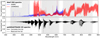 |
Fig. 1 Comparison between the observed M-dwarf spectra and the petitRADTRANS VO model spectra. Top panel: HARPS and CARMENES spectra of Wolf 359 in blue and red, respectively. Bottom panel: normalised VO model spectra using all quantum transitions in black and using the specific transitions described in Sect. 2.4 in grey. The grey vertical bands in both panels show the wavelength ranges of the UVES spectral orders. |
2 VO line-list assessment
The most recent and accurate VO line list was constructed by the ExoMol group (McKemmish et al. 2016) and it is available from the ExoMol library1. The line list consists of approximately 640 000 energy levels between which more than 277 million transitions are transcribed. The energy levels are determined using quantum chemistry calculations and then adjusted based on experimental data. The limited availability of experimental data results in poorly constrained energy levels, which subsequently translate into large wavelength uncertainties of spectral lines. As a result, model spectra made with the ExoMol line list are not an exact representation of the actual VO opacity at high resolution. The presented analysis uses the ExoMol VO line list with version number 20160726, where additional experimental data were used to further refine the A4Π, B4Π, and C4Σ− states from the initial publication (Laura McKemmish, priv. comm.). There is a Measured Active Rotational-Vibrational Energy Levels (MARVEL) project for VO currently nearing completion (Bowesman et al., in prep.); however, a new ExoMol line list is now also in production for VO which includes hyperfine splitting (Jonathan Tenysson, priv. comm.). This line list will be updated in the future with the MARVEL-produced high-accuracy energy levels for highresolution studies. As highlighted by works such as McKemmish et al. (2017) and Tennyson et al. (2016), computing ab initio line lists for transition metal diatomics is challenging. The hyperfine splittings present in VO make it particularly complex.
2.1 M-dwarf spectra
The performance of the VO line list was quantified in a similar way as in McKemmish et al. (2019) when updating the ExoMol TiO line list. We performed a cross-correlation with high-resolution spectra of M-dwarfs as these stars have similar effective temperatures to UHJs and as VO is known to be an important opacity source (Kirkpatrick et al. 1999). We utilised spectra observed with the HARPS and CARMENES2 spectrographs to cover a large wavelength range. The CARMENES optical arm has a spectral resolution of R ≡ λ/∆λ ~ 94 600 and covers wavelengths between 520–960 nm (Quirrenbach et al. 2018). The reduced spectra were retrieved from the CARMENES radial velocity survey (Reiners et al. 2018). The HARPS spectrograph covers the wavelength range 380–690 nm with a spectral resolution of R ~ 120000 (Mayor et al. 2003). The reduced data were retrieved from the ESO archive. The choice was made to focus on Wolf 359 as this bright star (V = 13.5; Landolt 1992) is observed with both spectrographs. Additionally, Wolf 359 is a relatively cool (Teff = 2800 K; Pavlenko et al. 2006), late-type star (M6.0; Reiners et al. 2018) which prevents the thermal dissociation of VO and thus enhances its abundance. The observed spectra were shifted to the stellar rest frame by accounting for the barycentric and systemic velocity. The CARMENES orders were combined to produce a one-dimensional spectrum, which is already available for HARPS in the archive. The top panel of Fig. 1 shows the HARPS and CARMENES spectra of Wolf 359 in blue and red, respectively. The flux is in arbitrary units. The CARMENES spectrum has a low signal-to-noise near its blue edge, reflected by the large scatter in flux. The grey vertical bands show the wavelength ranges of the UVES spectral orders, obtained from the WASP-121b data used in Sect. 3.
2.2 Model spectra
We constructed model VO emission spectra using the radiative transfer code petitRADTRANS (Mollière et al. 2019). This code can produce an emission or transmission spectrum at high or low resolution, given atmospheric parameters. petitRADTRANS uses opacity cross sections to compute the model spectra. To convert the ExoMol line list into these opacity data, we adopted the ExoCross code (Yurchenko et al. 2018) and followed the approach outlined in the petitRADTRANS documentation3. We used a normalisation factor γ = 0.07 cm−1 for the pressure-broadening input (Gharib-Nezhad & Line 2019). The computed opacities are available in the petitRADTRANS high-resolution opacity archive4 as ‘VO_ExoMol_McKemmish’. Input for petitRADTRANS consists of a pressure-temperature (PT) profile, the mass fractions of the requested species, the surface gravity (g), and the mean molecular weight (MMW). The PT profile and MMW were retrieved from the Model Atmospheres in Radiative and Convective Scheme (MARCS) (Gustafsson et al. 2008). Here, an effective temperature of Teff = 2800 K, a metallicity of [Fe/H] = 0.0, a surface gravity of g = 105.0 cm s−2, and a microturbulence parameter of ξt = 1 km s−1 were employed to model the Wolf 359 photosphere (Pavlenko et al. 2006). Rayleigh scattering by H2 and He was included as well as collision-induced absorption by H2-H2 and H2-He pairs, and bound-free continuum absorption was included by H−. The abundances of these species and VO were retrieved from the chemical equilibrium table which can be installed alongside petitRADTRANS (Mollière et al. 2017). A C/O ratio of 0.62 (Nakajima & Sorahana 2016) was adopted to retrieve a mean VO volume-mixing ratio of VMR ~ 1.4 × 10⁻⁹. The PyAstronomy (Czesla et al. 2019) rotBroad-function was used to simulate rotational broadening with a projected velocity of v sin i = 2 km s−1 (Reiners et al. 2018). Using a Gaussian filter, the VO model spectrum was broadened to the respective spectrograph’s resolution. The bottom panel of Fig. 1 shows the normalised VO model spectrum in black. It is difficult to discern the VO absorption bands in the observed spectra because these include opacities from additional sources (mainly TiO; Reiners et al. 2018).
2.3 Cross-correlation
To assess the performance of the updated TiO line list, McKemmish et al. (2019) cross-correlated their TiO model spectrum with both observed M-dwarf spectra and a synthetic PHOENIX spectrum, including all expected opacity sources, generated with the updated TiO line list. Rather than using fully synthetic spectra, we injected a Doppler-shifted VO model into the observed HARPS and CARMENES spectra. In this way, the injected VO signal and the actual signal were contained in the same spectrum, with similar opacities from other species (e.g. TiO) and similar noise properties. Hence, we can make a comparison between the optimal (injected) and the observed cross-correlation signal. Before injecting the model, we subtracted the corresponding blackbody profile to normalise the model spectrum. This normalised VO spectrum was Doppler-shifted with a radial velocity of −25 km s−1 to avoid interference between the injected and true VO signals. Other radial velocities were also tested, but we found no significant differences in the results. After interpolating onto the observed spectrum’s wavelength grid, the offset VO spectrum was multiplied into the observed spectrum, taking the respective instrumental resolutions with a Gaussian filter into account.
We applied a high-pass filter on both the observed and model spectra using 5 Å-wide Gaussian kernels to remove any broadband structures in the cross-correlation. The HARPS and CARMENES spectra were subsequently divided into the wavelength ranges of the UVES spectrograph’s spectral orders. This division was carried out as we evaluated the VO line list’s accuracy in the context of the non-detections in exoplanet WASP-121b. The wavelength ranges of the UVES orders were obtained from the data used in Sect. 3. Using the crosscorrRV routine from PyAstronomy (Czesla et al. 2019), each of the orders was cross-correlated with the normalised VO model with velocities ranging from −500 to +500 km s−1 in steps of 1 km s−1. The cross-correlation function (CCF) of each UVES-sized order was subsequently converted into a signal-to-noise function by dividing the entire CCF with the standard deviation outside of the injected and observed peaks (|vrad| > 100 km s−1). The values at −25 and 0 km s−1 were considered to be the injected and observed signal-to-noise ratios (S/Ns), respectively.
Figure 2 shows the VO cross-correlation S/N for each UVES-sized order. Solid and dotted lines denote the observed and injected S/Ns, respectively. The top panel of Fig. 2 shows the cross-correlation with the HARPS (blue) and CARMENES (red) spectra of Wolf 359. The bottom panel displays the analysis of the HARPS spectrum of Proxima Centauri (M5.0) in blue and the CARMENES spectrum of Teegarden’s star (M7.0) in red. Effective temperatures of Teff = 3000 K (Ribas et al. 2017) and 2700 K (Kesseli et al. 2019) were utilised to model the photospheres of Proxima Centauri and Teegarden’s star, respectively. The grey vertical bands are areas that UVES does not cover, but they are included for completeness and future applications with other spectrographs. The similarity of the observed signals (solid lines) between the two spectrographs as well as the similarity between the different M-dwarfs confirms that our analysis is broadly applicable for different spectrographs and spectral types and that it does not depend on an underlying noise structure. Peculiarly, Proxima Centauri’s injected signal is lower than the observed signal around ~580 nm, which is possibly a consequence of the adopted temperature leading to an inadequate VO abundance. In general, the observed and injected signals near the absorption bands of ~580 and ~800 nm have comparable S/Ns. These absorption bands are the result of transitions of the electronic states C4Σ− − X4Σ− (~580 nm) and B4Π − X4Σ− (~800 nm). These transition energies are relatively well-refined with experimental data since the lowest vibrational quantum states are involved (v = 0, McKemmish et al. 2016). On the other hand, the bands at ~550 and ~620 nm involve the less accurate, vibrationally excited states C4Σ−(v = 1) and X4Σ−(v = 1). As a consequence, the central wavelengths of these spectral lines are imprecise and the observed S/N is significantly lower than the injected, optimal S/N. Since the radial velocity shift of the injected signal is small, the low observed S/Ns at the less accurate band heads cannot be caused by TiO interference, for example, because that would affect the observed and injected signals equally. Rather, the injected model is cross-correlated with an exact copy, resulting in the optimal S/N. The S/N of the observed signal is lower because the VO template used in the cross-correlation is not a perfect duplicate of the actual VO absorption. Comparable results obtained with different injection velocities (e.g. −50, +25 km s−1) support this interpretation.
The CCFs of every UVES-sized order were summed together to obtain the total CCF. The orders bluewards of 578 nm utilised the CCFs with the HARPS spectrum of Wolf 359, while the redder orders used the CARMENES CCFs. The total CCF was converted into a signal-to-noise function by dividing with the standard deviation outside of |vrad| > 100 km s−1. The integrated CCF is shown in Fig. 3 as the black line. The total injected signal is detected at 12.3σ and the observed signal is detected at 5.9σ, which makes the observed-to-injected signal ratio (S/N)obs/(S/N)inj = 0.48. Hence, a cross-correlation analysis using the UVES-sized spectral orders and the ExoMol VO line list retrieves only 48% of the potential signal from these M-dwarf spectra (reducing the signal by a factor 2.1), requiring 2.12 = 4.3 times more observing time. While this performance assessment is only correct if the utilised model parameters for Wolf 359 match the true parameters, we found that modified parameters (e.g. Teff = 2750, 2850 K or log10 g = 4.5, 5.5) altered the observed-to-injected signal ratio by ±0.1 at most. A different injection method was also tested, that is to say by the addition of the model spectrum in the observed spectra (instead of multiplication), but we did not find significant differences.
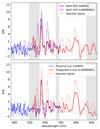 |
Fig. 2 Cross-correlation S/N between the ExoMol VO line list and M-dwarf spectra for each UVES-sized spectral order. The solid and dotted lines depict the observed and injected signals, respectively. Top panel: cross-correlation with the HARPS and CARMENES spectra of Wolf 359. Bottom panel: cross-correlation with the HARPS spectrumof Proxima Centauri and the CARMENES spectrum of Teegarden’s star. The grey vertical bands are regions which are not covered by the UVES spectrograph. |
2.4 Selection of accurate lines
Instead of using every quantum state in the VO line list, we also made models solely involving the well-constrained energy levels. Consequently, the inaccurate spectral lines are excluded and the model spectrum is a more accurate, but incomplete representation of the real VO absorption. The quantum states listed in Table 1 were included in our reduced line list. These energy levels were refined with experimental data (McKemmish et al. 2016, Table 3) and the spectroscopic model managed to fit the empirical energy levels relatively well with RMS(ω) ≲ 0.3 cm−1‚ which corresponds to RMS(vrad) ≲ 6 km s−1 at 700 nm. Transitions from the X4Σ− ground state to the excited B4Π or C4Σ− states were included in the new reduced line list. This state selection decreases the number of transitions to 8008 between 669 unique upper states and 388 unique lower states. ExoCross was then run with a specific selection of transitions to generate the opacity data for petitRADTRANS. The computed opacity data are available in the petitRADTRANS archive5 as ‘VO_ExoMol_Specific_Transitions’.
In the model spectrum generated with the complete line list, the large number of spectral lines caused a pseudo-continuum to form below the blackbody profile, decreasing the individual line depths. Since the reduced line list did not produce a similar pseudo-continuum, its spectral lines appeared deeper and this would have affected the cross-correlation if we had not performed a correction. The opacity cross sections of the reduced line list were subtracted from the complete line list, resulting in the opacities of the non-selected transitions. petitRADTRANS used the same configuration described in Sect. 2.1 to generate a model spectrum of the non-selected transitions. Subsequently, we divided the complete model spectrum by the non-selected spectrum, generating a normalised model spectrum for the reduced line list including a correction for the line depths. As in Sect. 2.3, before cross-correlating, a high-pass filter was applied to the normalised model spectrum using a 5 Å-wide Gaussian kernel. The grey spectrum in the bottom panel of Fig. 1 shows the normalised model spectrum of the reduced line list. Many of the strongest spectral lines in the bandheads around 580, 620, 750, 800, and 870 nm are included in the state-selection model spectrum.
The spectrum derived from the reduced line list was cross-correlated with the spectra of Wolf 359 where the complete VO model was injected. The integrated CCF was obtained using the same method described in Sect. 2.3 and is shown in Fig. 3 as a solid red line. The injected signal has an S/N of 11.0σ, which is lower than that obtained with the complete line list (12.3σ). This is expected because the injected signal was recovered with substantially fewer spectral lines. On the other hand, the S/N of the observed signal has increased from 5.9σ to 9.9σ, which confirms an improved accuracy by about a factor 1.8 for the reduced line list. The observed-to-injected signal ratio using the reduced line list was calculated to be (S/N)obs/(S/N)inj = 0.90. Hence, a cross-correlation analysis using the UVES-sized spectral orders and the reduced VO line list retrieves 90% of the potential signal from these M-dwarf spectra (reducing the signal by a factor 1.1), requiring 1.12 = 1.2 times more observing time. Additionally, we performed a cross-correlation with the non-selected lines to confirm that most of the accurate lines were included in the reduced line list. The total CCF of the non-selected lines with the spectra of Wolf 359 is shown as the red dotted line in Fig. 3. Since the observed signal measures at only 0.5σ, we conclude that the non-selected transitions contribute to reducing the cross-correlation performance of the complete line list.
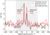 |
Fig. 3 Combined CCFs from every UVES-sized order after the VO injection. The black line shows the CCF using the complete VO line list. The solid and dotted red lines show the CCF using the reduced line list described in Sect. 2.4 and the CCF using the non-selected transitions, respectively. The grey region depicts the excluded velocity range used to determine the noise level in the CCF. The peaks at −25 and 0 km s−1 are the injected and observed signals, respectively. |
Well-defined energy levels of VO (McKemmish et al. 2016) included in the reduced line list.
3 Analysis of WASP-121b transmission spectra
The M-dwarf analysis allowed us to determine the cross-correlation performance of the ExoMol VO line list, and to test the selection of specific transitions, increasing the VO detection significance. Subsequently, we aimed to confirm the presence of VO in the transmission spectrum of WASP-121b at high spectral resolution using the complete and reduced line list. Evidence for VO has been presented at low spectral resolution in the literature (Evans et al. 2016, Evans et al. 2018; Mikal-Evans et al. 2019). WASP-121b orbits a bright F6V-type star (V = 10.5; Høg et al. 2000) with a short orbital period of 1.27 days (Delrez et al. 2016). The parameters of the WASP-121 system utilised in this paper are listed in Table 2. We used the same UVES transmission spectra previously presented by Gibson et al. (2020), and Merritt et al. (2020, 2021). While Merritt et al. (2020) used only the UVES red arm data for their non-detections of TiO and VO, our analysis used both the blue and red arms. The spectral resolution of the data was R ~ 80000 for the blue arm and R ~ 110000 for the red arm. A more detailed description of the data as well as an outline of the custom calibration pipeline can be found in Merritt et al. (2020). The pipeline places the spectra on a common wavelength grid and shifts the spectra to the stellar rest frame by correcting for the barycentric and systemic velocity. The stellar reflex motion is not accounted for because the stellar velocity semi-amplitude (K* = 0.181 km s−1; Delrez et al. 2016) is significantly smaller than the resolution of the UVES spectrograph (~2.7 km s−1 at R ~ 110000).
The variation of the blaze function was removed with the same method as Merritt et al. (2020). Since the blaze correction was found to be unstable at the edges of each spectral order, we removed the first 600 pixels and last 60 pixels of each order in the blue arm (22% of pixels; Gibson et al. 2020), as well as the first 500 pixels from the red arm’s orders (12% of pixels; Merritt et al. 2020). We determined common features between the 134 spectra with principal-component analysis (PCA). Injection tests enabled us to determine that subtracting the first eight PCs removed the (quasi)-static stellar or telluric features sufficiently.
System parameters of WASP-121b and its host star as used in this paper.
3.1 Model transmission spectra
The petitRADTRANS radiative transfer code (Mollière et al. 2019) was used to make model transmission spectra of VO in WASP-121b’s atmosphere. The utilised model parameters are listed in Table 2. As in Merritt et al. (2020), we used the same temperatures and cloud deck, and we assumed isothermal atmospheres with 100 atmospheric layers. Twelve constant VO volume-mixing ratios were tested, including VMR [VO] = 10−6.6 as reported by Evans et al. (2018). Rayleigh scattering from H2 and continuum absorption by H− were included. The necessary abundances of H2, H and e− were produced by the petitRADTRANS chemical equilibrium table (VMR [H2] = 0.2, VMR [H] = 0.1, VMR [e−] = 2.1 × 10⁻¹⁰) and we used the volume-mixing ratio of Evans et al. (2018) for H− (VMR [H−] = 5 × 10⁻¹⁰). A mean molecular weight of 2.33 was used and the model spectra were rotationally broadened following the method of Brogi et al. (2016) with veq = 7.1 km s−1, which was inferred by assuming tidal locking. The instrumental broadening was also accounted for with a Gaussian filter set by the resolution of the respective UVES arms. Using the same procedure outlined in Sect. 2.4, we performed a pseudo-continuum correction to obtain transmission spectra of the reduced line list with the appropriate line depths. Figure A.1 shows a comparison between the transmission spectra with different scale heights and temperatures. Before performing the cross-correlation analysis, the low-frequency structure was removed from each model transmission spectrum by dividing a smoothed spectrum, which was obtained by convolution with a 5 Å-wide Gaussian kernel. This normalisation of the model spectra was performed because the low-frequency structure in the observed data was removed by the detrending.
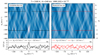 |
Fig. 4 Cross-correlation analysis of WASP-121b’s UVES transmission spectra, using the model parameters reported by Evans et al. (2018). Left panels: analysis with the complete line list and the right panels use the reduced line list described in Sect. 2.4. Top panels: Kp-υsγs maps and the bottom panels show horizontal slices of these maps at the expected planet velocity Kp = 217 km s−1 (dashed) and at the injection velocity Kp = −217 km s−1 (solid). |
3.2 Cross-correlation
Using the weighted cross-correlation function from Eq. (11) in Brogi & Line (2019), each spectrum of each order was cross-correlated with the model transmission spectra with radial velocities ranging from −600 to +600 km s−1 in steps of 0.5 km s−1. The out-of-transit spectra do not contain a planetary signal and the signal is weaker for the frames during ingress and egress. The varying signal strength was accounted for by weighting the CCFs with a PyTransit (Parviainen 2015) model light curve using the equations of Mandel & Agol (2002) with limb-darkening coefficients c1 = 0.395 and c2 = 0.141 (Wilson et al. 2021). We note that VO is absent in the stellar atmosphere due to WASP-121’s high effective temperature (6459 ± 140 K; Delrez et al. 2016), and thus we did not encounter the Rossiter-McLaughlin effect or centre-to-limb variation. Following the integration steps described in Merritt et al. (2020), a Kp-vsγs map of cross-correlation coefficients was constructed for each evaluated model. A coefficient was calculated for planet velocities Kp ranging from −400 to +400 km s−1 in steps of 1 km s−1 and systemic velocities vsγs ranging from −200 to +200 km s−1 in steps of 1 km s−1. The Kp-vsγs maps were converted into detection S/Ns by dividing with the standard deviation of two rectangles outside of the expected peak (Kp from +100 to +300 km s−1 and vsys from −200 to −50 or from +50 to +200 km s−1). We set our detection threshold at 4σ, since we made a simple noise estimation and noise fluctuations of the Kp-vsγs maps could therefore be misinterpreted as detections with a lower threshold (Cabot et al. 2018).
3.3 Results and injection tests
In agreement with Merritt et al. (2020), our cross-correlation analysis failed to retrieve a significant signal around the expected velocities (Kp ~ 217 km s−1 and vsγs ~ 0 km s−1) with any of the evaluated configurations of VMR and T. Furthermore, our reduced line list did not yield a VO detection around the expected Kp and vsys with any of the model spectra. Figure 4 displays the Kp-vsys maps of both assessed line lists for the atmosphere reported by Evans et al. (2018) (VMR = 10−66, T = 1500 K, and a derived scale height of H = 540 km). The colourbar and the dashed CCFs in the bottom panels demonstrate that neither line list recovers a signal exceeding the 4σ detection threshold around the expected Kp and vsys.
Injection tests were carried out to determine whether a VO transmission signal could be detected with our retrieval method. The injection was performed by multiplying the UVES spectra with the complete model transmission spectra before applying the blaze correction. The varying signal strength was accounted for by scaling the models with the same PyTransit (Parviainen 2015) light curve described in Sect. 3.2. The models were injected at Kp = −217 km s−1 to avoid the enhancement by any undetected, real VO signal. Figure 4 displays the Kp-vsγs maps around the injected signal and the solid CCFs in the bottom panels show the horizontal slices at Kp = −217 km s−1. The retrieval with the complete line list yields a detectable signal of 4.5σ. However, we emphasise that this injection test assumes a perfect line list as the cross-correlation template is identical to the injected model. Section 2.3 demonstrates that this assumption is incorrect and that we need to correct for the inaccuracies of the ExoMol VO line list. Similar to the M-dwarf injection test of Sect. 2.4, the reduced line list recovers a lower injected signal from the UVES spectra as a consequence of the decreased number of lines.
Figure 5 displays the detection significance of the injected signal as a function of the log10 VO volume-mixing ratio. The leftmost panel shows the recovered signal using the complete VO line list. As expected, higher temperatures (indicated by the dark blue lines) increase the atmospheric scale height, which in turn increases the detection significance. Our more extensive treatment of rotational broadening decreases the detection S/Ns compared to analogous models (e.g. T = 1500 K and H = 550 km) in Fig. 6 in Merritt et al. (2020). The results of the injection tests are more similar to those of Merritt et al. (2020) when the effects of rotation are disregarded. Many evaluated models exceed the 4σ detection limit and should therefore be detectable. However, Sect. 2.3 demonstrates that the ExoMol VO line list is imperfect and only 48% of an optimal, injected cross-correlation signal could be recovered from M-dwarf Wolf 359’s spectrum. We utilised the derived cross-correlation performance to simulate the reduction of the signal recovered from the WASP-121b data caused by the line list’s inaccuracies. The second panel of Fig. 5 shows the injected VO signal multiplied by 0.48. The injected signal no longer exceeds the 4σ detection limit with the parameters reported by Evans et al. (2018). In fact, the re-scaled VO signal is not detectable for T = 1500 and 2000 K with any of the evaluated abundances. Hence, it appears unlikely that the low-resolution VO detection by Evans et al. (2018) (T = 1500 K, VMR = 10−6.6) can be confirmed with these UVES spectra and the current VO line list. Via interpolation, we find that abundances higher than VMR = 10−6 8 exceed the detection threshold for T = 3000 K. However, at this temperature thermal dissociation is expected to decrease the VO abundance to ≲ 10−10 (Merritt et al. 2020).
The third panel of Fig. 5 shows the recovered signal using the reduced line list and the rightmost figure shows the same signal multiplied by the observed-to-injected signal ratio for the reduced line list (Sect. 2.4; (S/N)obs/(S/N)inj = 0.90). In contrast with the complete line list, the cross-correlation signal is not increased two-fold by a doubling of the scale height (H = 540 and 1080 km) following an increase in the temperature (T = 1500 and 3000 K). We diagnosed that this discrepancy is an inherent property of our reduced line list. The light green line in Fig. 5 displays the injected signal obtained with model transmission spectra where we artificially set the scale height to H = 1080 km (by adjusting the surface gravity in petitRAD-TRANS) for a temperature of T = 1500 K. For these models, the detection significances show an approximate two-fold increase over the H = 540 km models, caused by the increased depths of the absorption lines. On the other hand, a higher temperature causes the lines selected in our reduced line list to generally become shallower as a consequence of rising collisional excitations. The relatively low-lying states in our reduced line list become less populated and the opacity of their transitions therefore decreases. The dark green line in Fig. 5 displays models with a heightened temperature of T = 3000 K for a scale height of H = 540 km. The injected signal is substantially decreased due to the temperature effect. The increase brought about by the scale height and the decrease caused by the temperature effect yield a negligible improvement in the detection significance retrieved by our reduced line list for a rising temperature. The cancellation is also found in the bottom panel of Fig. A.1, where the bands that are used in the reduced line list have similar depths for T = 1500 and 3000 K. The complete line list retrieves an increased cross-correlation signal because the weaker lines involving the excited states become deeper by an increased temperature (e.g. ~600 nm in Fig. A.1). From Fig. 5 we deduce that the reduced line list could not detect VO even if we assumed it to be perfect. Consequently, the evaluated models are not detectable after accounting for the reduced line list’s inaccuracies. Therefore, our reduced line list also appears unsuited for detecting a VO signal in the transmission spectra of WASP-121b.
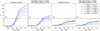 |
Fig. 5 Detection significance of the injected signal versus log10 VMR for each model configuration. Left panel: recovered signal using all quantum transitions. Second panel: same signal multiplied by 0.48 as found in Sect. 2.1. Third panel: recovered signal using specific quantum transitions and the fourth panel shows the same signal multiplied by 0.90 as obtained in Sect. 2.4. The considered temperatures are displayed as different shades of blue. Two rightmost panels: detection significances of models with T = 1500 K, H = 1080 km, and T = 3000 K, H = 540 km in light green and dark green, respectively. The horizontal dashed lines at 4σ represent our detection thresholds. |
4 Discussion and conclusions
We have presented a quantitative assessment of the ExoMol VO line list using high-resolution HARPS and CARMENES spectra of M-dwarfs. The injection of a Doppler-shifted peti-tRADTRANS model spectra of VO allowed us to compare the cross-correlation performance of the injected, optimal signal against the observed signal. The line list performs well around the absorption bands at ~580 and ~800 nm due to the availability of experimental data used in refining the computed energy levels (McKemmish et al. 2016). Future work could focus on updating the vibrationally excited levels to improve the quality of the VO line list. We find that a cross-correlation analysis recovers only 48% of the potential signal. Furthermore, we made a reduced VO line list which only included the most accurate energy levels. While this line list is an incomplete representation of the actual VO opacity, it achieves a higher cross-correlation signal in M-dwarfs by a factor of 1.8 compared to the complete line list. The reduced line list manages to recover 90% of the optimal signal. We have presented non-detections of VO in the UVES transmission spectrum of WASP-121b using the complete and reduced line list. After accounting for the line list’s performance, injection tests showed that our retrieval method would likely not detect VO if it were present in the abundance reported by Evans et al. (2018). This analysis appears to confirm that the VO non-detections from Hoeijmakers et al. (2020) and Merritt et al. (2020) are indeed inconclusive due to the inaccuracies of the ExoMol VO line list.
Recently, the ExoMol group released an updated TiO line list (McKemmish et al. 2019)6 after it was shown that the previous line lists were insufficient to retrieve a TiO cross-correlation signal in M-dwarf spectra (Hoeijmakers et al. 2015; Nugroho et al. 2017). The MARVEL algorithm (Furtenbacher & Császár 2012) analyses collated experimental data of TiO to determine experimental-accuracy energy levels. The TiO energy levels which had been computed using quantum chemistry were subsequently replaced with the MARVEL-produced energies. The updated TiO line list showed an improved performance when cross-correlating with high-resolution M-dwarf spectra. This MARVEL-isation has not yet been applied to the VO line list, but we note that work is currently underway in the ExoMol group to produce a high-resolution line list for VO which makes use of MARVEL energy levels (Jonathan Tennyson, priv. comm.). We expect such an update to greatly improve the ability to find this species in exoplanet atmospheres.
Acknowledgements
The authors would like to thank the HARPS consortium and CARMENES consortium for making their data publicly available. This work was further based on data retrieved at the European Organisation for Astronomical Research in the Southern Hemisphere as part of ESO program 098.C-0547. This work was performed using the ALICE compute resources provided by Leiden University. This work made use of the following software packages that were not referenced in the main text: NumPy, SciPy, AstroPy, Matplotlib, iPython and Pandas (van der Walt et al. 2011; Virtanen et al. 2020; Astropy Collaboration 2018; Hunter 2007; Pérez & Granger 2007; The pandas development team 2020). I.S. and A.K. acknowledge funding from the European Research Council (ERC) under the European Union’s Horizon 2020 research and innovation program under grant agreement No 694513.
Appendix A Model transmission spectra
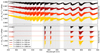 |
Fig. A.1 Examples of VO model transmission spectra using an abundance of VMR = 10−6.6. The top panel shows the spectra generated with the complete line list and the bottom panel used the pseudo-continuum correction described in Sect. 2.4 to create transmission spectra of the reduced line list. The four temperatures used in the presented analysis are shown with different colours and are offset for easier comparison. The grey vertical bands in both panels show the wavelength ranges of the UVES spectral orders. |
References
- Astropy Collaboration (Price-Whelan, A.M., et al.) 2018, AJ, 156, 123 [NASA ADS] [CrossRef] [Google Scholar]
- Birkby, J. L., de Kok, R. J., Brogi, M., et al. 2013, MNRAS, 436, L35 [Google Scholar]
- Bourrier, V., Kitzmann, D., Kuntzer, T., et al. 2020, A&A, 637, A36 [NASA ADS] [CrossRef] [EDP Sciences] [Google Scholar]
- Brogi, M., & Line, M. R. 2019, AJ, 157, 114 [Google Scholar]
- Brogi, M., Snellen, I. A. G., de Kok, R. J., et al. 2012, Nature, 486, 502 [Google Scholar]
- Brogi, M., Kok, R. J. D., Albrecht, S., et al. 2016, ApJ, 817, 106 [NASA ADS] [CrossRef] [Google Scholar]
- Cabot, S. H. C., Madhusudhan, N., Hawker, G. A., & Gandhi, S. 2018, MNRAS, 482, 4422 [Google Scholar]
- Czesla, S., Schröter, S., Schneider, C. P., et al. 2019, PyA: Python astronomy-related packages, Astrophysics Source Code Library, [record ascl:1986.818] [Google Scholar]
- Daylan, T., Günther, M. N., Mikal-Evans, T., et al. 2021, AJ, 161, 3 [NASA ADS] [Google Scholar]
- Delrez, L., Santerne, A., Almenara, J. M., et al. 2016, MNRAS, 458, 4025 [NASA ADS] [CrossRef] [Google Scholar]
- Evans, T. M., Sing, D. K., Wakeford, H. R., et al. 2016, ApJ, 822, L4 [NASA ADS] [CrossRef] [Google Scholar]
- Evans, T. M., Sing, D. K., Kataria, T., et al. 2017, Nature, 548, 58 [NASA ADS] [CrossRef] [Google Scholar]
- Evans, T. M., Sing, D. K., Goyal, J. M., et al. 2018, AJ, 156, 283 [NASA ADS] [CrossRef] [Google Scholar]
- Fortney, J., Lodders, K., Marley, M., & Freedman, R. 2008, ApJ, 678, 1419 [CrossRef] [Google Scholar]
- Furtenbacher, T., & Császár, A. G. 2012, J. Quant. Spectr. Rad. Transf., 113, 929 [NASA ADS] [CrossRef] [Google Scholar]
- Gaia Collaboration 2018, VizieR Online Data Catalog: I/345 [Google Scholar]
- Gharib-Nezhad, E., & Line, M. R. 2019, ApJ, 872, 27 [NASA ADS] [CrossRef] [Google Scholar]
- Gibson, N. P., Merritt, S., Nugroho, S. K., et al. 2020, MNRAS, 493, 2215 [Google Scholar]
- Gustafsson, B., Edvardsson, B., Eriksson, K., et al. 2008, A&A, 486, 951 [NASA ADS] [CrossRef] [EDP Sciences] [Google Scholar]
- Hoeijmakers, H. J., de Kok, R. J., Snellen, I. A. G., et al. 2015, A&A, 575, A20 [NASA ADS] [CrossRef] [EDP Sciences] [Google Scholar]
- Hoeijmakers, H. J., Seidel, J. V., Pino, L., et al. 2020, A&A, 641, A123 [NASA ADS] [CrossRef] [EDP Sciences] [Google Scholar]
- Høg, E., Fabricius, C., Makarov, V. V., et al. 2000, A&A, 355, L27 [Google Scholar]
- Hubeny, I., Burrows, A., & Sudarsky, D. 2003, ApJ, 594, 1011 [Google Scholar]
- Hunter, J. D. 2007, Comput. Sci. Eng., 9, 90 [NASA ADS] [CrossRef] [Google Scholar]
- Kesseli, A. Y., Kirkpatrick, J. D., Fajardo-Acosta, S. B., et al. 2019, AJ, 157, 63 [Google Scholar]
- Kirkpatrick, J. D., Reid, I. N., Liebert, J., et al. 1999, ApJ, 519, 802 [NASA ADS] [CrossRef] [Google Scholar]
- Landolt, A. U. 1992, AJ, 104, 340 [Google Scholar]
- Lothringer, J. D., & Barman, T. 2019, ApJ, 876, 69 [Google Scholar]
- Mandel, K., & Agol, E. 2002, ApJ, 580, L171 [Google Scholar]
- Mayor, M., Pepe, F., Queloz, D., et al. 2003, The Messenger, 114, 20 [NASA ADS] [Google Scholar]
- McKemmish, L. K., Yurchenko, S. N., & Tennyson, J. 2016, MNRAS, 463, 771 [NASA ADS] [CrossRef] [Google Scholar]
- McKemmish, L. K., Masseron, T., Sheppard, S., et al. 2017, ApJS, 228, 15 [NASA ADS] [CrossRef] [Google Scholar]
- McKemmish, L. K., Masseron, T., Hoeijmakers, H. J., et al. 2019, MNRAS, 488, 2836 [Google Scholar]
- Merritt, S. R., Gibson, N. P., Nugroho, S. K., et al. 2020, A&A, 636, A117 [NASA ADS] [CrossRef] [EDP Sciences] [Google Scholar]
- Merritt, S. R., Gibson, N. P., Nugroho, S. K., et al. 2021, MNRAS, 506, 3853 [NASA ADS] [CrossRef] [Google Scholar]
- Mikal-Evans, T., Sing, D. K., Goyal, J. M., et al. 2019, MNRAS, 488, 2222 [Google Scholar]
- Mikal-Evans, T., Sing, D. K., Kataria, T., et al. 2020, MNRAS, 496, 1638 [Google Scholar]
- Mollière, P., van Boekel, R., Bouwman, J., et al. 2017, A&A, 600, A10 [Google Scholar]
- Mollière, P., Wardenier, J. P., van Boekel, R., et al. 2019, A&A, 627, A67 [Google Scholar]
- Nakajima, T., & Sorahana, S. 2016, ApJ, 830, 159 [NASA ADS] [CrossRef] [Google Scholar]
- Nugroho, S. K., Kawahara, H., Masuda, K., et al. 2017, AJ, 154, 221 [Google Scholar]
- Parviainen, H. 2015, MNRAS, 450, 3233 [Google Scholar]
- Pavlenko, Y. V., Jones, H. R. A., Lyubchik, Y., Tennyson, J., & Pinfield, D. J. 2006, A&A, 447, 709 [NASA ADS] [CrossRef] [EDP Sciences] [Google Scholar]
- Pérez, F., & Granger, B. E. 2007, Comput. Sci. Eng., 9, 21 [Google Scholar]
- Quirrenbach, A., Amado, P. J., Ribas, I., et al. 2018, SPIE, 10702, 246 [Google Scholar]
- Reiners, A., Zechmeister, M., Caballero, J. A., et al. 2018, A&A, 612, A49 [NASA ADS] [CrossRef] [EDP Sciences] [Google Scholar]
- Ribas, I., Gregg, M. D., Boyajian, T. S., & Bolmont, E. 2017, A&A, 603, A58 [NASA ADS] [CrossRef] [EDP Sciences] [Google Scholar]
- Sing, D. K., Lavvas, P., Ballester, G. E., et al. 2019, AJ, 158, 91 [Google Scholar]
- Snellen, I. A. G., de Kok, R. J., de Mooij, E. J. W., & Albrecht, S. 2010, Nature, 465, 1049 [Google Scholar]
- Tennyson, J., Lodi, L., McKemmish, L. K., & Yurchenko, S. N. 2016, J. Phys. B, 49, 102001 [NASA ADS] [CrossRef] [Google Scholar]
- Tennyson, J., Yurchenko, S. N., Al-Refaie, A. F., et al. 2020, J. Quant. Spectr. Rad. Transf., 255, 107228 [NASA ADS] [CrossRef] [Google Scholar]
- The pandas development team 2020, https://doi.org/10.5281/zenodo.3509134 [Google Scholar]
- van der Walt, S., Colbert, S.C., & Varoquaux, G. 2011, Comput. Sci. Eng., 13, 22 [NASA ADS] [CrossRef] [Google Scholar]
- Virtanen, P., Gommers, R., Oliphant, T. E., et al. 2020, Nat. Methods, 17, 261 [Google Scholar]
- Wilson, J., Gibson, N. P., Lothringer, J. D., et al. 2021, MNRAS, 503, 4787 [NASA ADS] [CrossRef] [Google Scholar]
- Yurchenko, S. N., Al-Refaie, A. F., & Tennyson, J. 2018, A&A, 614, A131 [NASA ADS] [CrossRef] [EDP Sciences] [Google Scholar]
Calar Alto high-Resolution search for M-dwarfs with Exoearths with Near-infrared and optical Echelle Spectrographs.
This line list was updated in August 2021 to correct an error which had been identified in the MARVEL process for TiO; the latest version number is 20210825, as can be found in the Exo-Mol.def file, https://www.exomol.com/db/TiO/48Ti-16O/Toto/48Ti-16O__Toto.def
All Tables
Well-defined energy levels of VO (McKemmish et al. 2016) included in the reduced line list.
All Figures
|
Fig. 1 Comparison between the observed M-dwarf spectra and the petitRADTRANS VO model spectra. Top panel: HARPS and CARMENES spectra of Wolf 359 in blue and red, respectively. Bottom panel: normalised VO model spectra using all quantum transitions in black and using the specific transitions described in Sect. 2.4 in grey. The grey vertical bands in both panels show the wavelength ranges of the UVES spectral orders. |
| In the text | |
|
Fig. 2 Cross-correlation S/N between the ExoMol VO line list and M-dwarf spectra for each UVES-sized spectral order. The solid and dotted lines depict the observed and injected signals, respectively. Top panel: cross-correlation with the HARPS and CARMENES spectra of Wolf 359. Bottom panel: cross-correlation with the HARPS spectrumof Proxima Centauri and the CARMENES spectrum of Teegarden’s star. The grey vertical bands are regions which are not covered by the UVES spectrograph. |
| In the text | |
|
Fig. 3 Combined CCFs from every UVES-sized order after the VO injection. The black line shows the CCF using the complete VO line list. The solid and dotted red lines show the CCF using the reduced line list described in Sect. 2.4 and the CCF using the non-selected transitions, respectively. The grey region depicts the excluded velocity range used to determine the noise level in the CCF. The peaks at −25 and 0 km s−1 are the injected and observed signals, respectively. |
| In the text | |
|
Fig. 4 Cross-correlation analysis of WASP-121b’s UVES transmission spectra, using the model parameters reported by Evans et al. (2018). Left panels: analysis with the complete line list and the right panels use the reduced line list described in Sect. 2.4. Top panels: Kp-υsγs maps and the bottom panels show horizontal slices of these maps at the expected planet velocity Kp = 217 km s−1 (dashed) and at the injection velocity Kp = −217 km s−1 (solid). |
| In the text | |
|
Fig. 5 Detection significance of the injected signal versus log10 VMR for each model configuration. Left panel: recovered signal using all quantum transitions. Second panel: same signal multiplied by 0.48 as found in Sect. 2.1. Third panel: recovered signal using specific quantum transitions and the fourth panel shows the same signal multiplied by 0.90 as obtained in Sect. 2.4. The considered temperatures are displayed as different shades of blue. Two rightmost panels: detection significances of models with T = 1500 K, H = 1080 km, and T = 3000 K, H = 540 km in light green and dark green, respectively. The horizontal dashed lines at 4σ represent our detection thresholds. |
| In the text | |
|
Fig. A.1 Examples of VO model transmission spectra using an abundance of VMR = 10−6.6. The top panel shows the spectra generated with the complete line list and the bottom panel used the pseudo-continuum correction described in Sect. 2.4 to create transmission spectra of the reduced line list. The four temperatures used in the presented analysis are shown with different colours and are offset for easier comparison. The grey vertical bands in both panels show the wavelength ranges of the UVES spectral orders. |
| In the text | |
Current usage metrics show cumulative count of Article Views (full-text article views including HTML views, PDF and ePub downloads, according to the available data) and Abstracts Views on Vision4Press platform.
Data correspond to usage on the plateform after 2015. The current usage metrics is available 48-96 hours after online publication and is updated daily on week days.
Initial download of the metrics may take a while.