| Issue |
A&A
Volume 661, May 2022
|
|
|---|---|---|
| Article Number | A71 | |
| Number of page(s) | 13 | |
| Section | Cosmology (including clusters of galaxies) | |
| DOI | https://doi.org/10.1051/0004-6361/202142162 | |
| Published online | 05 May 2022 | |
High-redshift cosmography: Application and comparison with different methods
1
School of Astronomy and Space Science, Nanjing University, Nanjing 210093, PR China
e-mail: This email address is being protected from spambots. You need JavaScript enabled to view it.
2
Key Laboratory of Modern Astronomy and Astrophysics (Nanjing University), Ministry of Education, Nanjing 210093, PR China
Received:
6
September
2021
Accepted:
15
February
2022
Abstract
Cosmography is used in cosmological data processing in order to constrain the kinematics of the universe in a model-independent way. In this paper, we first investigate the effect of the ultraviolet (UV) and X-ray relation of a quasar on cosmological constraints. By fitting the quasar relation and cosmographic parameters simultaneously, we find that the 4σ deviation from the cosmological constant Λ cold dark matter (ΛCDM) model disappears. Next, utilizing the Pantheon sample and 31 long gamma-ray bursts, we make a comparison among the different cosmographic expansions (z-redshift, y-redshift, E(y), log(1 + z), log(1 + z)+kij, and Padé approximations) with the third-order and fourth-order expansions. The expansion order can significantly affect the results, especially for the y-redshift method. Through analysis from the same sample, the lower-order expansion is preferable, except the y-redshift and E(y) methods. For the y-redshift and E(y) methods, despite adopting the same parameterization of y = z/(1 + z), the performance of the latter is better than that of the former. Logarithmic polynomials, log(1 + z) and log(1 + z)+kij, perform significantly better than z-redshift, y-redshift, and E(y) methods, but worse than Padé approximations. Finally, we comprehensively analyze the results obtained from different samples. We find that the Padé(2,1) method is suitable for both low and high redshift cases. The Padé(2,2) method performs well in a high-redshift situation. For the y-redshift and E(y) methods, the only constraint on the first two parameters (q0 and j0) is reliable.
Key words: cosmological parameters / quasars: general / gamma-ray burst: general / supernovae: general
© ESO 2022
1. Introduction
Cosmography has been widely used to restrict the state of the kinematics of our universe employing measured distances (Visser 2015; Dunsby & Luongo 2016; Capozziello et al. 2019, 2020). It is a model-independent strategy which only relies on the assumption of a homogeneous and isotropic universe which is described by the Friedman-Lemaitre-Robertson-Walker (FLRW) metric well (Weinberg 1972). Its methodology is essentially based on expanding a measurable cosmological quantity into the Taylor series around the present time. In the beginning, the luminosity distance was expanded into a z-redshift series which estimated the cosmic evolution at z ∽ 0 well, but it failed at high redshifts (Chiba & Nakamura 1998; Caldwell & Kamionkowski 2004; Riess et al. 2004; Visser 2004). The poor performance at high redshifts of the z-redshift expansion strongly affects the results (Vitagliano et al. 2010). Cattoën & Visser (2007) pointed out that the lack of validity of the Taylor expansions for the luminosity distance could settle down at approximately z ∽ 1. However, there are two main problems associated with the use of the above expansion and analysis of the cosmic data (Capozziello et al. 2020). One is the inability to distinguish the evolution of dark energy from the cosmological constant Λ. Higher precise redshift data found from future surveys will be helpful to address this problem (D’Agostino & Nunes 2019; Bonilla et al. 2020; Lusso 2020). The other issue is the convergence problem caused by data that are far from the limits of Taylor expansions, leading to a severe error propagation, which reduces the cosmography predictions (Cattoën & Visser 2007; Busti et al. 2015). In order to solve this problem, several approaches have been proposed. According to the construction method, it can be divided into two categories. One would be using the auxiliary variables to reparameterize the redshift variable through functions of z, for example y-redshift (Chevallier & Polarski 2001; Linder 2003) and E(y) (Rezaei et al. 2020). The other way would be to consider a smooth evolution of the involved observables by expanding them in terms of rational approximation, for example Padé (Gruber & Luongo 2014; Wei et al. 2014; Capozziello et al. 2020) and Chebyshev rational polynomials (Shafieloo 2012; Capozziello et al. 2018a).
In order to avoid the convergent problem of the series at high redshifts, it is better to replace the parameter z with y = z/(1 + z) (Chevallier & Polarski 2001; Linder 2003; Vitagliano et al. 2010). By making such a transformation, z ∈ (0, ∞) can be mapped into y∈ (0, 1). In theory, employing the y-redshift series method, high-redshift observations could be used for cosmology, that is, type Ia supernovae (SNe Ia), gamma-ray bursts (GRBs), and quasars. However, Zhang et al. (2017) found that both the z-redshift and y-redshift methods have a small biased estimation by employing the Joint Light-curve Analysis (JLA) sample (Betoule et al. 2014) and combining the bias-variance tradeoff. It means that Taylor expansion can describe the SNe Ia well. Whilst they also found that a y-redshift produces larger variances beyond the second-order expansion. Then based on the y-redshift expansion, Rezaei et al. (2020) attempted to recast E(z) as a function of y = z/(1 + z) and they adopted the new series expansion of the E(y) function to compare dark energy models. From the numerical results, they found that the restriction on two of the cosmological parameters, deceleration parameter q0 and jerk parameter j0, are much tighter than that of other two parameters s0 and l0. This point is in line with the previous claim of Zhang et al. (2017). Thus replacing a z-redshift with a y-redshift may only alleviate the divergence when z tends to infinity and it could not completely solve the convergence problem. In recent works (Lusso et al. 2019; Risaliti & Lusso 2019), a new expansion of the luminosity distance-redshift relation in terms of the logarithmic polynomials has been used for cosmography. In such a way, a z-redshift was replaced by log(1 + z). Employing the logarithmic polynomials, Risaliti & Lusso (2019) found a 4σ tension with the ΛCDM model from a high-redshift Hubble diagram of SNe Ia and quasars. Lusso et al. (2019) confirmed this tension with SNe Ia, GRBs and quasars using two model-independent methods (y-redshift and the logarithmic polynomials). After that, Bargiacchi et al. (2021) improved a new logarithmic polynomial expansion by introducing orthogonal terms. This new method and the corresponding results have received enough attention (Speri et al. 2021). At the same time, different opinions were voiced (Yang et al. 2020; Banerjee et al. 2021).
Involving the rational approximation, the Padé approximation being the most usual rational approximation method can be regarded as a generalization of the Taylor polynomial. However, it often gives a better approximation of the function than truncating its Taylor series, and it may still work where the Taylar series do not converge (Wei et al. 2014). Until now, due to its excellent convergence properties, the Padé approximation has been widely used in cosmology (Aviles et al. 2014; Demianski et al. 2017; Capozziello & Ruchika Sen 2019; Capozziello et al. 2020). Recently, Capozziello et al. (2020) critically compared the two main solutions of the convergence problem for the first time, that is to say the auxiliary variables (y1 = 1 − a and y2 = arctan(a−1 − 1)) and the Padé approximations. They found that even though y2 overcomes the issues of y1, the most viable approximation of the luminosity distance dL(z) is still given by adopting Padé approximations. In addition, they also investigated two distinct domains involving Monte Carlo analysis on the Pantheon sample, H(z), and shift parameter measurements, and they conclude that the (2,1) Padé approximation is statistically the optimal approach to explain low- and high-redshift data, together with the fifth-order y2-parameterization. At high redshifts, the (2,2) Padé approximation can be essentially ruled out. In addition to the Padé approximation, there are some other methods that can be used in cosmology instead of Taylor expansions, for example Chebyshev series (Capozziello et al. 2018a; Zamora Munõz & Escamilla-Rivera 2020). Until now, there has not been a detailed numerical analysis for the abovementioned six methods (z-redshift, y-redshift, E(y), logarithmic polynomials, orthogonalized logarithmic polynomials, and Padé approximations) using high-redshift data.
In this paper, we try to confirm the effect of the quasar relation on the cosmographic constraint using the Pantheon sample and 1598 quasars in terms of the logarithmic polynomials and the Padé(2,1) approximation. First, we reconsider the parameters γ, β, and δ, which were obtained from the observed quasar relation as free parameters, to explore the situation of 4σ tension. Based on previous research on the Padé approximation (Capozziello et al. 2020), we chose to use the Padé(2,1) method which has excellent convergence to carry out cross checks. A brief introduction to Padé’s excellent convergence has been provided in the previous section. We also compare the Padé(2,1) method with other cosmographic expansions including the logarithmic polynomials combining the Pantheon sample and a new high-redsihft GRB sample including 31 LGRBs (Wang et al. 2022). We also provide a detailed numerical analysis for the different expansions in terms of the values for the Akaike information criterion (AIC) and the Bayesian information criterion (BIC). A fiducial value H0 = 70 km s−1 Mpc−1 is adopted in this paper.
The outline of this paper is as follows. In Sect. 2, we describe the observational data sets that are used in our analyses. Section 3 briefly introduces the different cosmographic approaches and the model selection method. We discuss the effect of the quasar relation on the cosmographic constraints in Sect. 4. The comparison results of different cosmographic approaches are depicted in Sect. 5. Finally, conclusions and discussion are presented in the last section.
2. Observational data sets
2.1. Pantheon
This sample consists 1048 sources covering the redshift range 0.01 < z < 2.26 (Scolnic et al. 2018). This sample, as a set of latest SNe Ia data points, was provided by a number of SN surveys including CfA1-4 (Riess et al. 1999; Jha et al. 2006; Hicken et al. 2009a,b, 2012), the Carnegie supernova (SN) project (CSP; Contreras et al. 2010; Folatelli et al. 2010; Stritzinger et al. 2011), the Sloan Digital Sky Survey (SDSS; Frieman et al. 2008; Kessler et al. 2009; Sako et al. 2018), the Pan-STARRS1 (PS1; Rest et al. 2014; Scolnic et al. 2014), the supernova legacy survey (SNLS; Conley et al. 2011; Sullivan et al. 2011), and the Hubble Space Telescope (HST; Riess et al. 2004, 2007, 2018; Suzuki et al. 2012; Graur et al. 2014; Rodney et al. 2014) SN surveys. According to the redshift range, these surveys have overlapping redshift ranges of 0.01 ≲ z ≲ 0.10 for CfA1-4 and CSP; 0.1 ≲ z ≲ 0.4 for SDSS; 0.103 ≲ z ≲ 0.68 for PS1; 0.3 ≲ z ≲ 1.1 for SNLS; and 1.0 < z for HST. We note that SNe Ia have a nearly uniform intrinsic luminosity with an absolute magnitude around M ∼ − 19.5 (Carroll 2001) which promote it to a well-established class of standard candles. The difficulty in the cosmological applications lies in the identification of absolute magnitude M, due to different sources of systematic and statistical errors. In this work, we only consider the systematic error. The observations used, redshift z, distance modulus μ, and corresponding 1σ error σμ are provided by Scolnic et al. (2018) and can be publicly obtained from the website1. The observational distance modulus μobs(SN) was calculated with the following formula (Tripp 1998),
 (1)
(1)
where α is the coefficient of the relation between the luminosity and stretch, and β is the coefficient of the relation between the luminosity and color. These two parameters were retrieved by using the beams with bias correction (BBC) method. We note that x1 and c are the light-curve shape parameter and the color of the SN, respectively; ΔM is a distance correction based on the host galaxy mass of SN; and ΔB is a distance correlation based on predicted biases from simulations. Furthermore, M is the absolute B-band magnitude of a fiducial SN Ia with x1 = 0 and c = 0. Generally, a standard marginalization over M was performed (Carroll 2001; Betoule et al. 2014; Scolnic et al. 2018).
2.2. GRBs
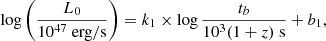
Gamma-ray bursts are promising high-redshift probes (i.e., Wang et al. 2015, 2016; Wei & Wu 2017; Cao et al. 2022; Demianski et al. 2021; Hu et al. 2021). This sample is a compilation of 31 LGRBs ranging from 1.45 < z < 5.91. Similar to SNe Ia, this sample shows a plateau phase caused by the same physical mechanism (Wang et al. 2022). Wang et al. (2022) consider a special case in which the energy injection from electromagnetic dipole emission of millisecond magnetars is larger than the external shock emission. The corresponding light curves of X-ray afterglow show a plateau with a constant luminosity followed by a decay index of about −2 (Dai & Lu 1998; Zhang & Mészáros 2001). The relation between the luminosity L0 and end time tb of the plateau can be well described by the correlation
 (2)
(2)
where log = log10, L0 is the plateau luminosity, tb is the end time of the plateau, and k1 and b1 are two free parameters. Due to the lack of GRBs at low redshifts, the Hubble parameter data constructed by Yu et al. (2018) were used to calibrate the L0–tb correlation via the Gaussian process (GP) method. The calibrated results of the L0–tb correlation are k1 = −1.02 ± 0.12 and b1 = 1.69 ± 0.13. Considering the systematic error σint = 0.22 for the GRB Gold sample, Wang et al. (2022) used the calibrated L0–tb correlation to derive the observational distance modulus μobs and the corresponding errors. In this work, we directly used the results in Table 2 of Wang et al. (2022). We would like to specify that μobs(GRB) and its uncertainty can be derived from (Wang et al. 2022)
 (3)
(3)
and
 (4)
(4)
2.3. Quasars
The quasar sample consists of 1598 objects in the redshift range (0.04, 5.1) with high-quality UV and X-ray flux measurements. The quasar relation between the UV and X-ray emission of quasars can be employed to turn quasars into standard candles, which can be easily described by a formula logLX = γlogLUV + β, where γ and β are two free parameters. This quasar relation has been found from optically and X-ray active galactic nucleus samples with the slope parameter γ around 0.5 to 0.7 (Vignali et al. 2003; Strateva et al. 2005; Steffen et al. 2006; Just et al. 2007; Green et al. 2009; Young et al. 2009, 2010; Jin et al. 2012; Risaliti & Lusso 2015; Lusso & Risaliti 2016; Zhao & Xia 2021). More descriptions about adopting the UV and X-ray correlation of quasars to constrain cosmological parameters can be found in Sect. 4. Due to the lack of quasars at low redshifts, the calibration of parameters γ and β uses other low-redshift observations, that is SNe Ia. Here, we regard them as free parameters and fit them simultaneously with cosmological parameters. The values for z, FUV, FX, and σFUV provided by Risaliti & Lusso (2019) are used.
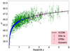 |
Fig. 1. Hubble diagram of SNe Ia, GRBs, and quasars. The picture includes 1048 SNe Ia of the Pantheon sample, 31 LGRBs, and 1598 quasars. The black solid line is a flat ΛCDM model with Ωm = 0.3 and Hubble constant H0 = 70 km s−1 Mpc−1. Distance moduli and corresponding errors are provided by Risaliti & Lusso (2019) which were calculated by the calibrated UV and X-ray correlation using the low-redshift SNe Ia. |
We plot the Hubble diagram of SNe Ia, GRBs, and quasars, as shown in Fig. 1. In discussing the impact of the quasar relation on cosmological constraints, we used the same sample of Risaliti & Lusso (2019), including SNe Ia and quasars, referred to as the SN-Q sample. When comparing different cosmological expansion methods, we use the combined sample. The maximum redshift of 31 LGRBs is higher than that of the Pantheon sample. Therefore, compared to the Pantheon sample, the combined sample can be regarded as a high-redshift sample.
3. Method
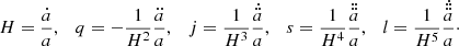
In this section, we briefly introduce the different cosmographic techniques and the model selection method. Cosmography is an artful combination of kinematic parameters by the Taylor expansion with an assumption of large-scale homogeneity and isotropy. In this framework, the evolution of the universe can be described by some cosmographic parameters, such as Hubble parameter H, deceleration q, jerk j, snap s, and lerk l parameters. The definition of them can be expressed as follows:
 (5)
(5)
Initially, the luminosity distance is expanded as z-redshift series (Weinberg 1972; Chiba & Nakamura 1998; Visser 2004). The z-redshift method is completely applicable at z ≪ 1. As the observed redshift increases, the z-redshift exhibits poor behavior which prompts researchers to find new ways to this problem. Many cosmographic approaches have been proposed in order to obtain as much information as possible from higher-redshift observations directly, among which the representative ones are y-redshift, E(y), log(1 + z), log(1 + z) + kij, and Padé approximations. These methods have been widely used in cosmological applications (Wang et al. 2009; Wang & Wang 2014; Wei et al. 2014; Demianski et al. 2017; Capozziello & Ruchika Sen 2019; Yin & Wei 2019; Capozziello et al. 2020; Li et al. 2020; Rezaei et al. 2020; Cai et al. 2022). Next, we briefly introduction these methods.
3.1. Cosmographic expansions
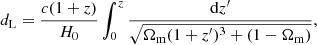
We first introduce the standard model as a guide. Considering the flat ΛCDM model, the luminosity distance dL can be calculated from
 (6)
(6)
where c is the speed of light, H0 is the Hubble constant, and Ωm is the matter density.
z-redshift. The z-redshift method is the earliest Taylor series used in cosmology. The luminosity distance can be conveniently expressed as
![Mathematical equation: $$ \begin{aligned} d_{\mathrm{{L}}}(z) =&\frac{c}{H_{0}}\left[z + \frac{1}{2} (1-q_{0})z^{2} -\frac{1}{6}(1-q_{0}-3q_{0}^{2}+j_{0})z^{3}\right. \nonumber \\& + \frac{1}{24}\left(2-2q_{0}-15q_{0}^{2}-15q_{0}^{3}+5j_{0}+10q_{0}j_{0}+s_{0}\right)z^{4}\nonumber \\& + \frac{1}{120}\Bigg (-6+6q_{0}+81q_{0}^{2}+165q_{0}^{3}+105q_{0}^{4}+10j_{0}^{2}\nonumber \\& -27j_{0}-110q_{0}j_{0}-105q_{0}^{2}j_{0}-15q_{0}s_{0}-11s_{0}-l_{0}\Bigg )z^{5}\nonumber \\& \left.+\textit{O}(z^6)\right], \end{aligned} $$](/articles/aa/full_html/2022/05/aa42162-21/aa42162-21-eq7.gif) (7)
(7)
(Cattoën & Visser 2007; Capozziello et al. 2011), where H0, q0, j0, s0, and l0 are the current values. The first two terms above are Weinberg’s version of the Hubble law which can be found from equation (14.6.8) in the book by Weinberg (1972). The third term and the fourth term are equivalent to that obtained by Chiba & Nakamura (1998) and Visser (2004), respectively.
y-redshift. Mathematically, z-redshift expansion should be performed near a small quantity, that is the low redshift z∽ 0. At that time, with the increase in SN data, the highest redshift was already greater than 1.00. Cattoën & Visser (2007) pointed out that the use of the z-redshift for z > 1 is likely to lead to a convergent problem, that is to say any Taylor series in z is guaranteed to diverge for z > 1. In order to relieve this mathematical problem, they introduced an improved parameterization y = z/(1 + z). The luminosity distance was written as follows:
![Mathematical equation: $$ \begin{aligned} d_{\mathrm{{L}}}({ y}) =&\frac{c}{H_{0}}\left[{ y} - \frac{1}{2}(q_{0} - 3){ y}^{2} + \frac{1}{6}\left(11-5q_{0} + 3q_{0}^{2} - j_{0}\right){ y}^{3}\right.\nonumber \\& + \frac{1}{24}\left(50 - 7j_{0}- 26q_{0} + 10q_{0}j_{0} + 21 q_{0}^{2} - 15q_{0}^{3} + s_{0}\right){ y}^{4} \nonumber \\& + \frac{1}{120}\left(274 - 154q_{0}+141q_{0}^{2}- 135q_{0}^{3} + 105q_{0}^{4} - 47j_{0}\right. \nonumber \\& \left.+ 10j_{0}^{2}+90q_{0}j_{0}-105q_{0}^{2}j_{0}-15q_{0}s_{0}+9s_{0}-l_{0}\right){ y}^5 \nonumber \\& \left.+ \textit{O}({ y}^6)\right]. \end{aligned} $$](/articles/aa/full_html/2022/05/aa42162-21/aa42162-21-eq8.gif) (8)
(8)
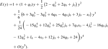
E(y). Also using the improved parameterization y = z/(1 + z), Rezaei et al. (2020) reconstructed the E(z) as a function of y-redshift. The form of the function E(z) can be described as follows:
 (9)
(9)
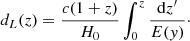
The corresponding luminosity distance can be obtained by using follow formula:
 (10)
(10)
Padé polynomials. The Padé polynomials (Steven & Harold 1992) was built up from the standard Taylor definition and can be used to lower divergences at z≥ 1. It often gives a better approximation for the function than truncating its Taylor series, and it may still work where the Taylar series does not converge (Wei et al. 2014). Due to its excellent convergence properties, the Padé polynomials have been considered at high redshifts in cosmography (Gruber & Luongo 2014; Wei et al. 2014; Demianski et al. 2017; Capozziello et al. 2018b, 2020). The Taylor expansion of a generic function f(z) can be described by a given function 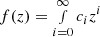 , where ci = fi(0)/i!, which is approximated by means of a (n, m) Padé approximation by the radio polynomial (Capozziello et al. 2020)
 (11)
(11)
there are a total (n + m + 1) number of independent coefficients. In the numerator, we have n + 1 independent coefficients, whereas in the denominator there is m. Since, by construction, b0 = 1 is required, we have
 (12)
(12)
The coefficients bi in Eq. (11) were thus determined by solving the follow homogeneous system of linear equations (Litvinov 1993):
 (13)
(13)
which is valid for k = 1, …, m. All coefficients ai in Eq. (11) can be computed using the formula
 (14)
(14)
In terms of the investigations of Capozziello et al. (2020) on the Padé polynomials, we finally chose to use the Padé(2, 1) approximation and Padé(2, 2) approximation to represent the third-order polynomials and the fourth-order polynomials, respectively. More detailed information about the selections of the specific polynomials can be found in Capozziello et al. (2020). We subsequently provide the corresponding luminosity distances (Capozziello et al. 2020):
(1) Padé(2, 1):
![Mathematical equation: $$ \begin{aligned} d_{L}(z) = \frac{c}{H_{0}}\left[\frac{z(6(-1+q_{0})+(-5-2j_{0}+q_{0}(8+3q_{0}))z)}{-2(3+z+j_{0}z)+2q_{0}(3+z+3q_{0}z)}\right] \cdot \end{aligned} $$](/articles/aa/full_html/2022/05/aa42162-21/aa42162-21-eq16.gif) (15)
(15)
(2) Padé(2, 2):
![Mathematical equation: $$ \begin{aligned} d_{\mathrm{{L}}}(z) =\,&\frac{c}{H_0}\Bigg [6z(10 + 9 z - 6 q_0^3 z + s_0 z - 2 q_0^2 (3 + 7 z) \nonumber \\&- q_0 (16 + 19 z) + j_0 (4 + (9 + 6 q_0) z))\Big /(60 + 24 z \nonumber \\&+ 6 s_0 z - 2 z^2 + 4 j_0^2 z^2 - 9 q_0^4 z^2 - 3 s_0 z^2 \nonumber \\&+ 6 q_0^3 z (-9 + 4 z) + q_0^2 (-36 - 114 z + 19 z^2) \nonumber \\&+ j_0 (24 + 6 (7 + 8 q_0) z + (-7 - 23 q_0 + 6 q_0^2) z^2) \nonumber \\&+ q_0 (-96 - 36 z + (4 + 3 s_0) z^2))\Bigg ]. \end{aligned} $$](/articles/aa/full_html/2022/05/aa42162-21/aa42162-21-eq17.gif) (16)
(16)
log(1 + z). The logarithmic polynomials, log(1 + z), were recently proposed by Risaliti & Lusso (2019) and then adopted to test the flat ΛCDM tension (Lusso et al. 2019; Yang et al. 2020). The new form of the relation between the luminosity distance and the redshift should be written as
![Mathematical equation: $$ \begin{aligned} d_{\mathrm{{L}}}(z) =& k\ \ln (10)\frac{c}{H_{0}}\times \Bigg [\log (1+z)+a_{2}\log ^{2}(1+z) \nonumber \\& + a_{3}\log ^{3}(1+z)+a_{4}\log ^{4}(1+z)\Bigg ] + \textit{O}[\log ^{5}(1+z)]; \nonumber \\ \end{aligned} $$](/articles/aa/full_html/2022/05/aa42162-21/aa42162-21-eq18.gif) (17)
(17)
here, k, a2, a3, and a4 are free parameters.
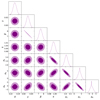 |
Fig. 2. Confidence contours (1σ and 2σ) for the parameters space (δ, γ, β, k, a2, a3, and a4) from the SN-Q sample utilizing the log(1 + z) method. |
log(1 + z) + kij. According to the previous logarithmic polynomials, Bargiacchi et al. (2021) modified the expression of the luminosity distance to make cosmograpgic coefficients with no covariance. They named this method orthogonalized logarithmic polynomials. The modified expression of the luminosity distance is
![Mathematical equation: $$ \begin{aligned} d_{\mathrm{{L}}}(z) =&k\ln (10)\frac{c}{H_{0}}\times \Bigg \{\log (1+z)+a_{2}\log ^{2}(1+z) \nonumber \\& + a_{3}\left[k_{32}\log ^{2}(1+z)+\log ^{3}(1+z)\right]\nonumber \\& + a_{4}\left[k_{42}\log ^{2}(1+z)+k_{43}\log ^{3}(1+z)+\log ^{4}(1+z)\right]\Bigg \} \nonumber \\& + \textit{O}\left[\log ^{5}(1+z)\right], \nonumber \\ \end{aligned} $$](/articles/aa/full_html/2022/05/aa42162-21/aa42162-21-eq19.gif) (18)
(18)
where the coefficients kij are not free parameters and they are associated with our used data set. They were determined through the procedure described in Appendix A of Bargiacchi et al. (2021).
3.2. Statistical analysis and selection criteria
Using the luminosity distance derived from the different cosmographic techniques, we can obtain the corresponding theoretical distance modulus
 (19)
(19)
The best fitting values of the free parameters are achieved by minimizing the value of χ2,
 (20)
(20)
where σi(zi) represents the observational uncertainties of the distance modulus and Pi represents the free parameters to be fitted. For the Pantheon sample, the parameter σi only includes the statistical error. In the GRBs sample, the parameter σi not only contains statistical errors but also takes the intrinsic dispersion σint of the L0–tb correlation into account. For the combination of different datasets, the corresponding  is equal to the sum of χ2 of each dataset. Using the combination of SNe Ia and GRBs as an example, the
  is
is
 (21)
(21)
The likelihood analysis was performed employing a Bayesian Monte Carlo Markov chain (MCMC; Foreman-Mackey et al. 2013) method with the emcee2 package. We used the getdist package (Lewis 2019) to plot the MCMC samples.
 |
Fig. 3. 3D confidence ellipsoid (1σ, 2σ, and 3σ) for the parameters space (a2, a3, and a4) and the corresponding 2D projections on panels a2 − a3, a2 − a4, and a3 − a4 from the SN-Q sample using the log(1 + z) method. The solid orange line shows the relation between two and three parameters in the log(1 + z) model. In 2D projections, red and black points correspond to Ωm = 0.30 and Ωm = 0.40, respectively. In the 3D confidence ellipsoid, the purple point corresponds to Ωm = 0.30. |
Out of necessity, we briefly introduce the model comparison methods used. We note that AIC and BIC are the last set of techniques that can be employed for model comparison based on information theory, and they are widely used in cosmological model comparisons; AIC and BIC are defined by Schwarz (1978) and Akaike (1974), respectively. The corresponding definitions read as follows:
 (22)
(22)
 (23)
(23)
where n is the number of free parameters, N is the total number of data points, and  is the value of χ2 calculated with the best fitting parameters. The model that has lower values of AIC and BIC will be the suitable model for the employed data set. Moreover, we also calculated the differences between ΔAIC and ΔBIC with respect to the corresponding flat ΛCDM values to measure the amount of information lost by adding extra parameters in the statistical fitting. Negative values of ΔAIC and ΔBIC suggest that the model under investigation performs better than the reference model. For positive values of ΔAIC and ΔBIC, we adopt the judgment criteria of the literature (Capozziello et al. 2020):
– ΔAIC(BIC) ∈ [0, 2] indicates weak evidence in favor of the reference model, leaving the question on which model is the most suitable open;
– ΔAIC(BIC) ∈ (2, 6] indicates mild evidence against the given model with respect to the reference paradigm; and
– ΔAIC(BIC) > 6 indicates strong evidence against the given model, which should be rejected.
4. Potential deviation from ΛCDM from quasar data
Risaliti & Lusso (2019) found a 4σ deviation from ΛCDM via the Hubble diagram of SNe Ia and 1598 quasars. Then Lusso et al. (2019) confirmed the tension between the ΛCDM model and the best cosmographic parameters at 4σ with SNe Ia from the Pantheon sample and quasars, and at > 4σ with SNe Ia, quasars, and GRBs. These two works both used a calibrated quasar relation between the UV and X-ray luminosity which can be parameterized as (Avni & Tananbaum 1986)
 (24)
(24)
where LX is the rest-frame monochromatic luminosity at 2 keV and LUV is the luminosity at 2500 Å. We note that γ and β are fixed (Risaliti & Lusso 2019), and then they were used for the cosmological constraints. The details on the calibration of quasar relation between the UV and X-ray luminosity are provided in Risaliti & Lusso (2019). In this section, we fit the quasar relation and cosmographic parameters simultaneously.
Utilizing Eq. (24), we derived the theorietical X-ray flux (Hu et al. 2020; Khadka & Ratra 2020b):
![Mathematical equation: $$ \begin{aligned} \phi ([F_{\mathrm{{UV}}}]_{i},d_{L}[z_{i}]) =&\log (F_{X}) \nonumber \\ =&\gamma (\log {F_{\mathrm{{UV}}}}) +(\gamma -1)\log {4\pi } \nonumber \\& + 2(\gamma -1)\log {d_{L}} + \beta . \end{aligned} $$](/articles/aa/full_html/2022/05/aa42162-21/aa42162-21-eq29.gif) (25)
(25)
Here, Fx and FUV represent the X-ray and UV flux, respectively. For the Padé(2,1) approximation and logarithmic polynomials, the corresponding luminosity distances dL were calculated by utilizing Eqs. (15) and (17), respectively. For the quasar sample, the best fitting values of our used parameters can be obtained by minimizing the corresponding  ,
,
![Mathematical equation: $$ \begin{aligned} \chi ^{2}_{Q} \ =\ \sum _{i=1}^{1598}\left(\frac{(\log (F_{X})_{i}-\phi ([F_{\mathrm{{UV}}}]_{i},d_{L}[z_{i}]))^{2}}{s_{i}^{2}} + \ln \left(2\pi s_{i}^{2}\right)\right), \end{aligned} $$](/articles/aa/full_html/2022/05/aa42162-21/aa42162-21-eq31.gif) (26)
(26)
where the variance  consists of the global intrinsic scatter δ and the measurement error σi in (FX)i, that is
  . Compared to δ and
  , the error of (FUV)i is negligible. The function ϕ corresponds to the theoretical X-ray flux obtained by Eq. (25). Combining Eqs. (17), (25), and (26), we can obtain the fitting results, that is δ = 0.23 ± 0.01, γ = 0.63 ± 0.01, β = 7.42 ± 0.32, k = 0.99 ± 0.01, a2 = 3.08 ± 0.17, a3 = 3.70 ± 1.10, and
  . The corresponding confidence contours are shown in Fig. 2. In Fig. 3, we plotted the 3D confidence ellipsoid for parameters space (a2, a3, and a4) and the corresponding 2D projections on panels a2 − a3, a2 − a4, and a3 − a4. The solid orange lines show the relation between parameters a2, a3, and a4. It is easy to find that the constrained results of the 2D projections are consistent with the flat ΛCDM model within the 2σ level. The results of the 3D confidence ellipsoid are consistent with the flat ΛCDM model within the 3σ level. Through analyzing Figs. 2 and 3, we confirm that considering correlation parameters δ, γ, and β as free parameters, the 4σ tension between the ΛCDM model and the best cosmographic parameters from the SN-Q sample reduce to 3σ.
While using the Padé(2,1) approximation, we checked the influence of the quasar relation on the cosmological constraints. We first provide the constraints considering a free quasar relation. Then combining that with the following two special cases, the effect of the slope parameter γ is studied. One case is the fitting parameters q0 and j0 in the case of fixed parameters δ, γ, and β. The other is to refit q0 and j0 by changing the setting of the fixed parameter γ within a 1σ error (0.005). The fixed parameters δ, γ, and β are given in terms of the best fitting results from 1598 quasars in a flat ΛCDM model. By substituting Eqs. (25) into (26), and replacing dL with Eq. (6), we obtained the best fits, that is  , δ = 0.23 ± 0.01, γ = 0.62 ± 0.01, and β = 7.60 ± 0.28. This result is consistent with previous research within a 1σ error (Lusso & Risaliti 2016; Melia 2019; Salvestrini et al. 2019; Khadka & Ratra 2020a, 2022; Liu et al. 2020; Wei & Melia 2020). Here, it is worth noting that the 1σ errors of the γ best fit from previous research are both larger than 0.01. Figure 4 shows the fitting results with a free quasar relation. The best fits are δ = 0.23 ± 0.01, γ = 0.64 ± 0.01,
  , q0 = −0.67 ± 0.04, and
  . This result is in line with the previous results obtained by the logarithmic polynomials. The corresponding q0 − j0 projection is also plotted in Fig. 5 as a gray contour. In addition, we also show the confidence contours of the other two special cases. (1) When we chose δ = 0.23, γ = 0.62, and β = 7.60 (best fits from 1598 quasars in a flat ΛCDM model), the results are q0 = −0.82 ± 0.05 and
  , which is represented by the red contours in Fig. 5. There exists more than a 4σ tension with the flat ΛCDM. (2) In only changing γ = 0.625, the new result is q0 = −0.58 ± 0.03 and
  which is described by the blue contours of Fig. 5. We find that the γ value changes from 0.62 to 0.625 (within a 1σ error of 0.01), and the 4σ tension disappears. This result is consistent with the ΛCDM model within a 1σ level. We find that the quasar relation can obviously affect the cosmographic constraint, especially the slope parameter γ.
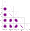 |
Fig. 4. Confidence contours (1σ and 2σ) for the parameters space (δ, γ, β, q0, and j0) from the SN-Q sample using the Padé(2,1) method. |
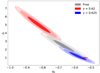 |
Fig. 5. Confidence contours (1σ, 2σ, and 3σ) for the parameters space (q0 and j0) from the SN-Q sample utilizing the Padé(2,1) method. The red point represents (−0.54, 1) the value given by the Planck 2018 results (Planck Collaboration VII 2020). |
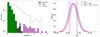 |
Fig. 6. Fundamental information about the used data sets. Left panel: redshift distribution of SNe Ia, GRBs, and quasars. Right panel: constrained results of Ωm from different combinations of SNe Ia, GRBs, and quasars in the spatially flat ΛCDM model. |
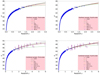 |
Fig. 7. Hubble diagram of SNe Ia and GRBs. The upper two panels and the lower two panels use the Pantheon sample and the combined sample, respectively. The expansion order of the right two panels and the left two panels is different. The former is the third order and the latter is the fourth order. Blue points are SNe Ia from the Pantheon sample. Purple points are 31 LGRBs constructed by Wang et al. (2022). |
Best fitting results obtained from the Pantheon sample using different cosmographic techniques.
Best fitting results obtained from the combined sample using different cosmographic techniques.
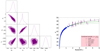 |
Fig. 8. Comparison between different expansion orders using the y-redshift method. Right panel: confidence contours (1σ and 2σ) for the parameters space (q0, j0, s0, and l0) from the combined sample. Blue points are SNe Ia from the Pantheon sample. Purple points are 31 LGRBs constructed by Wang et al. (2022). |
5. Results
Firstly, we performed an analysis of the used samples, including the redshift distribution and the constraints on Ωm in the spatially flat ΛCDM model, as shown in Fig. 6. From the redshift distribution, we found that SNe Ia are mainly distributed in low redshift (z < 1), and GRBs and quasars are mainly distributed in high redshift (z > 1). The best fits of Ωm are all near 0.29 with a 1σ error of 0.01. This result will be used in subsequent comparisons. Below, we show the main results.
A comparison with different cosmographic methods as another main work also yields many meaningful results. We plotted the Hubble diagram of SNe Ia and GRBs, as well as the corresponding theoretical lines with different methods or different expansion orders, as shown in Fig. 7. The upper two panels and the lower two panels use the Pantheon sample and a combination of the Pantheon sample and 31 LGRBs, respectively. Expansion orders of the right two panels and the left two panels are the third order and the fourth order, respectively. By analyzing Fig. 7, we found that as the expansion order increases, the difference between the prediction lines of different methods becomes blurred. However, the results of the y-refshift method are obviously different from other methods. This is one of the reasons why we studied the y-redshift with different expansion orders separately. The corresponding best fitting results and statistical information ( , AIC, BIC, ΔAIC, and ΔBIC) of the Pantheon sample and the combined sample are listed in Tables 1 and 2, respectively.
In Table 1, among the results of the third-order expansion, the smallest values for ΔAIC and ΔBIC were all obtained by the Padé(2,1) method, that is ΔAIC = 0.83 and ΔBIC = 1.85. Also, ΔAIC and ΔBIC of the z-redshift method are close to the values of the former. The ones of the y-redshift and the E(y) methods are ΔAIC = 72.48 and ΔBIC = 73.50, and ΔAIC = 8.29 and ΔBIC = 9.31, respectively, which are both larger than 6. The latter values are significantly better than the former. From the results of the fourth-order expansion, the smallest values for ΔAIC and ΔBIC are 1.63 and 3.67, which are given by the z-redshift method. Utilizing the Padé(2,2) method, we found that ΔAIC = 7.89 and ΔBIC = 10.02, which are larger than what was found for the other methods. The results for the y-redshift and E(y) methods are similar. Combining the results of third-order expansion with the results of firth-order expansion, the minimum values of ΔAIC and ΔBIC from Table 1 are ΔAIC = 0.83 and ΔBIC = 1.85, which were obtained by the Padé(2,1) method. Through analyzing statistical information in Table 1, it is easy to find that, except for the y-redshift and E(y) methods, the values of ΔAIC and ΔBIC increase with the expansion order. In comparison to other methods, the influence of the expansion order on the results for the y-redshift method is more obvious. For the Pantheon sample (low redshift case), the third-order expansion of y-redshift and E(y) methods and Padé(2,2) can be rule out based on the values for ΔAIC and ΔBIC.
In Table 2, one can notice that there is no convergent result from the combined sample using the third-order expansion of the z-redshift method. From the third-order results, the values for ΔAIC and ΔBIC obtained by the Padé(2,1), log(1 + z), and log(1 + z)+kij methods are very close, and they are all less than 2. For the Padé(2,1) method, the values for ΔAIC and ΔBIC are 0.23 and 1.27, respectively. For the log(1 + z) and log(1 + z)+kij methods, the corresponding results are ΔAIC = −0.15 and ΔBIC = 1.92, and ΔAIC = −0.15 and ΔBIC = 1.91, respectively. The results obtained from the y-redshift and E(y) methods are both larger than 6. For the fourth-order case, the minimum values, ΔAIC = 0.49 and ΔBIC = 2.56, were obtained by the Padé(2,2) method. The results of the y-redshift and E(y) methods are still greater than 6 and those for the former are worse. Minimum values of ΔAIC and ΔBIC in Table 2 are also given by the Padé(2,1) method. Looking through the results of Table 2, we found that the main conclusions obtained from the Pantheon sample are both confirmed by employing the combined sample including the Pantheon sample and 31 LGRBs (high-redshift case). In the case of high redshift, the fourth-order expansions of y-redshift and E(y) are also excluded.
And we also found some interesting results. There is no convergent result using the third-order expansion of the z-redshift method, but the fourth-order expansion can be used to obtain a good result. The Padé(2,2) method, which is ruled out in the case of low redshift (Pantheon sample), also has a good result. It demonstrates that it is important to choose the suitable expansion method and order based on the sample used. In Table 2, we present the constraints of the fifth-order expansion and the corresponding Hubble diagram from the combined sample using the y-redshift method, as shown in the left panel and the right panel of Fig. 8, respectively. The best fits are  ,
,  , s0 = 379.04 ± 94.00, and l0 = −4170 ± 1100. The values for ΔAIC and ΔBIC are equal to 5.85 and 8.96, which are smaller than what was obtained by the third-order expansion and fourth-order expansion. To understand the influence of the expansion order on the results more intuitively, the third-order and the fourth-order expansions are also plotted in the right panel of Fig. 8. We find that the theoretical line of higher order is closer to that of the flat ΛCDM model. At the same time, from the results of the y-redshift method in Table 2, we confirm that the values for ΔAIC and ΔBIC decrease with the expansion order increase.
All confidence contours corresponding to Tables 1 and 2 are shown in Figs. A.1–A.4. Figures A.1 and A.2 were obtained by utilizing the Pantheon sample for the third order and the fourth order, respectively. Figures A.3 and A.4 are similar to Figs. A.1 and A.2, except that the combined sample is used for the former. In order to better display the results of comparison, we drew the consequences of the same parameters in a graph. The results of y-redshift are not tight and deviate significantly from other results. So we plotted the y-redshift results in a single graph.
6. Conclusions and discussion
In this paper, we first investigate the effect of the quasar relation between the UV and X-ray luminosities on the cosmographic constraints using the logarithmic polynomials and Padé(2,1) methods. Then based on the Pantheon sample and 31 LGRBs, we critically compare six kinds of cosmographic methods, that is z-redshift, y-redshift, E(y), log(1 + z), log(1 + z)+kij, and Padé polynomials. By investigating the effect of the quasar relation on the cosmographic constraint, we were able to find that the quasar relation can obviously affect the cosmographic constraint, especially the slope parameter γ. The change in the γ value by 0.005 makes the 4σ tension disappear. And until now, the best fits of the calibrated γ have been in the range (0.612, 0.648), which was obtained from the latest quasar sample using different calibrated methods (Risaliti & Lusso 2019; Wei & Melia 2020; Li et al. 2021; Zheng et al. 2021). In terms of our study, the γ value changes from 0.612 to 0.648, and the tension changes significantly. This indicates that the 4σ or 3σ tension between the ΛCDM model and the best cosmographic parameters from the SN-Q sample may be uncertain. In order to better constrain the cosmographic parameters, we need more precise data of quasars to yield a tighter quasar relation. A next-generation X-ray, such as eROSITA (Lusso 2020), will provide us more copious and precise data for quasars which could help us solve this puzzle.
Our other main interest is to compare different cosmographic techniques by combining new high-redshift data. We adopted the AIC and BIC selection criteria as tools for inferring the statistical significance of a given scenario with respect to the ΛCDM model. The corresponding results are shown in Figs. 7, 8 and Tables 1, 2. By analyzing the theoretical lines produced by different methods and different orders, we found that increasing the order makes the theoretical predictions obtained by different methods closer to the predictions of the ΛCDM model with Ωm = 0.29. Among them, the increase in the order has the most obvious influence on the y-redshift method. This can also be found from the changes in ΔAIC and ΔBIC. For the Pantheon sample, Padé(2,1) turns out to be the best-performing approximation in the third- and fourth-order expansions. The third-order expansions of the y-redshift and E(y) methods can be ruled out. For the combined sample, the Padé(2,1) approximation still performs well. The third- and fourth-order expansions of the y-redshift and E(y) methods are both excluded. The E(y) method is better than the y-redshift method. On the contrary, the log(1 + z) and log(1 + z)+kij methods have good performance in these two expansion orders. Combining all of the results, we found that the Padé(2,1) method is suitable for low and high redshift cases. The Padé(2,2) method performs well in high redshift situations. The performance of the E(y) method is better than that of the y-redshift method. The log(1 + z) and log(1 + z)+kij methods are better than the z-redshift, y-redshift, and E(y) methods, but worse than Padé approximations. Except for the y-redshift and E(y) methods, the values of ΔAIC and ΔBIC increase with the expansion order. But the constraints of the y-redshift and E(y) methods may be problematic, that is, the high-order coefficients are abnormal. To minimize risk, one might only constrain the first two parameters (q0 and j0), and the other parameters could be marginalized in a large range (Zhang et al. 2017; Wang et al. 2022).
Acknowledgments
We thank the anonymous referee for helpful comments. This work was supported by the National Natural Science Foundation of China (grant No. U1831207) and the China Manned Spaced Project (CMS-CSST-2021-A12).
References
- Akaike, H. 1974, IEEE Trans. Autom. Control, 19, 716 [Google Scholar]
- Aviles, A., Bravetti, A., Capozziello, S., & Luongo, O. 2014, Phys. Rev. D, 90, 043531 [NASA ADS] [CrossRef] [Google Scholar]
- Avni, Y., & Tananbaum, H. 1986, ApJ, 305, 83 [Google Scholar]
- Banerjee, A., Ó Colgáin, E., Sasaki, M., Sheikh-Jabbari, M. M., & Yang, T. 2021, Phys. Lett. B, 818, 136366 [NASA ADS] [CrossRef] [Google Scholar]
- Bargiacchi, G., Risaliti, G., Benetti, M., et al. 2021, A&A, 649, A65 [NASA ADS] [CrossRef] [EDP Sciences] [Google Scholar]
- Betoule, M., Kessler, R., Guy, J., et al. 2014, A&A, 568, A22 [NASA ADS] [CrossRef] [EDP Sciences] [Google Scholar]
- Bonilla, A., D’Agostino, R., Nunes, R. C., & de Araujo, J. C. N. 2020, JCAP, 2020, 015 [CrossRef] [Google Scholar]
- Busti, V. C., de la Cruz-Dombriz, Á., Dunsby, P. K. S., & Sáez-Gómez, D. 2015, Phys. Rev. D, 92, 123512 [NASA ADS] [CrossRef] [Google Scholar]
- Cai, R.-G., Guo, Z.-K., Wang, S.-J., Yu, W.-W., & Zhou, Y. 2022, Phys. Rev. D, 105, L021301 [NASA ADS] [CrossRef] [Google Scholar]
- Caldwell, R. R., & Kamionkowski, M. 2004, JCAP, 2004, 009 [NASA ADS] [CrossRef] [Google Scholar]
- Cao, S., Khadka, N., & Ratra, B. 2022, MNRAS, 510, 2928 [NASA ADS] [CrossRef] [Google Scholar]
- Capozziello, S., & Ruchika Sen, A. A. 2019, MNRAS, 484, 4484 [NASA ADS] [CrossRef] [Google Scholar]
- Capozziello, S., Lazkoz, R., & Salzano, V. 2011, Phys. Rev. D, 84, 124601 [NASA ADS] [Google Scholar]
- Capozziello, S., D’Agostino, R., & Luongo, O. 2018a, MNRAS, 476, 3924 [NASA ADS] [CrossRef] [Google Scholar]
- Capozziello, S., D’Agostino, R., & Luongo, O. 2018b, JCAP, 2018, 008 [CrossRef] [Google Scholar]
- Capozziello, S., D’Agostino, R., & Luongo, O. 2019, Int. J. Mod. Phys. D, 28, 1930016 [NASA ADS] [CrossRef] [Google Scholar]
- Capozziello, S., D’Agostino, R., & Luongo, O. 2020, MNRAS, 494, 2576 [NASA ADS] [CrossRef] [Google Scholar]
- Carroll, S. M. 2001, Liv. Rev. Relat., 4, 1 [NASA ADS] [CrossRef] [Google Scholar]
- Cattoën, C., & Visser, M. 2007, Class. Quant. Grav., 24, 5985 [CrossRef] [Google Scholar]
- Chevallier, M., & Polarski, D. 2001, Int. J. Mod. Phys. D, 10, 213 [Google Scholar]
- Chiba, T., & Nakamura, T. 1998, in 19th Texas Symposium on Relativistic Astrophysics and Cosmology, eds. J. Paul, T. Montmerle, & E. Aubourg, 276 [Google Scholar]
- Conley, A., Guy, J., Sullivan, M., et al. 2011, ApJS, 192, 1 [Google Scholar]
- Contreras, C., Hamuy, M., Phillips, M. M., et al. 2010, AJ, 139, 519 [Google Scholar]
- D’Agostino, R., & Nunes, R. C. 2019, Phys. Rev. D, 100, 044041 [CrossRef] [Google Scholar]
- Dai, Z. G., & Lu, T. 1998, A&A, 333, L87 [NASA ADS] [Google Scholar]
- Demianski, M., Piedipalumbo, E., Sawant, D., & Amati, L. 2017, A&A, 598, A113 [NASA ADS] [CrossRef] [EDP Sciences] [Google Scholar]
- Demianski, M., Piedipalumbo, E., Sawant, D., & Amati, L. 2021, MNRAS, 506, 903 [NASA ADS] [CrossRef] [Google Scholar]
- Dunsby, P. K. S., & Luongo, O. 2016, Int. J. Geom. Meth. Mod. Phys., 13, 1630002 [NASA ADS] [CrossRef] [Google Scholar]
- Folatelli, G., Phillips, M. M., Burns, C. R., et al. 2010, AJ, 139, 120 [Google Scholar]
- Foreman-Mackey, D., Hogg, D. W., Lang, D., & Goodman, J. 2013, PASP, 125, 306 [Google Scholar]
- Frieman, J. A., Bassett, B., Becker, A., et al. 2008, AJ, 135, 338 [Google Scholar]
- Graur, O., Rodney, S. A., Maoz, D., et al. 2014, ApJ, 783, 28 [NASA ADS] [CrossRef] [Google Scholar]
- Green, P. J., Aldcroft, T. L., Richards, G. T., et al. 2009, ApJ, 690, 644 [Google Scholar]
- Gruber, C., & Luongo, O. 2014, Phys. Rev. D, 89, 103506 [NASA ADS] [CrossRef] [Google Scholar]
- Hicken, M., Challis, P., Jha, S., et al. 2009a, ApJ, 700, 331 [Google Scholar]
- Hicken, M., Wood-Vasey, W. M., Blondin, S., et al. 2009b, ApJ, 700, 1097 [Google Scholar]
- Hicken, M., Challis, P., Kirshner, R. P., et al. 2012, ApJS, 200, 12 [Google Scholar]
- Hu, J. P., Wang, Y. Y., & Wang, F. Y. 2020, A&A, 643, A93 [EDP Sciences] [Google Scholar]
- Hu, J. P., Wang, F. Y., & Dai, Z. G. 2021, MNRAS, 507, 730 [NASA ADS] [CrossRef] [Google Scholar]
- Jha, S., Kirshner, R. P., Challis, P., et al. 2006, AJ, 131, 527 [Google Scholar]
- Jin, C., Ward, M., & Done, C. 2012, MNRAS, 422, 3268 [Google Scholar]
- Just, D. W., Brandt, W. N., Shemmer, O., et al. 2007, ApJ, 665, 1004 [Google Scholar]
- Kessler, R., Becker, A. C., Cinabro, D., et al. 2009, ApJS, 185, 32 [Google Scholar]
- Khadka, N., & Ratra, B. 2020a, MNRAS, 497, 263 [Google Scholar]
- Khadka, N., & Ratra, B. 2020b, MNRAS, 492, 4456 [NASA ADS] [CrossRef] [Google Scholar]
- Khadka, N., & Ratra, B. 2022, MNRAS, 510, 2753 [NASA ADS] [CrossRef] [Google Scholar]
- Lewis, A. 2019, ArXiv e-prints [arXiv:1910.13970] [Google Scholar]
- Li, E.-K., Du, M., & Xu, L. 2020, MNRAS, 491, 4960 [NASA ADS] [CrossRef] [Google Scholar]
- Li, X., Keeley, R. E., Shafieloo, A., et al. 2021, MNRAS, 507, 919 [NASA ADS] [CrossRef] [Google Scholar]
- Linder, E. V. 2003, Phys. Rev. Lett., 90, 091301 [Google Scholar]
- Litvinov, G. 1993, Russ. J. Math. Phys., 36, 313 [Google Scholar]
- Liu, T., Cao, S., Biesiada, M., et al. 2020, ApJ, 899, 71 [NASA ADS] [CrossRef] [Google Scholar]
- Lusso, E. 2020, Front. Astron. Space Sci., 7, 8 [NASA ADS] [CrossRef] [Google Scholar]
- Lusso, E., & Risaliti, G. 2016, ApJ, 819, 154 [Google Scholar]
- Lusso, E., Piedipalumbo, E., Risaliti, G., et al. 2019, A&A, 628, L4 [NASA ADS] [CrossRef] [EDP Sciences] [Google Scholar]
- Melia, F. 2019, MNRAS, 489, 517 [NASA ADS] [CrossRef] [Google Scholar]
- Planck Collaboration VII. 2020, A&A, 641, A7 [NASA ADS] [CrossRef] [EDP Sciences] [Google Scholar]
- Rest, A., Scolnic, D., Foley, R. J., et al. 2014, ApJ, 795, 44 [Google Scholar]
- Rezaei, M., Pour-Ojaghi, S., & Malekjani, M. 2020, ApJ, 900, 70 [NASA ADS] [CrossRef] [Google Scholar]
- Riess, A. G., Kirshner, R. P., Schmidt, B. P., et al. 1999, AJ, 117, 707 [Google Scholar]
- Riess, A. G., Strolger, L.-G., Tonry, J., et al. 2004, ApJ, 607, 665 [NASA ADS] [CrossRef] [Google Scholar]
- Riess, A. G., Strolger, L.-G., Casertano, S., et al. 2007, ApJ, 659, 98 [NASA ADS] [CrossRef] [Google Scholar]
- Riess, A. G., Rodney, S. A., Scolnic, D. M., et al. 2018, ApJ, 853, 126 [NASA ADS] [CrossRef] [Google Scholar]
- Risaliti, G., & Lusso, E. 2015, ApJ, 815, 33 [NASA ADS] [CrossRef] [Google Scholar]
- Risaliti, G., & Lusso, E. 2019, Nat. Astron., 3, 272 [Google Scholar]
- Rodney, S. A., Riess, A. G., Strolger, L.-G., et al. 2014, AJ, 148, 13 [Google Scholar]
- Sako, M., Bassett, B., Becker, A. C., et al. 2018, PASP, 130, 064002 [NASA ADS] [CrossRef] [Google Scholar]
- Salvestrini, F., Risaliti, G., Bisogni, S., Lusso, E., & Vignali, C. 2019, A&A, 631, A120 [NASA ADS] [CrossRef] [EDP Sciences] [Google Scholar]
- Schwarz, G. 1978, Ann. Stat., 6, 461 [Google Scholar]
- Scolnic, D., Rest, A., Riess, A., et al. 2014, ApJ, 795, 45 [Google Scholar]
- Scolnic, D. M., Jones, D. O., Rest, A., et al. 2018, ApJ, 859, 101 [NASA ADS] [CrossRef] [Google Scholar]
- Shafieloo, A. 2012, JCAP, 2012, 002 [NASA ADS] [CrossRef] [Google Scholar]
- Speri, L., Tamanini, N., Caldwell, R. R., Gair, J. R., & Wang, B. 2021, Phys. Rev. D, 103, 083526 [NASA ADS] [CrossRef] [Google Scholar]
- Steffen, A. T., Strateva, I., Brandt, W. N., et al. 2006, AJ, 131, 2826 [Google Scholar]
- Steven, G. K., & Harold, R. P. 1992, Birkhuser Adv. Texts, 39, 373 [Google Scholar]
- Strateva, I. V., Brandt, W. N., Schneider, D. P., Vanden Berk, D. G., & Vignali, C. 2005, AJ, 130, 387 [Google Scholar]
- Stritzinger, M. D., Phillips, M. M., Boldt, L. N., et al. 2011, AJ, 142, 156 [Google Scholar]
- Sullivan, M., Guy, J., Conley, A., et al. 2011, ApJ, 737, 102 [NASA ADS] [CrossRef] [Google Scholar]
- Suzuki, N., Rubin, D., Lidman, C., et al. 2012, ApJ, 746, 85 [NASA ADS] [CrossRef] [Google Scholar]
- Tripp, R. 1998, A&A, 331, 815 [NASA ADS] [Google Scholar]
- Vignali, C., Brandt, W. N., & Schneider, D. P. 2003, AJ, 125, 433 [Google Scholar]
- Visser, M. 2004, Class. Quant. Grav., 21, 2603 [NASA ADS] [CrossRef] [Google Scholar]
- Visser, M. 2015, Class. Quant. Grav., 32, 135007 [NASA ADS] [CrossRef] [Google Scholar]
- Vitagliano, V., Xia, J.-Q., Liberati, S., & Viel, M. 2010, JCAP, 2010, 005 [CrossRef] [Google Scholar]
- Wang, J. S., & Wang, F. Y. 2014, MNRAS, 443, 1680 [NASA ADS] [CrossRef] [Google Scholar]
- Wang, F. Y., Dai, Z. G., & Qi, S. 2009, A&A, 507, 53 [NASA ADS] [CrossRef] [EDP Sciences] [Google Scholar]
- Wang, F. Y., Dai, Z. G., & Liang, E. W. 2015, New Astron. Rev., 67, 1 [CrossRef] [Google Scholar]
- Wang, J. S., Wang, F. Y., Cheng, K. S., & Dai, Z. G. 2016, A&A, 585, A68 [NASA ADS] [CrossRef] [EDP Sciences] [Google Scholar]
- Wang, F. Y., Hu, J. P., Zhang, G. Q., & Dai, Z. G. 2022, ApJ, 924, 97 [NASA ADS] [CrossRef] [Google Scholar]
- Wei, J.-J., & Melia, F. 2020, ApJ, 888, 99 [NASA ADS] [CrossRef] [Google Scholar]
- Wei, J.-J., & Wu, X.-F. 2017, Int. J. Mod. Phys. D, 26, 1730002 [NASA ADS] [CrossRef] [Google Scholar]
- Wei, H., Yan, X.-P., & Zhou, Y.-N. 2014, JCAP, 2014, 045 [CrossRef] [Google Scholar]
- Weinberg, S. 1972, Gravitation and Cosmology: Principles and Applications of the General Theory of Relativity (New York: Wiley) [Google Scholar]
- Yang, T., Banerjee, A., & Ó Colgáin, E. 2020, Phys. Rev. D, 102, 1730002 [Google Scholar]
- Yin, Z.-Y., & Wei, H. 2019, Eur. Phys. J. C, 79, 698 [NASA ADS] [CrossRef] [Google Scholar]
- Young, M., Elvis, M., & Risaliti, G. 2009, ApJS, 183, 17 [NASA ADS] [CrossRef] [Google Scholar]
- Young, M., Elvis, M., & Risaliti, G. 2010, ApJ, 708, 1388 [Google Scholar]
- Yu, H., Ratra, B., & Wang, F.-Y. 2018, ApJ, 856, 3 [NASA ADS] [CrossRef] [Google Scholar]
- Zamora Munõz, C., & Escamilla-Rivera, C. 2020, JCAP, 2020, 007 [CrossRef] [Google Scholar]
- Zhang, B., & Mészáros, P. 2001, ApJ, 552, L35 [CrossRef] [Google Scholar]
- Zhang, M.-J., Li, H., & Xia, J.-Q. 2017, Eur. Phys. J. C, 77, 434 [NASA ADS] [CrossRef] [Google Scholar]
- Zhao, D., & Xia, J.-Q. 2021, Eur. Phys. J. C, 81, 948 [NASA ADS] [CrossRef] [Google Scholar]
- Zheng, X., Cao, S., Biesiada, M., et al. 2021, Sci. China Phys. Mech. Astron., 64, 259511 [NASA ADS] [CrossRef] [Google Scholar]
Appendix A: 1σ and 2σ contours in the 2D parameter space utilizing different expansion orders and datasets
 |
Fig. A.1. Confidence contours (1σ and 2σ) for the cosmographic parameters space using the Pantheon sample and the third-order expansion. |
 |
Fig. A.2. Confidence contours (1σ and 2σ) for the cosmographic parameters space using the Pantheon sample and the fourth-order expansion. |
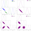 |
Fig. A.3. Confidence contours (1σ and 2σ) for the cosmographic parameters space using the combined sample and the third-order expansion. |
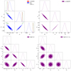 |
Fig. A.4. Confidence contours (1σ and 2σ) for the cosmographic parameters space using the combined sample and the fourth-order expansion. |
All Tables
Best fitting results obtained from the Pantheon sample using different cosmographic techniques.
Best fitting results obtained from the combined sample using different cosmographic techniques.
All Figures
|
Fig. 1. Hubble diagram of SNe Ia, GRBs, and quasars. The picture includes 1048 SNe Ia of the Pantheon sample, 31 LGRBs, and 1598 quasars. The black solid line is a flat ΛCDM model with Ωm = 0.3 and Hubble constant H0 = 70 km s−1 Mpc−1. Distance moduli and corresponding errors are provided by Risaliti & Lusso (2019) which were calculated by the calibrated UV and X-ray correlation using the low-redshift SNe Ia. |
| In the text | |
|
Fig. 2. Confidence contours (1σ and 2σ) for the parameters space (δ, γ, β, k, a2, a3, and a4) from the SN-Q sample utilizing the log(1 + z) method. |
| In the text | |
|
Fig. 3. 3D confidence ellipsoid (1σ, 2σ, and 3σ) for the parameters space (a2, a3, and a4) and the corresponding 2D projections on panels a2 − a3, a2 − a4, and a3 − a4 from the SN-Q sample using the log(1 + z) method. The solid orange line shows the relation between two and three parameters in the log(1 + z) model. In 2D projections, red and black points correspond to Ωm = 0.30 and Ωm = 0.40, respectively. In the 3D confidence ellipsoid, the purple point corresponds to Ωm = 0.30. |
| In the text | |
|
Fig. 4. Confidence contours (1σ and 2σ) for the parameters space (δ, γ, β, q0, and j0) from the SN-Q sample using the Padé(2,1) method. |
| In the text | |
|
Fig. 5. Confidence contours (1σ, 2σ, and 3σ) for the parameters space (q0 and j0) from the SN-Q sample utilizing the Padé(2,1) method. The red point represents (−0.54, 1) the value given by the Planck 2018 results (Planck Collaboration VII 2020). |
| In the text | |
|
Fig. 6. Fundamental information about the used data sets. Left panel: redshift distribution of SNe Ia, GRBs, and quasars. Right panel: constrained results of Ωm from different combinations of SNe Ia, GRBs, and quasars in the spatially flat ΛCDM model. |
| In the text | |
|
Fig. 7. Hubble diagram of SNe Ia and GRBs. The upper two panels and the lower two panels use the Pantheon sample and the combined sample, respectively. The expansion order of the right two panels and the left two panels is different. The former is the third order and the latter is the fourth order. Blue points are SNe Ia from the Pantheon sample. Purple points are 31 LGRBs constructed by Wang et al. (2022). |
| In the text | |
|
Fig. 8. Comparison between different expansion orders using the y-redshift method. Right panel: confidence contours (1σ and 2σ) for the parameters space (q0, j0, s0, and l0) from the combined sample. Blue points are SNe Ia from the Pantheon sample. Purple points are 31 LGRBs constructed by Wang et al. (2022). |
| In the text | |
|
Fig. A.1. Confidence contours (1σ and 2σ) for the cosmographic parameters space using the Pantheon sample and the third-order expansion. |
| In the text | |
|
Fig. A.2. Confidence contours (1σ and 2σ) for the cosmographic parameters space using the Pantheon sample and the fourth-order expansion. |
| In the text | |
|
Fig. A.3. Confidence contours (1σ and 2σ) for the cosmographic parameters space using the combined sample and the third-order expansion. |
| In the text | |
|
Fig. A.4. Confidence contours (1σ and 2σ) for the cosmographic parameters space using the combined sample and the fourth-order expansion. |
| In the text | |
Current usage metrics show cumulative count of Article Views (full-text article views including HTML views, PDF and ePub downloads, according to the available data) and Abstracts Views on Vision4Press platform.
Data correspond to usage on the plateform after 2015. The current usage metrics is available 48-96 hours after online publication and is updated daily on week days.
Initial download of the metrics may take a while.