| Issue |
A&A
Volume 661, May 2022
The Early Data Release of eROSITA and Mikhail Pavlinsky ART-XC on the SRG mission
|
|
|---|---|---|
| Article Number | A29 | |
| Number of page(s) | 23 | |
| Section | Stellar atmospheres | |
| DOI | https://doi.org/10.1051/0004-6361/202141617 | |
| Published online | 18 May 2022 | |
First eROSITA study of nearby M dwarfs and the rotation-activity relation in combination with TESS★
1
Institut für Astronomie und Astrophysik, Eberhard-Karls Universität Tübingen,
Sand 1,
72076
Tübingen, Germany
e-mail: This email address is being protected from spambots. You need JavaScript enabled to view it.
2
INAF – Osservatorio Astronomico di Palermo,
Piazza Parlamento 1,
90134
Palermo, Italy
3
Max-Planck-Institut für extraterrestrische Physik,
Giessenbachstr. 1,
85748
Garching, Germany
4
Exzellenzcluster ORIGINS,
Boltzmannstr. 2,
85748
Garching, Germany
Received:
22
June
2021
Accepted:
29
November
2021
Abstract
We present the first results with the ROentgen Survey with an Imaging Telescope Array (eROSITA) on board the Russian Spektrum-Roentgen-Gamma mission, and we combine the new X-ray data with observations with the Transiting Exoplanet Survey Satellite (TESS). We used the SUPERBLINK proper motion catalog of nearby M dwarfs as input sample to search for eROSITA and TESS data. We extracted Gaia DR2 data for the full M dwarf catalog, which comprises ~9000 stars, and we calculated the stellar parameters from empirical relations with optical/IR colors. Then we cross-matched this catalog with the eROSITA Final Equatorial Depth Survey (eFEDS) and the first eROSITA all-sky survey (eRASS1). After a meticulous source identification in which we associated the closest Gaia source with the eROSITA X-ray detections, our sample of M dwarfs is defined by 687 stars with SpT = K5..M7 (673 from eRASS1 and 14 from eFEDS). While for eRASSl we used the data from the source catalog provided by the eROSITA_DE consortium, for the much smaller eFEDS sample, we performed the data extraction, and we analyzed the X-ray spectra and light curves. This unprecedented data base for X-ray emitting M dwarfs allowed us to place a quantitative constraint on the mass dependence of the X-ray luminosity, and to determine the change in the activity level with respect to pre-main-sequence stars. TESS observations are available for 489 of 687 X-ray detected M dwarfs. By applying standard period search methods, we were able to determine the rotation period for 180 X-ray detected M dwarfs. This is about one-forth of the X-ray sample. With the joint eROSITA and TESS sample, and combining it with our compilation of historical X-ray and rotation data for M dwarfs, we examined the mass dependence of the saturated regime of the rotation-activity relation. A first comparison of eROSITA hardness ratios and spectra shows that 65% of the X-ray detected M dwarfs have coronal temperatures of ~0.5 keV. We performed a statistical investigation of the long-term X-ray variability of M dwarfs by comparing the eROSITA measurements to those obtained ~30 yr earlier during the ROSAT all-sky survey (RASS). Evidence for X-ray flares is found in various parts of our analysis: directly from an inspection of the eFEDS light curves, in the relation between RASS and eRASSl X-ray luminosities, and in a subset of stars that displays hotter X-ray emission than the bulk of the sample according to the hardness ratios. Finally, we point out the need to obtain X-ray spectroscopy for more M dwarfs to study the coronal temperature-luminosity relation, which is not well constrained by our eFEDS results.
Key words: stars: low-mass / stars: activity / stars: rotation / stars: magnetic field / X-rays: stars
Full Tables 2, 3 and 5 are only available at the CDS via anonymous ftp to cdsarc.u-strasbg.fr (130.79.128.5) or via http://cdsarc.u-strasbg.fr/viz-bin/cat/J/A+A/661/A29
© ESO 2022
1 Introduction
M dwarfs are the most numerous stars in the Galaxy. Long overlooked because of their relative faintness, they have lately become of central interest for astronomy because they are important as hosts of habitable planets (Tarter et al. 2007). Understanding the evolution of planets around M dwarfs and their potential for hosting life requires good knowledge of stellar magnetic activity because planetary atmospheres react sensitively to both short-wavelength (UV, extreme ultraviolet, and X-ray) radiation and stellar winds.
Investigating the activity tracers in different wavelength bands provides information about the magnetic phenomena occurring in the stellar atmosphere layers. For instance, the activity of the deeper atmospheric regions, that is, photosphere and chromosphere, is traced by the emission of specific optical lines, such as Ca II and Hα. (Reiners et al. 2012), (West et al. 2015), and (Newton et al. 2016, 2017) studied the Hα emission (LHα) of M dwarfs and its variation with the rotation periods. They found that M dwarfs with high Hα emission (LHα) have short rotation periods, and a marginal emission is seen from slowly rotating M stars.
Magnetic activity in the outermost atmospheric layer, the corona, is visible in X-rays. In particular, the X-ray emission of M dwarfs is of paramount importance for several unresolved problems in stellar astrophysics. Being a manifestation of magnetic heating, the UV and X-ray emissions of late-type stars are proxies for the efficiency of stellar dynamos. In analogy to the Sun, standard (αΩ) stellar dynamos are thought to be driven by convection and rotation, and they are located in the tachocline, which connects the radiative interior and the convective envelope (Parker 1993). As a consequence, the X-ray emission of M dwarfs can be expected to undergo drastic changes at the transition where stellar interiors become fully convective (SpT ~ M3). Early studies have given controversial results; the occurrence of a qualitative change in X-ray emission across this boundary is debated (e.g. Rosner et al. 1985; Fleming & Stone 2003). More recently, based on an improved mass function, an exceptionally large spread of the X-ray emission level and rotation rates was observed for spectral types M3 to M4 (Reiners et al. 2012; Stelzer et al. 2013). This spread is likely a signature of ongoing spin-down and an associated decay in dynamo efficiency, but it may also indicate a transition related to the fact that stellar interiors become fully convective.
Through their link with the dynamo, the secular evolution of the high-energy radiative output of a star and its angular momentum should occur in parallel. This evolution likely depends on the initial conditions, which differ from star to star. Depending on the initial rotation after the disk phase, it takes a G-type star from a few tens to a few hundred million years to spin down to ≈1–10 times the solar rotation rate (Johnstone & Güdel 2015; Tu et al. 2015). In contrast, M dwarfs stay in the saturation regime for much longer. Even for a 0.5 M⊙ star (SpT ~ M1/M2), saturation may last as long as 1 Gyr for half of the objects (Johnstone & Gidel 2015; Magaudda et al. 2020), resulting in the prolonged irradiation mentioned above. The wide spread of rotation rates in mid M-type stars is likely the major cause for their wide spread in X-ray luminosities mentioned above.
The Einstein and ROSAT satellites have provided the first significant numbers of X-ray detections from M dwarfs (Fleming et al. 1988; Fleming 1998; Schmitt & Liefke 2004). However, (Stelzer et al. 2013) showed that about 40% of the closest M dwarfs, those in a volume of 10 pc around the Sun, have remained below the detection threshold of the ROSAT all-sky survey (RASS). RASS observations have also been the main resource for seminal studies of the rotation-activity relation, for instance, (Pizzolato et al. 2003) and (Wright et al. 2011). In contrast to the first studies of the link between stellar rotation and magnetic activity (Pallavicini et al. 1981), these works made use of photometric rotation measurements that avoid the ambiguity caused by the generally unknown inclination angle that affects studies based on spectroscopic v sin i measurements.
(Magaudda et al. 2020) have presented a comprehensive study of the relation between rotation, X-ray activity, and age for M dwarfs. Therein we updated and homogenized data from the literature and added new very sensitive observations from dedicated observations with the X-ray satellites XMM-Newton and Chandra and the photometry mission K2, from which we derived rotation periods. The new results included a significantly steeper slope in the unsaturated regime for stars beyond the fully convec-tive transition as compared to early-M dwarfs. We confirmed that the X-ray emission level of fast-rotating stars (i.e., those in the saturated regime) is not constant, as was previously mentioned by (Reiners et al. 2014). Moreover, we calculated the evolution of the X-ray emission for M dwarfs older than ~600 Myr by combining the results from the empirical Lx – Prot relation with the evolution of Prot predicted by the angular momentum evolution model of (Matt et al. 2015).
All previous observational work on X-ray activity-rotation relations is based on data that have been collected over decades with different telescopes and instruments, and with a focus on different regions of the parameter space. This introduces various biases. New space missions with an all-sky observing strategy are now available. They allow acquiring X-ray and rotation data for statistical samples with well-characterized stellar parameters that are biased only by a relatively uniform sensitivity limit. This offers new prospects for systematic studies of the X-ray emission of M dwarfs, and, in particular, their rotation-activity relation. We present here the first results from a combined study using the extended ROentgen survey with an Imaging Telescope Array (eROSITA; Predehl et al. 2021) on the Russian Spektrum-Roentgen-Gamma (SRG) mission to measure X-ray luminosities and the Transiting Exoplanet Survey Satellite (TESS; Ricker et al. 2014) to obtain rotation periods. We search the sample of M dwarfs compiled from the SUPERBLINK proper motion survey by (Lépine & Gaidos 2011) for eROSITA and TESS data, and we homogeneously characterize the stars using Gaia data. More details about our samples are given in Sect. 2, and we describe the construction of our input catalog of M dwarfs with additional information from Gaia in Sect. 3. The eROSITA and TESS data analysis is described in separate sections (Sects. 4 and 5) for the two subsamples we examined that are described in Sect. 2 because we pursue different, complementary scientific goals with the two samples. The presentation and interpretation of our results are found in Sect. 6, where we also present our findings in context with previous work about the rotation-activity relation. In Sect. 7 we summarize our conclusions and give an outlook to future studies in this field.
2 Database
This work is based on the SUPERBLINK proper motion catalog of nearby M dwarfs from (Lépine & Gaidos 2011; hereafter LG11). The LG11 catalog is an all-sky list of 8889 M dwarfs (photometric spectral types K7 to M6) brighter than J = 10 mag and within 100 pc.
In this work we study the X-ray emission of M dwarfs from LG11 in two data sets: the eROSITA Final Equatorial-Depth Survey (eFEDS), and the first eROSITA All-Sky survey (eRASS1). eFEDS corresponds to a ~ 140 sq.deg large area in the southern sky that was observed in four individual field scans during the calibration and performance verification (CalPV) phase (Predehl et al. 2021) of eROSITA (see Brunner et al. 2022). For the sake of simplicity, we refer to each field scan observation as “field”. While an official eFEDS X-ray source list will be made public in the data release related to this A&A special issue, we used the preliminary catalog produced at the MPE as eRASS1 database.
The X-ray samples from eFEDS and eRASS1 and the way we treat them in this work are complementary. The eFEDS fields comprise a relatively small number of stars, for which we present a detailed X-ray study including eROSITA light curves and spectra. The part of our study that makes use of eRASS1 data is focused on global properties, taking advantage of the large number of targets provided by the all-sky survey. In particular, we study hardness ratios as a proxy for the coronal temperature and the long-term variability in the X-ray luminosity of M dwarfs in comparison to eFEDS and ROSAT data, and the relation between X-ray emission and rotation periods derived from TESS light curves. A complete discussion of the X-ray properties of the M dwarf sample based on a spectral and temporal analysis of eRASS1 data for individual stars is beyond the scope of this work. Similarly, for the M dwarfs in eFEDS, we provide an exhaustive analysis of TESS data using both 2 min and 29 min cadences, while our analysis is restricted to the 2 min light curves for the much larger eRASS1 sample.
In Table 1 we anticipate the number of targets in the various catalogs studied throughout this paper. The definitions of the samples are provided in the subsequent sections.
3 Preparation of the M dwarf catalog
To thoroughly characterize the M dwarf sample, we exploited Gaia data and published empirical calibrations for stellar parameters based on photometry. Our match of the LG11 catalog with the second data release of the Gaia mission (Gaia-DR2, Gaia Collaboration 2018b) is explained in detail in Appendix A. We found that the majority of the M dwarfs from the LG11 catalog have counterparts (CTPs) in Gaia DR2, and about 2% have multiple Gala DR2 matches that are common proper motion (P.M.) pairs. Our procedure includes a comparison of the P.M. values from LG11 and from Gaia DR2, and a comparison of 2 MASS magnitudes for the objects from LG11 with the J -band magnitudes inferred from Gaia DR2 photometry. This removes Gaia sources within our search radius of 3” that are not related to the LG11 M dwarfs.
Our final target list holds 9070 objects (8917 stars with Gala counterparts, including the 181 common proper motion (CPM) companions and 153 stars without a Gaia counterpart). We matched this catalog with (Bailer-Jones et al. 2018, hereafter BJ 18) to obtain Gaia DR2 distances, dBJ18. We found that 531 entries from our catalog do not have data in BJ 18, including the 153 stars without any Gaia counterpart. The stars for which we have a distance from BJ18 include 20 without Gaia photometry. We removed these stars because we aim at a well-characterized sample, and we calculated the spectral types (SpTs) from the GBP – GRP color with the values provided for the main sequence by E. Mamajek1.
In Fig. 1 we show the Gaia color-magnitude diagram (CMD) for the 8519 stars with Gaia distance and photometry. This sample includes the companions in CPM binaries. The Gala CMD shows two distinct populations: the main sequence, and a cluster of stars above it centered at GBP – GRP ~ 1.7 (corresponding to late-K SpT according to the Mamajek scale). We took MG = 5 mag as a rough dividing line between the two populations, and show the distance distributions of these two groups in the left panel of Fig. 2.
Here it is evident that all main-sequence stars are within 300 pc, with a strong peak around ~ 50 pc, while the remaining stars, which make up ~ 3.4% of the whole sample, cover a wide range of distances from ~ 100 pc to ~ 1.5 kpc and include a few outliers with distance up to 5 kpc that are not shown in the figure. Based on their position in Fig. 1 and their large distances, these stars are probably giants that contaminate the LG11 dwarf star catalog. LG11 discussed the compromise in their catalog between the aim of catching as many M dwarfs as possible, including those with small sky motion, and reducing the contamination with M giants. They argued that the majority of red giants have proper motions lower than their cutoff, μ = 40 mas yr–1, and they applied additional cuts in absolute magnitude, reduced proper motion, and colors. Nevertheless, the over-density of optically bright stars at low Galactic latitude discussed by LG11 suggests the presence of unrecognized giants, consistent with our finding.
Our study is focused on dwarf stars, and therefore we concentrate below on the main-sequence stars (MG > 5 mag). Henceforth, this sample of 8229 stars is called the LG11-Gaia sample (see Table 1). To calculate their stellar parameters, we applied the empirical relations from (Mann et al. 2015, 2016), which these authors calibrated on spectroscopically confirmed M dwarfs. Specifically, (Mann et al. 2015) obtained stellar masses (M⋆) from the absolute magnitude in the 2MASS Ks band (MKs), the bolometric correction (BCKs) from V – J, and the bolomet-ric luminosity (Lbol) from BCKs. For the application of these relations to our LG11-Gaia sample, we calculated the MKs values from dBJ18 and the apparent Ks magnitude. For the stars for which BJ18 reported no Gaia distance, we considered adopting the photometric distances calculated as described by (Magaudda et al. 2020) from MKs obtained from an empirical relation with V - J. However, when we revisited the Magaudda et al. sample, we realized that it includes a small number of stars with FGK spectral types for which the MKs values derived from the photometric distances have yielded a mass in the M-type regime. To avoid this contamination, we therefore decided to limit the sample studied in this work to stars with Gaia distance and photometry, for which we can determine reliable SpT and stellar parameters. The (Mann et al. 2015, 2016) relations have been calibrated for the range 4.6 < MKs < 9.8. When we consider this criterion, our sample is reduced to a total of 7319 stars. This sub-sample, which fulfills the validity range of (Mann et al. 2015), is highlighted in Fig. 1 in green and is henceforth referred to as the validated LG11-Gaia sample (see Table 1).
In the right panel of Fig. 2 we compare the full LG11-Gaia sample of main-sequence stars (red) and the subset of the validated main-sequence (green) stars in terms of their distance distribution. As expectedly, the validated sample, which is defined by a magnitude cut, comprises (with a few exceptions) the more nearby stars. Our work is based on these two samples of main-sequence M dwarfs.
Specifically, this article is focused on two subsamples of the LG11-Gaia stars: those that are located within the eFEDS fields (Sect. 3.1), and those that are detected in eRASS1 (Sect. 3.2). In the parts of our analysis that rely on the stellar mass, we restrict the sample to the validated stars.
Number of stars in the different samples of main-sequence M dwarfs.
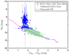 |
Fig. 1 Gaia CMD based on DR2 data for the LG11 sample with Gaia distance and photometry. The pink line represents the main sequence by E. Mamajek (see footnote 1). A residual contamination by giant stars is present. Stars with MG > 5 mag and MKs > 4.6 (the magnitude above which the polynomial relations between photometry and stellar parameters of (Mann et al. 2015) are valid) are highlighted in green. |
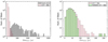 |
Fig. 2 Distance distributions (dBJ18) for various subsamples of the LG11 catalog according to our match with Gaia DR2. Left: giant stars (in gray) and main-sequence stars (in red). Right: zoom into the main-sequence sample (red) and subsample of validated main-sequence stars (green). See text in Sect. 3. |
3.1 M dwarfs in the eFEDS fields
An official X-ray source catalog for the eFEDS fields was produced in parallel with our work and is presented by (Brunner et al. 2022). Our own eROSITA data analysis, which is limited to M dwarfs from the LG11 catalog, is described in Sect. 4.1.1. This analysis involved source detection in the whole eFEDS field. We found 24376 X-ray sources. As a cross-check of our results, we compared our X-ray source catalog with the official catalog (eFEDS_c001_V7_main) produced by (Brunner et al. 2022). First, we found a discrepancy between the X-ray coordinates of our catalog and those in eFEDS_c001_V4_main. We suspect that this is due to an astrometric correction that was used in eFEDS_c001_V4_main to correct for the mean linear offset between the X-ray sources and the Gaia positions of objects in the Gaia-unWISE catalog of candidate active galactic nuclei (AGN) by (Shu et al. 2019). This offset is different for each of the four eFEDS fields and is given in Table 1 of (Brunner et al. 2022). We applied these corrections to the X-ray coordinates of our catalog and verified that this removed the offset between the X-ray positions in our catalog and eFEDS_c001_V4_main. Finally, we calculated the final absolute coordinates (RA_CORR, DEC_CORR) by applying Eq. (1) from (Brunner et al. 2022) to our X-ray catalog.
We then used our catalog with the corrected X-ray coordinates to search for X-ray detections in the LG11-Gaia sample. Thirty-one M dwarfs from our sample lie within the eFEDS field boundaries. We based our match between optical and X-ray position on Gaia coordinates and proper motions from our LG11-Gaia catalog. We first corrected the coordinates of our stars by their P.M. to the eFEDS mean epoch (November 5, 2019), and then we matched them with our final X-ray coordinates (RA_CORR, DEC_CORR). In this way, we found 15 matches within 15”. We cross-checked our detections by matching the P.M.-correctedLG11-Gaia sample with the official eFEDS catalog as well. We found all the 15 stars that we detected in our catalog. The positional uncertainties of all X-ray sources in the eFEDS field were investigated by (Brunner et al. 2022). We verified that for our matches with the LG11-Gaia M dwarfs, the corresponding parameter (RADEC_ERR) is smaller than our match radius.
While it is quite plausible that the M dwarfs from the LG11 catalog emit in X-rays, the limited sensitivity of eROSITA combined with its modest spatial resolution requires a cross-check for other possible optical CTPs to the eROSITA sources. This means that we have to verify the associations between our target stars and the detected X-ray sources. We pursue here a conservative approach, that is, we aim at keeping only those M dwarfs in our sample that we consider secure CTPs to the X-ray sources. We base this assessment on the separation between the optical and X-ray position with respect to that of other Gaia objects in the vicinity.
To determine alternative possible Gaia CTPs for each of the 15 X-ray sources, we performed a reverse match (RM), in which we searched for all Gaia sources within 15” of the X-ray coordinates from our catalog (RA_CORR, DEC_CORR). In this way, we found a total of 21 potential Gaia CTPs, including 14 stars from the LG11-Gaia sample. Then we inspected the separations between the X-ray positions and the Gaia coordinates for the 21 Gaia sources (Sepx,opt). Hereby, we considered the P.M. correction to the mean eFEDS observing date for the Gaia sources that are identified with a star in our input catalog. As a result, the star from LG11-Gaia is the closest Gaia object to an X-ray source for all 14 cases, and these M dwarfs define our list of bona fide eFEDS X-ray emitters. The missing object is a high proper motion star that is not recovered in the reverse match because the P.M. correction can be applied only a posteriori, and a search radius of 15” is too small for this star. Therefore we increased the search radius up to 20”, finding the Gaia source associated with this M dwarf, which is not the closest Gaia counterpart, however. Adhering to our conservative approach, we excluded this star from our LG11-Gaia/eFEDS sample. This sample therefore consists of 14 M dwarfs. All but one of them are also part of our validated LG11-Gaia/eFEDS sample (see Table 1). Finally, we compared the X-ray optical separation (SepX,opt) with the uncertainties on the X-ray positions from our X-ray source catalog (RADEC_ERR). We found that all 14 LG11-Gaia stars in our eFEDS X-ray emitter sample have SepX,opt < 3 x RADEC_ERR, which confirms that the association of the M dwarfs with the eFEDS X-ray sources is consistent with the positional accuracy of eROSITA. These there include one CPM pair that has the same X-ray source associated with each component of the system, but that is resolved by Gaia and 2MASS. We chose to ascribe the X-ray emission to the component that is closest to the X-ray source, and we treated it in the same manner as the single stars. Because the two stars in the CPM pair have similar stellar parameters (M⋆ and SpT), this approach does not influence our results.
In the upper row of Fig. 3 we show the distribution of the distances and spectral types for our LG11-Gaia/eFEDS sample. Fig. 3 (top panels) also highlights the one CPM pair of the sample, as well as the subsample of stars with TESS rotation period, that is, 3 out of 14 stars (see Sect. 4.2). The Gaia source IDs, stellar parameters, and distances for the 14 LG11/Gaia stars in our eFEDS sample are listed in Table 2.
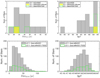 |
Fig. 3 Distribution of Gaia distances from (Bailer-Jones et al. 2018) and spectral types calculated from Gbp – Grp. Top panel: gray histogram is the distribution for the stars from LG11-Gaia in the eFEDS fields. The green contours represent the distance and SpT distribution for those stars observed by TESS. We show the CPM pairs in yellow. Bottom panel: stars from the LG11-Gaia sample identified in the preliminary eRASS1 catalog. For simplicity, we do not show the four CPM pairs here because they represent only 4% of the sample. |
3.2 M dwarfs detected in eRASS1
For the cross-match of our LG11-Gaia catalog with the eRASS1 catalog (v201008), we used the Gaia coordinates, corrected for their proper motions to the rough mean observing date of eRASS1 (March 10, 2020). We cross-matched these extrapolated positions of the M dwarfs with the boresight-corrected coordinates (Col. RA_CORR, DEC_CORR) of the eRASS1 catalog within a radius of 25”. At about 10”, the cumulative histogram of identifications flattens out. The cross-matching radius is a compromise between defining a complete sample and avoiding selecting wrong counterparts. Based on the shape of the cumulative separation distribution, we therefore only considered the matches within 15”. After removing ten stars that are located in the half of the sky that is propriety of the Russian eROSITA consortium the catalog results in 842 X-ray sources. The choice of 15” as identification radius amounts to only ~2% fewer sources than the 25” match radius and ~5% more sources than would be in a 10” radius.
Analogous to the procedure in Sect. 3.1, we performed a reverse match to uncover the Gaia sources that are alternative potential CTPs to the X-ray sources. In this match, we searched for all Gaia sources within 15” of the boresight corrected positions of the 842 eRASS1 sources. This resulted in a total of 2148 potential Gaia counterparts. These multiple optical CTPs should include all 842 LG11-Gaia M dwarfs that were identified in the first match with an X-ray source. In practice, we recovered only 840 of them. This is explained by the fact that two stars are not recovered within 15” because of their high proper motions. These cases are similar to the case discussed in Sect. 3.1, for which a search radius of 15” was too small.
In Fig. 4 we show the distribution of the separations between the Gaia-DR2 and eRASS1 positions in gray. We inspected the separations between X-ray position and Gaia coordinates for all potential Gaia CTPs considering the P.M. correction to the mean eRASS1 observing date for the Gaia sources that are identified with a target star. In this way, we found that the star from the LG11-Gaia list is the closest Gaia object to an X-ray source in 732 cases. Specifically, to find the two stars from the LG11-Gaia sample with very high proper motion that are not recovered in the reverse match, we increased the search radius to 45”. This leads to 734 closest Gaia CTPs that are identified with a star from our LG11-Gaia catalog, that is 87% of the original eRASS1 sample. These objects are shown in blue in Fig. 4. The closest Gaia counterparts to the remaining 108 eRASS1 sources are represented in the red histogram.
Fifteen of the 734 objects for which the closest Gaia counterpart is identified with an LG11-Gaia star have a visual companion. The components of these binary systems are associated with the same X-ray source, thus special attention is needed. By definition of how we identified multiples in the LG11 catalog, these systems are resolved by Gaia. However, 11 of them are associated with a single 2MASS source. Because we cannot determine reliable stellar parameters for these systems, we disregarded them. For the remaining four CPM pairs that are resolved with Gaia and 2MASS but not with eROSITA, we adopted the same approach as for the only binary in the LG11-Gaia/eFEDS sample (see Sect. 3.1), that is, we ascribed the X-ray emission to the component of the binary that is closest to the X-ray position. In one of these four CPM pairs that are resolved with 2MASS, one component has no complete Gaia data, and thus it was removed in the first place from our LG11-Gaia sample (see Sect. 3). Moreover, this component is not the closest component to the X-ray source and would have been removed in any case.
Finally, we removed all stars from the 723 objects for which SepX,opt was higher than three times the uncertainty on the X-ray position in the eRASS1 catalog (RADEC_ERR). This left 673 eRASS1 X-ray sources, and these define our eRASS1 M dwarf sample, LG11-Gaia/eRASS1. Of these, 580 stars are also included in our validated LG11-Gaia/eRASS1 sample (see Table 1).
The Gaia DR2 source IDs, stellar parameters, and distances for the LG11-Gaia/eRASS1 sample are presented in Table 2, and their histograms of distance and SpT are shown in the bottom panels of Fig. 3. The subsample with TESS rotation periods that is described in Sect. 5.2 is overlaid, together with the four stars that have a comoving companion. These distributions are similar to those of the M dwarfs in the eFEDS (displayed in the top panels of the same figure), but their number statistics are higher by more than 20 times. Figure 3 also shows that the subsample observed by TESS is a representation of the X-ray detected stars that is unbiased in terms of distance and SpT.
The source identification is always a compromise between completeness and avoiding to include wrong counterparts. As explained in Sect. 3.1, we aimed to define secure X-ray associations with main-sequence stars from the LG11 catalog at the expense of possibly missing some of them as X-ray emitters. Therefore, we removed all but those M dwarfs that were determined through the above analysis to have the smallest separation to the X-ray source. The nature of the remaining closest Gaia CTPs, that is, those that are not part of the LG11-Gaia catalog, is not of interest to our work. However, a quick assessment can be done with help of a diagram that combines the X-ray-to-optical flux ratio, fx/fG, with Gaia color. On the basis of eROSITA observations from the eFEDS fields, (Stelzer et al. 2022) showed the separation of stars and extragalactic objects in this diagram. In Fig. 5 the closest Gaia CTPs of our reverse match are split into two strongly populated areas. In this figure we only considered the objects with SepX,opt < 3 x RADEC_ERR. The 673 M dwarfs from LG11-Gaia/eRASS1 are located in the lower right corner, including the four stars that have a comoving companion (highlighted in yellow). Most of the remaining closest Gaia CTPs that are not objects from our input catalog are located in the upper left corner of the diagram, which defines the extragalactic region.
Stellar parameters and distances of the eROSITA samples of M dwarfs.
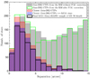 |
Fig. 4 Separation between the X-ray to optical positions for the 842 direct matches of LG11-Gaia stars with the eRASS1 catalog. All 2148 possible Gaia-DR2 CTPs found with the reverse match within 15” are shown in gray. The same objects after the application of their P.M. correction are plotted in green. The red histogram represents the Gaia-DR2 CTP that is closest to each eRASS1 source of our sample, the 734 closest CTPs that correspond to the LG11-Gaia stars studied in this work are shown in blue, and the final LG11-Gaia/eRASS1 sample of 673 M dwarfs is shown in black. |
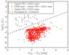 |
Fig. 5 X-ray-to-optical flux ratio vs. Gaia color for the closest optical counterparts to the X-ray sources selected from the match of LG11-Gaia with the eRASS1 catalog. Two distinct regions are visible: the extra-galactic area with high log(fx/fG) values and relatively blue Gaia color, and the star region with lower values of log(fx/fG) and redder Gaia color, separated by the dashed black line we derived from Fig. B3 in Stelzer et al. 2022). The filled red squares are the 673 eRASS1 sources that we identified as M dwarfs (see text in Sect. 3.2), and the filled yellow squares represent the four stars that have a comoving companion. We show only the sources with SepX,opt < 3 x RADEC_ERR. |
3.3 Comparison with the source identification with NWAY
As a cross-check on our source identification procedure, we compared our lists of eROSITA-detected M dwarfs from eFEDS and eRASS1 with the eROSITA sources identified with the NWAY algorithm (Salvato et al. 2018). NWAY is an open-source2 code based on a Bayesian statistics that assigns the probability of being the correct counterpart to every source within a certain distance from the X-ray position. The probability is computed taking into account spatial information (separation between the sources, positional accuracy, and number densities) and priors constructed using a training sample of X-ray sources with a secure counterpart, regardless of their galactic or extragalactic nature. Specifically, for eFEDS (Salvato et al. 2022), the prior was built using optical and mid-infrared photometry from Gaia-DR2 and the Legacy Survey DR8 (LS8; Dey et al. 2019) using 20 705 sources listed in the XXMM-Newton serendipitous source catalogue (3XMM; Rosen 2016). The trained prior was tested on a sample of about 3500 Chandra sources that were assigned artificial eROSITA positional errors. An NWAY match on this simulated dataset indicated a purity and completeness in correct association of about 96%, and only 2% have a possible alternative counterpart.
The comparison of our results with those of NWAY_LS8 showed that all 14 eFEDS X-ray sources that we identified with an LG11-Gaia star are associated with the same star by NWAY. For eRASS1, the NWAY catalog is incomplete because it is limited to the sky coverage of the LS8 survey. For this reason, we can compare the LG11-Gaia catalog and the result from NWAY for only 382 out of 842 (~45%) eRASS1 sources. The comparison is explained in detail in Appendix B. Here we present a short summary for eRASS1, for which the matching was more complicated.
We found an agreement for 93% of our sample. For the vast majority of them (326), the eRASS1 source is identified with our method and with NWAY to an LG11-Gaia M star. In 11 cases, however, we removed an LG11-Gaia star from our final M dwarf list because it is not the closest counterpart to the X-ray source. Here we are more conservative than NWAY because we are restricted to the closest matches, and we therefore lose 3% of the presumed M dwarf X-ray emitters from our final LG11-Gaia/eRASS1 catalog. On the other hand, NWAY-LS8 misses 11 LG11-Gaia stars that we confirmed by visual inspection of sky images as plausible counterparts to the corresponding eRASS1 source.
Although the NWAY-LS8 eRASS1 catalog is not yet complete, we conclude that there is excellent agreement with the results we found from our position-based approach. However, in this preliminary version of the NWAY_LS8 catalog for eRASS1, the coordinates are not corrected for possible proper motion of the sources, resulting in a misidentification of the counterpart for fast-moving objects, and for this reason, we consider our association more reliable in the few dubious cases.
4 Data analysis for the eFEDS fields
4.1 eROSITA
M dwarf stars are soft X-ray emitters. In early versions of our data reduction, we realized that no photons were collected at energies above 5.0keV for the stars detected in our sample. The lowest energy recommended to be used with eROSITA data is 0.2 keV (Predehl et al. 2021). Therefore, we performed the analysis in the 0.2–5.0 keV energy band. In the following, we explain the details of the data extraction and analysis regarding the M dwarfs in the eFEDS fields.
4.1.1 Data extraction
We analyzed the eFEDS c946 processing data using the eSAS-Susers_200602 software release. We extracted eFEDS data in parallel with the construction of the official catalog, therefore both the processing and the software release we used are not the same as were published by the consortium. The data processing provides seven events files in the whole eROSITA energy band (0.2–10.0 keV), one for each telescope and camera system on board eROSITA. We merged the seven files to create one single event and image file filtered for corrupted events in the energy range 0.2–5.0 keV. We calculated the exposure map and the detection mask, which are needed for the source detection, in the same energy band. We computed the background map with the erbackmap routine, using a smooth fit with a smoothing value of 15. Source detection was performed using the ermldet pipeline, for which we adopted a minimum threshold for the detection maximum likelihood of 6.0.
We detected a total of 24 376 X-ray sources in the combined four eFEDS fields. The slight difference with respect to the number of sources in the eFEDS_c001_V4_main catalog (27 910 sources) is most likely to be attributed to the different parameters that were set in the extraction process. These differences have no effect on our study, as we showed in Sect. 3.1, where we anticipated our result for the identification of our M dwarf target list with the eFEDS X-ray sources.
The basic X-ray parameters of the 14 M dwarfs detected in eFEDS are given in Table 3. In particular, we provide the name of the star in LG11 (Col. 1), the X-ray coordinates with their uncertainty (Cols. 2–4), the offset between the proper-motion-corrected optical position and the X-ray coordinates (Col. 5), the 0.2–5.0keV count rate obtained from the source detection procedure (Col. 6), and the detection maximum likelihood in the same energy band (Col. 7).
We also carried out a spectral and temporal analysis for these stars. To this end, we used the srctool routine and selected a circular region for the source (with radius of 30 ”–40 ” depending on the source brightness). The analysis of the light curves and spectra is explained in Sects. 4.1.2 and 4.1.3.
Basic X-ray parameters of the LG11-Gaia/eFEDS and LG11-Gaia/eRASS1 samples.
4.1.2 Spectral analysis
Spectral analysis was performed with XSPEC3 version 12.10. We carried out the spectral fitting only for the 10 out of the 14 detected sources that have more than 30 net source counts. We used a two-temperature thermal model (APEC4) except for one star, which is the faintest of the stars for which we have a reasonable spectrum and which can be described by a one-temperature APEC model.
Each APEC component has three parameters: the plasma temperature (kT), the global abundance (Z), and the emission measure (EM). The emission measure is the square of the number density of free electrons integrated over the volume of the emitting plasma, and it is obtained from the normalization factor of the XSPEC fit combined with the source distance. We fixed Z at 0.3 Z⊙, the typical coronal abundance for late-type stars (Favata et al. 2000; van den Besselaar et al. 2003; Robrade & Schmitt 2005; Maggio et al. 2007), and we left kT and EM free to vary. We computed the mean coronal temperature (Tmean) by weighting the temperatures of the individual APEC components by their EM,
 (1)
(1)
where n = 1, 2 for the two components of the best-fitting model. The parameters of the best-fitting model including the values of Tmean are listed in Table 4, and the spectra are shown in Fig. C.1. One of the ten stars is the binary discussed in Sect. 3.1 that is unresolved with eROSITA, that is, the spectra of two stars are summed. Because the masses of the two components are equal (see Table 2), we can assume the X-ray spectra to be similar, and therefore we treated this spectrum in the same way as the others.
We computed the fluxes in the 0.2–5.0 keV band, fx, with the flux routine provided by XSPEC. For all stars that are too faint for spectral analysis, we calculated a conversion factor (CFeFEDs) for transforming the count rate to flux. We defined CFeFEDs as the ratio of the flux and count rate of each source for which we analyzed the spectrum. In particular, we used the fluxes computed with XSPEC and the count rates we found in the source detection. Then we calculated the mean value,
 (2)
(2)
We excluded the two stars with d.o.f. ≤ 5 (see Table 4) from the calculation of the mean because the coronal temperatures we derive for them are not typical of M dwarf stars, and this is likely the result of the poor statistics of the spectrum. From the eight stars with good-quality spectra, we obtained 〈CFeFEDs〉 = 7.81 × 10⁻¹³ ± 7.48 × 10⁻¹⁴ erg cnt–1 cm–2.
We determined the X-ray fluxes of the four detected stars without a spectral fit (i.e., those with fewer than 30 net counts) and the two stars with a poor spectral fit by combining their count rates with 〈CFeFEDS〉. The X-ray luminosities were determined by combining the fluxes with the distances from Table 2, and the X-ray to bolometric ratios, log(Lx/Lbol) in Table 5 were obtained using the Lbol values derived with the relations of (Mann et al. 2015, 2016). The eFEDS X-ray luminosities are presented in Table 5 together with the ROSAT and TESS parameters derived in the following sections.
We verified with the eFEDS X-ray spectra that the Lx values we calculated for the 0.2–5.0 keV band differ from those for a softer energy band (0.2–2.4 keV) at a level of 1% or lower. This can be easily understood from Fig. C.1, where the spectra drop steeply above ~1 keV. Therefore, we use the broader standard eROSITA band in the remainder of this paper for our eROSITA detections, also when we compare eROSITA and ROSAT measurements.
X-ray spectral parameters for the ten M stars in eFEDS with more than 30 counts in the 0.2–5.0 keV band.
Measurements of X-ray activity and rotation derived by us from eROSITA, ROSAT, and TESS data.
4.1.3 Light-curve analysis
Each of the four eFEDS fields was scanned by eROSITA in the direction of the longer side of the individual fields. Thus, eROSITA has visited a given object within the eFEDS fields several times with a time lapse between one and the next visit that depends on the position of the object. As a consequence of this observing mode, light curves of individual sources are defined by short (<100 s) intervals of data taking (called one ‘visit’), separated by longer data gaps during which the satellite scans through the rest of the field, turns around, and approaches the source again. Generally, the length of the data gaps alternates between two values, except for sources that are located in the middle of the eFEDS fields along the scanning direction, where all data gaps have an approximately equal length.
We performed the light curve extraction with the dedicated source products pipeline, srctool, which is part of the eSASS software. We worked in the energy band between 0.2 and 5.0 keV, and we used the same source and background regions as we adopted for the spectral analysis.
As explained above, in survey mode, a regularly binned light curve is dominated by data gaps. We therefore used the REGULAR option to produce light curves with regularly spaced bins in which time intervals without data are automatically discarded. We performed tests with different bin sizes to identify the best value for each source in order to avoid bins with a very low number of counts and a correspondingly large uncertainty because they start near the end of a visit. As explained above, because the visits are not regularly spaced, a large bin size was required to reach this goal. The binning we determined from our tests is between 1 and 3 ks; this was chosen individually for each source. For stars located in the scanning direction near the edge of the eFEDS fields, this means that we averaged over two successive visits.
The light curves of all 14 stars from our sample that are detected in the eFEDS fields are shown in Fig. D.1, where the individual bin size is indicated for each star in the legend. The uncertainties of the count rate are automatically calculated by the eSASS pipeline, and they depend on the uncertainties of the source and background counts, the fractional telescope collecting area, and the fraction of the time bin that overlaps with the input good time intervals (GTIs) that have been calculated by the eSASS pipeline during the extraction of the events file. During its first and last visit, the source is located at the edge of the field of view and the fractional telescope collecting area and the fractional temporal coverage become smaller. Consequently, the error bars increase.
A systematic analysis of the variability of all sources detected in the eFEDS field is presented by (Boller et al. 2022). This variability study refers to all objects in the official eFEDS source catalog, which comprises our 14 detected M dwarfs. We extracted the variability metrics for these 14 stars from the catalog of (Boller et al. 2022). Specifically, this catalog provides the normalized excess variance (NEV) as defined by (Boller et al. 2016) and its uncertainty. The eFEDS variability tests carried out by (Boller et al. 2022) on the full eFEDS sample were performed on light curves with bin sizes of 100 s. The ratio of these two quantities represents the probability that the source is variable in units of Gaussian σ. We find that five of the LG11-Gaia/eFEDS sample have a well-determined NEV and its uncertainty. In the eFEDS fields, the net count statistics is low for most sources, such that the NEV is unconstrained. Only for one of the M dwarfs that is identified as variable is the NEV σ > 3, and another one has σ > 2.5. These two stars are PM I09161+0153, the brightest star in our sample (in terms of X-ray count rate), for which the visual inspection of the light curve indicates a likely ongoing flare at the beginning of the observation, and PM I09201+0347, which shows a smoother and longer-lasting variability throughout the eFEDS light curve.
4.2 TESS
To retrieve TESS data, we uploaded our target list of the 14 M dwarfs from the LG11-Gaia/eFEDS catalog to the Barbara A. Mikulski Archive for Space Telescopes (MAST) interface and found TESS data for 13 stars. We used the J2000 coordinates from LG11 for the match, with a match radius of 1”. Because the pixel scale of TESS is so large (21” per pixel), a P.M. correction or its omission does not influence the result. Many stars have two TIC numbers, and we determined the correct TIC counterpart by comparing the magnitudes of the multiband photometry provided in the TIC with the values listed for the LG11 star in Simbad and ESASky.
All but one of the 13 stars have short (two-minute) cadence light curves. The remaining star was observed in full-frame image (FFI) mode only. The observation of the eFEDS fields was performed by TESS in its Sectors 7 and 8 during January and February 2019, and we downloaded the data from the MAST portal.
4.2.1 Analysis of the two-minute cadence light curves
For our analysis, which consisted of three steps, we used the pre-search data conditioning simple aperture photometry (PDCSAP) light curves. TESS assigns a quality flag to all measurements, including data that are of poor quality, but also data that might be of lower quality or could cause problems for transit detection after applying a detrending software (Thompson et al. 2016). Hence, removing all flagged data points by default could impede the detection of real astrophysical signals or the interpretation of systematics. Therefore, we removed all flagged data points except those of ‘impulsive outliers’ (which could be real stellar flares) and ‘cosmic ray in collateral data’ (bits 10 and 11) in step 1 of the analysis. In a second step, we normalized the light curves by dividing all data points by the median flux.
The third analysis step is the search for rotation periods. To this end we used three different methods, the generalized Lomb-Scargle periodogram (GLS; Zechmeister & Kürster 2009), the autocorrelation function (ACF), and fitting the light curves with a sine function. We first used this approach on data from the K2 mission, and all details on our period search can be found in (Stelzer et al. 2016) and (Raetz et al. 2020). For the analysis with GLS we had to bin the data by a factor of 3 because the implementation we use5 can only deal with up to 10000 data points.
4.2.2 Analysis of the full-frame images
Because one of our targets with available TESS data does not have a light curve with a 2-min cadence, we decided to extract the long (29-min) cadence light curves of all 13 targets from the FFIs. To create a light curve, we performed aperture photometry. Instead of using all FFIs, we made use of the so-called postcards, which are an intermediate data product from the FFI analysis tool ELEANOR (Feinstein et al. 2019). Postcards are 148 x 104 pixel background-subtracted cutout regions of the FFIs that are time-stacked, including all cadences for which observations are available. We converted the postcard cubes into individual fits images. Sectors 7 and 8 include 1093 and 968 cadences, respectively. Photometry was performed following the procedures described by us in (Raetz et al. 2016), for instance. In short, for the aperture photometry with ten different aperture radii, we used a user script based on the standard IRAF routine phot. Our script allows us to obtain simultaneous photometry of all stars in an image. For this purpose, a list of the pixel coordinates of all detectable stars was created using SOURCE EXTRACTOR (SEXTRAC-TOR; Bertin & Arnouts 1996). As the positions of the stars on the CCDs do not change during a sector, a single file with pixel coordinates was used for all cadences. Finally, we derived differential magnitudes using an optimized artificial comparison star (Broeg et al. 2005). Because TESS has an image scale of ~21 arcsec per pixel, we found the optimal aperture radius for all targets to be 2 pixels. The resulting light curves of sector 8 show strong systematic effects at the beginning of the observations and after the observation gap caused by the data downlink at Earth perigee. We removed all affected data points, leading to final light curves with 1093 and ~650 data points for sectors 7 and 8, respectively.
The long-cadence light curves show smaller scatter than the short cadence light curves. Figure 6 shows as an example the comparison of the 2-min cadence PDCSAP light curve and the 30-min light curve extracted from the FFIs for PMI09034-0023 (TIC 893123) observed by TESS in Sector 8. Although the two light curves agree within their error bars, the scatter is much lower in the FFI light curve. For this particular star, the FFI light curve indicates a double-hump shape, in contrast to the single sinusoidal shape in the PDCSAP light curve. Furthermore, the detrending of the strong systematic effects of Sector 8 might introduce artifacts that could cause an incorrect determination of the rotation period. Therefore we applied the period search as explained in the previous section to the long-cadence light curves as well.
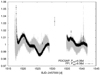 |
Fig. 6 Comparison of the pipeline-produced PDCSAP light curve of PMI09034-0023 (TIC 893123, gray) and our own photometry (black) extracted from the full frame images. Within the error bars, the two light curves agree with each other, while the scatter is much larger for the light curve with the two-minute cadence. The shape of the light curve is different, however, which results in different estimates of the rotation period. |
4.2.3 Note on the binary star
Our list of the 13 LG11-Gaia/eFEDS stars observed with TESS includes the one close visual binary pair from Sect. 3.1. With the large pixel scale of TESS, these stars cannot be resolved individually. Consequently, the automatic pixel masks of the short-cadence data that are centered on the stellar position are slightly offset from each other, resulting in slightly different light curves. For the FFI, we defined the pixel mask ourselves, and we only created one light curve per binary pair.
4.2.4 Outputs of the light-curve analysis
For each target, we obtained six values for the rotation period: three for the long-cadence light curves, and three for the short-cadence light curves. By-eye inspection of the phase-folded light curves determined the best-fitting period. If several methods resulted in a similar value, we computed the average. The standard deviation was used to determine the uncertainties. In addition, we used the formulas given in (Gilliland & Fisher 1985) to calculate an error for the rotation period. As the final uncertainty, we adopted the maximum of the standard deviation and the calculated error. We detected rotation periods for five targets from the LG11-Gaia/eFEDS sample. By repeating the period search on the residuals of the light curve after subtracting the dominant period, we found that one star shows an additional shorter period. Another star exhibits a double-hump shaped light curve; we discussed this in Sect. 4.2.2. We excluded these two stars with ambiguous period signal from our quantitative analysis, although we show them in the figures with separate symbols from the reliable sample. To summarize, only 3 of the 13 eFEDS M dwarfs have a reliable period detection, and they represent our LG11-Gaia/eFEDS/TESS sample (see Table 1). All of them are validated with the (Mann et al. 2015) relations. The most significant period is listed for all five stars in Table 5, and a flag is provided for those that are not considered for the reasons described above.
5 Data analysis for eRASS1
5.1 eROSITA
In principle, the same analysis steps described and carried out for the eFEDS data in Sect. 4.1 can be applied to eRASS data. However, we defer this in-depth study to a future work.
The X-ray parameters used in this work were directly extracted from the eRASS1 catalog. We list in Table 3 the same parameters as for the X-ray detections found in the eFEDS fields for the 673 LG11-Gaia/eRASS1 stars. Next to the LG11 name (Col. 1), we provide the X-ray coordinates with their uncertainty (Cols. 2–4), the offset between proper-motion-corrected optical position and the X-ray coordinates (Col. 4), the 0.2–5.0 keV count rate (Col. 5), and the 0.2–5.0 keV detection maximum likelihood (Col. 6).
Because a systematic analysis of spectra and light curves such as that of Sects. 4.1.2 and 4.1.3 is beyond the scope of this work, we used the conversion factor 〈CFeFEDS〉 derived from the eFEDS data to compute the X-ray fluxes for the eRASS1 detected M dwarfs. X-ray luminosities and Lx/Lbol ratios were then determined with the distances and Lbol values from Table 2. The Lx and Lx/Lbol values are listed in Table 5, together with the same parameters for the eFEDS detections.
5.2 TESS
Analogous to the case of eFEDS (Sect. 4.2), we loaded the list of 673 X-ray detected stars from our LG11-Gaia/eRASS1 catalog into MAST to define the sample of stars with TESS data, and we matched it with the target list of TESS using the J2000 coordinates in LG11 with a match radius of 1”. We found that 476 of the LG 11-Gaia M dwarfs detected in eRASS1 have been observed with TESS. We recall the all-sky nature of eRASS1, which implies that the M dwarfs from this sample are distributed over all TESS sectors. Of the 476 stars, 125 were observed in multiple sectors. The subset of the LG11-Gaia/eRASS1 sample observed with TESS includes three of four comoving binary systems from Sect. 3.2.
For the stars from the LG11-Gaia/eRASS1 sample, we examined only the two-minute-cadence TESS data in the way described in Sect. 4.2.1. The adopted values for the rotation periods were determined with the procedure described in Sect. 4.2.4.
We were able to determine rotation periods for 217 stars, but we consider 39 of these periods to be not reliable because the period is longer than half the duration of the observation. The periods of these stars are flagged in Table 5. Through inspection by eye, we found that three more stars show a second period that was not identified as the dominant period with our period-search methods, and an additional three stars have a light curve that looks double-humped like the light curve in the eFEDS sample discussed in Sect. 4.2.2. We removed these six stars from the sample, and we defined this sample as LG11-Gaia/eRASS1/TESS for our further analysis. This sample comprises 172 stars. We note that for completeness, the removed six stars with ambiguous Prot are shown in the figures distinguished with the plotting symbol from the stars from the LG11-Gaia/eRASS1/TESS sample. The period with the highest significance is given in Table 5, together with a flag that identifies the stars that were removed from the rotation sample as described above. Taking the calibration range of (Mann et al. 2015) into account, we obtained a validated LG11-Gaia/eRASS1/TESS of 135 stars.
6 Results and discussion
6.1 eROSITA M dwarf population
We studied the X-ray emission of the M dwarfs from the LG11 catalog with matches in Gala DR2 in two different eROSITA surveys: the eFEDS observation, which covers 142 sq. deg in the southern hemisphere, and the first full all-sky survey, eRASS1. These two eROSITA samples together provide the X-ray luminosities of 687 M dwarfs, which exceeds our previously compiled sample (Magaudda et al. 2020) in size by more than a factor of two, historical samples from RASS by a factor of 7 (NEXXUS; Schmitt & Liefke 2004), and the sample from Einstein by a factor of 24 (Fleming et al. 1988).
Thirty objects in the list of 8229 main-sequence M dwarfs provided by LG11 that have a Gaia DR2 counterpart are located in the eFEDS fields. This matches the all-sky space density average (30 out of 142 ≈ 8229 out of 41253 stars per sq.deg) almost exactly. We detected 14 of these 30 M dwarfs, which is nearly 50% of the sample. The average space density of X-ray detected M dwarfs in the eFEDS sample therefore is 14 out of 142 ≈ 0.10 stars per sq.deg.
Our analysis of the eRASS1 catalog has provided the largest sample of X-ray emitting M dwarfs to ate, namely 673 stars, which is a detection rate of 8.3% of our input sample LG11-Gaia. The eRASS1 space density of X-ray detected M dwarfs is 673 out of 20626 ≈ 0.033 stars per sq.deg (considering half of the sky comprised in our version of the eRASS1 catalog). This is lower by a factor three than for eFEDS, which can be explained by the shorter exposure time (on average) during the all-sky survey.
The typical eFEDS exposure time is ~1 ksec per sky position. The exposure time, and therefore the flux limit, during eRASS strongly depends on the sky position and is therefore not a universal value for a sample distributed over the sky. We can, however, give a rough value of flim,eRAss1 ~ 3 × 10–14erg cm–2 s–1. At this value, the distribution of fluxes detected for our M dwarfs drops steeply, and the flux of only ~2% of the detections is lower than this. Defining the flux limit in the same way as for eRASS1 (i.e., as that value fx that is exceeded by 98% of the stars in the sample), we find flim,eFEDS ~ 2 × 10⁻¹⁴ erg cm−2 s−1, which is slightly deeper than that of eRASS1. We therefore conclude that the eFEDS and eRASS1 detection statistics are qualitatively consistent with each other. A more detailed comparison, however, is prohibited by the low number statistics in the eFEDS fields.
6.2 Mass-dependence of activity and rotation
Both activity and rotation are known to depend on stellar mass. While a detailed investigation of the rotation-mass relation has come within reach with the Kepler mission, statistical samples for X-ray to mass studies within a spectral subclass have not been available so far. In Fig. 7 we show X-ray activity diagnostics and rotation periods versus stellar mass, that is, Lx – M⋆ (left panel), Lx/Lbol – M⋆ (right panel), and Prot – M⋆ (bottom panel) for M dwarfs. For the X-ray to mass relations, we considered the LG11-Gaia/eFEDS and LG11-Gaia/eRASS1 samples, while for the Prot – M⋆ relation, we show the X-ray detected M dwarfs with rotation period, that is, the LG11-Gala/eFEDS/TESS and LG11-Gaia/eRASS1/TESS samples and the stars with two periods (green symbols) that are not considered in our quantitative analysis. We include in all panels data from (Magaudda et al. 2020) (in gray), which comprise new XMM-Newton, Chandra, and K2 mission observations and a collection of results from the literature that we updated in (Magaudda et al. 2020).
The X-ray luminosities from (Magaudda et al. 2020) were extracted in the ROSAT energy band (0.1-2.4 keV). As explained in Sect. 4.1.2, our use of a different energy band for the eROSITA data (0.2–5.0 keV) does not bias the results. (Magaudda et al. 2020) extracted distances from Gaia-DR2 parallaxes (Gaia Collaboration 2016, 2018a) and validated them using (Lindegren et al. 2018) and our own quality criteria. To be consistent with the LG11-Gaia/eROSITA samples, we retrieved Gaia distances from BJ18, and for Fig. 7 and the subsequent analysis in Sect. 6.3, we cleaned the sample from (Magaudda et al. 2020) by removing all stars that lack Gaia photometry and/or distance and the nine upper limits presented in the original sample. To calculate the stellar parameters, we followed the recipes described in Sect. 3. Moreover, we identified and removed 13 stars with MG < 5 mag. These updates are motivated by a comparison of masses and spectral types analogous to the one carried out for the LG11 catalog in Sect. 3. With these restrictions, the sample from (Magaudda et al. 2020, henceforth referred to as Gaia-Magaudda 2020) includes 259 stars with 0.15 ≤ M⋆/M⊙ ≤ 0.85.
In Fig. 7 we consider the full mass range obtained from the MKs values of the stars, but strictly speaking, masses above 0.7 M⊙ are not validated because the MKs values of these stars are beyond the calibrated range of the relation from (Mann et al. 2015). We decided to show the full mass range because there is no obvious qualitative change in the Lx – M⋆ relation at this boundary, and we take this as a justification to extrapolate the underlying M⋆ – MKs relation.
Figure 7 shows that for a given stellar mass, we observe a spread of 2–3 orders of magnitude in the X-ray activity level, except for the lowest (M⋆ ≲ 0.3 M⊙) and highest masses (M⋆ ≳ 0.7 M⊙), where the spread is smaller. At the low-mass end, only the upper part of the Lx values is clearly detectable in our flux-limited eROSITA observations, while the high-mass end corresponds to the transition to spectral type K, which is not fully sampled in the LG11 catalog. We calculated the median and standard deviation in mass bins of ∆M⋆ = 0.1 M⊙ for the combined M dwarf sample from the literature and from this eROSITA study. The resulting values are overlaid on the data in red for the validated mass range. In the intermediate-mass range, which is best sampled by our catalog, the standard deviation is ~0.73 for Lx and ~0.75 for Lx/Lbol, in logarithmic scale. We fit the two X-ray to mass relations for the combined literature and eROSITA sample with a linear function in log-log space, finding a slope of +2.84 ± 0.25 for Lx – M⋆ and –0.10 ± 0.10 for Lx/Lbol – M⋆. The best-fit relations are given in Table 6, and we display the fits in Fig. 7. Interestingly, the historical study of M dwarfs by (Fleming et al. 1988) on a very limited sample (~30 field M stars with 0.15 ≤ M⋆/M⊙ ≤ 0.6) reported a similar slope to ours for the Lx – M⋆ relation within the uncertainty. The numbers for the average X-ray activity level across all masses in the M dwarf regime must be considered an upper limit because even in a volume of 10 pc around the Sun, ~40% of the M dwarfs are still undetected in X-rays (Stelzer et al. 2013). We show the X-ray activity level for M⋆ = 0.5 M⊙ in Cols. 3 and 5 in Table 6. We defer a more detailed discussion and comparison to literature studies to Sect. 6.3.
In the bottom panel of Fig. 7, we inspect the Prot – M⋆ relation of our samples in comparison to data from (McQuillan et al. 2013), which cover the mass range of 0.3–0.55 M⊙ with selection criteria based on Teff and log g values from the Kepler input catalog, and (McQuillan et al. 2014), which is the extension of that study to all stars with Teff < 6500 K. The rotation periods of the sample from (Magaudda et al. 2020) were extracted from light curves of the K2 mission, the MEarth project, and ground-based observations, and they cover a broad range of values from 0.1 d to ~100 d. As explained by (McQuillan et al. 2014) and (Stelzer et al. 2016), the Prot – M⋆ relation shows a bimodal period distribution for lower masses and an upper envelope of the period distribution that increases for decreasing masses. Similar results were found, for instance, by (West et al. 2015) and
(Newton et al. 2017) by studying the chromospheric activity of M dwarfs through their Ha emission. They observed higher Prot for lower-mass stars (M⋆ ≤ 0.25 M⊙), which also appear to be less active than the more rapidly rotating and more massive stars. In particular, (Newton et al. 2017) proposed a mass-dependent rotational period threshold for the ignition of the Hα emission. Furthermore, they argued that the paucity of mid- to late-M dwarfs with intermediate rotation periods in their sample is probably caused by a period range over which stars quickly lose angular momentum. The boundary between active and inactive M stars coincides with the rotation period at which the rapid evolution phase ceases, suggesting that the Ha emission and M dwarfs with intermediate Prot are connected. In the data compiled by (Magaudda et al. 2020) (gray in Fig. 7), we encountered the same paucity of M stars in the intermediate Prot regime at the lowest masses, and we confirm the upward trend for stars with the longest periods and lowest masses.
The periods in our eROSITA and TESS samples are biased because TESS stares at a given field for only about a month, and we considered periods longer than about half the duration of a sector light curve to be unreliable. The eROSITA/TESS sample of LG11-Gaia stars is therefore located in the range of fast rotators, which is a sparsely populated region in unbiased surveys for stellar rotation periods. Interestingly, TESS covers this regime entirely, that is, up to the transition (at Prot ~ 10 d) at which the bulk of the M dwarfs are situated. With eRASS1, we added some very low-mass stars with fast rotation to the Prot - M⋆ relation, showing that the lowest-mass stars span the widest range of periods, and that the vast majority of rotation rates in between the extremes have not yet been covered by X-ray observations for this mass range.
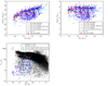 |
Fig. 7 X-ray activity and rotation vs. mass: blue and pink show the eRASS1 and eFEDS M dwarf samples, respectively, and gray shows the revised sample from (Magaudda et al. 2020); see the legend inside the panels for other literature data and highlighted specific subsamples. In the top panels, the median and the standard deviation of the data are presented in red for bins with a width of 0.1 M⊙. Top left: X-ray luminosity vs. mass and best fit (cyan). Top right: X-ray over bolometric luminosity vs. mass and best fit (cyan). Bottom left: rotation period vs mass; for the stars with double-humped TESS light curves, the shorter of the two periods is shown. |
Results obtained from fitting Lx – M⋆ and L/Lbol – M⋆ for the full sample (LG11-Gaia-eFEDS, LG11-Gaia-eRASS1 and Gaia-Magaudda20) and for the saturated subsamples, i.e., stars with Prot ≤ Psat; see Sects. 6.2 and 6.3 for details.
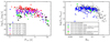 |
Fig. 8 X-ray activity-rotation relations. Left: X-ray luminosity vs rotation period with mass-color code in steps of 0.1 M⊙. Right: X-ray luminosity as a fraction of bolometric luminosity vs. Rossby number. See the legend, the caption of Fig. 7, and the text in Sect. 6.3 for the subsamples we display. |
6.3 Rotation-activity relation
In the previous section, we showed that with the new eROSITA/TESS sample, we can study the regime up to Prot ~ 10 d, which corresponds to the saturated regime in the rotation-activity relation. Here, we present the X-ray activity-rotation relation we constructed with the results obtained from eROSITA and TESS observations of the validated LG11-Gaia sample, combined with the stars of the sample from (Magaudda et al. 2020), revised as described in Sect. 6.2, which we also restricted to the stars with MKs in the calibration range of (Mann et al. 2015). This validated Gaia-Magaudda20 sample contains 197 M dwarfs. The plots of X-ray activity versus rotation diagnostics are shown in Fig. 8.
Sections 4.2.4 and 5.2 showed that 489 out of 687 LG11-Gaia/eFEDS and LG11-Gaia/eRASS1 stars are detected eROSITA X-ray detection and are also observed by TESS observations. The sub-sample with reliable TESS rotation period consist of 3 and 135 stars for eFEDS and eRASSl, respectively. The new eROSITA/TESS data therefore nearly double the sample that was previously available for studies of the X-ray activity-rotation relation.
Previous studies (Pizzolato et al. 2003; Wright et al. 2011, 2018; Wright & Drake 2016; Magaudda et al. 2020) revealed two different regimes of the rotation-activity relation: a saturated regime for fast-rotating stars with Prot ≤ 10 d, and an unsaturated regime for slowly rotating stars with Prot > 10 d. These two regimes are clearly present in Fig. 8, but the new eROSITA/TESS samples cover only the saturated part. In the left panel, we present the activity-rotation relation with a color-mass code in bins of 0.1 M⊙. In the saturated regime, a systematic decrease in average X-ray luminosity with decreasing stellar mass is evident, reflecting the trend that is seen in the direct Lx – M⋆ relation for the full sample, which is displayed in Fig. 7. A further investigation of the X-ray activity level in the saturated regime through fitting the data in X-ray to rotation space and a consideration of the sample biases will be presented by Magaudda et al. (in prep.).
In the right panel of Fig. 8, we use the same color-code as in Fig. 7 to distinguish the various samples used in this work for the rotation-activity relation in terms of the X-ray fractional luminosity (Lx/Lbol) versus Rossby number (RO). The Rossby number is defined as the ratio of the rotation period and the convective turnover time (τconv), which is not a directly observable parameter. Here as well as in (Magaudda et al. 2020), we adopted the empirical calibration of τconv with V – Ks magnitude provided by (Wright et al. 2018). The Rossby numbers obtained from the TESS rotation period values are provided in Table 5. The right panel of Fig. 8 shows that switching from the Lx – Prot space to the Lx/Lbol – RO space, the rotation-activity relation changes its structure. For the eROSITA/TESS samples, the most relevant difference between the two diagrams is the decrease in vertical spread in the saturated regime when the X-ray luminosity is normalized by the bolometric luminosity.
We can use the unprecedented statistics in the saturated regime to examine the mass dependence of the X-ray emission of fast rotators within the M spectral class. Fast rotators represent the younger population of M dwarfs (age < 1 Gyr, according to Magaudda et al.) for partially convective stars, and up to ~4 Gyr for stars with M⋆ < 0.4 M⊙). To this end, we defined a subsample of M dwarfs by combining our new data and the revised validated Gaia-Magaudda20 sample that we limited to stars with detected rotation period that fulfill the criterion Prot < Psat = 8.5 d. Here Psat is the period at the transition from the saturated to the unsaturated regime. Our adopted value for Psat is the one from (Magaudda et al. 2020) in their full M dwarf sample. Figure 8 shows that with this choice, we avoid including unsaturated stars.
The distributions of X-ray activity versus stellar mass for this fast-rotator sample are shown in Fig. 9. As in Fig. 7, we also display the median and standard deviation of the data in bins with a width of 0.1 M⊙. The linear fit obtained for these stars (blue) yields a slope of 3.10 ± 0.27 for Lx and 0.36 ± 0.25 for Lx/Lbol (see Table 6). For comparison, we insert in Fig. 9 the fits obtained in Sect. 6.1 for our full sample and the result of (Preibisch & Feigelson 2005), who performed the same type of linear fit, but for the T Tauri stars in the Orion Nebular cluster (ONC) with M⋆ < 2 M⊙.
First, we can observe that the exclusion of unsaturated stars barely changes the slope of the Lx – M⋆ relation, but it converts the marginally negative slope in Lx/Lbol – M⋆ space into a marginally positive one. The dedicated studies of slowly rotating fully convective stars by (Wright & Drake 2016); (Wright et al. 2018) reported that the unsaturated regime is dominated by the more massive M dwarfs, which have shorter spin-down timescales, however. In the center of our mass distribution (≈0.5 M⊙), the X-ray / mass relation for the saturated subsample is shifted by ~0.5 dex to higher activity levels than in the full sample. Because the full sample is likely still incomplete and includes the saturated subsample, this poses only a lower limit to the change in X-ray emission level between <1 Gyr and several Gyr old M dwarfs.
The slope of Lx – M⋆ we derived for our field M dwarfs is significantly higher than the one for the ONC from (Preibisch et al. 2005) (βONC = 1.44 ± 0.10). The X-ray luminosities of the Orion sample are shifted upward with respect to the field dwarfs because of the young age of the ONC. The decrease in Lx – M⋆ relation between the ONC and our saturated subsample encodes the evolution between 1 Myr and ≲1 Gyr, which is ~2.0 dex in logarithmic space for the low-mass end (~0.15 M⊙) and ~0.8 dex at the high-mass end (0.7 M⊙). In terms of normalized X-ray luminosity, our two M dwarf distributions are within the uncertainty of the Lx/Lbol – M⋆ relation of the ONC. Remarkably, our saturated sample, which spans the same range of periods as the ONC (e.g., Choi & Herbst 1996; Rodriguez-Ledesma et al. 2009), is located in the upper half of the ONC distribution, which means that the Lx/Lbol levels of fast-rotating field M dwarfs are at least as high as thos of pre-main-sequence stars. As noted by (Preibisch et al. 2005), this apparently reduced activity level for the pre-main-sequence stars arises because the ONC sample includes accreting stars, which have lower X-ray luminosities than nonaccretors.
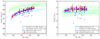 |
Fig. 9 X-ray activity vs mass for the validated samples (see legend in Figs. 7 and 8) restricted to the saturated stars, i.e., stars with Prot ≤ 8.5 d, best fit (violet) and median plus standard deviation of the data (red) in bins of 0.1 M⊙. The fit to the young stars in the Orion Nebular cluster provided by (Preibisch et al. 2005) is also shown, together with the standard deviation of this fit (green) and the best fit we found for the full M dwarf sample presented in the top panels of Fig. 7 (cyan). Left: X-ray luminosity vs. mass. Right: X-ray over bolometric luminosity vs. mass. |
6.4 Relation of coronal temperature to luminosity
In Fig. 10 we show the eFEDS M dwarfs whose X-ray temperature and luminosity were determined from the spectral analysis (see Table 4) in a scatter plot. As we explained in Sect. 4.1, we excluded the two stars with d.o.f. ≤ 5 because the statistics of their spectra is poor. For comparison, we also show the results from (Johnstone & Güdel 2015) for a sample of GKM stars collected by these authors from the literature and the recent XMM-Newton measurement for the planet host star GJ 357 from (Modirrousta-Galian et al. 2020). Star GJ 357 is a representative of the faintest and coolest M dwarf coronae studied so far.
The stars from the (Johnstone & Giidel 2015) sample are among the most well-known dwarf stars in the solar neighborhood, and for some of them, the stellar parameters have been determined very precisely in dedicated studies. However, for the sake of homogeneity, we selected the M dwarfs from their sample with the same procedure, explained in Sect. 3, as we applied to the full LG11 catalog. Specifically, we computed the SpTs from GBP – GRP (see Sect. 3 and footnote 1). This provided six M dwarfs, the same as are given M spectral type in SIMBAD. We note in passing that all of them except SCR J1845-6357 (henceforth SCR1845) lie within the validation range of the (Mann et al. 2015) relations. According to the literature, SCR J1845-6357 is a late-M dwarf (SpT M8.5; Robrade et al. 2010), and its MKs value is slightly higher than the upper boundary of the range calibrated by (Mann et al. 2015). The six stars we selected have M⋆ ≲ 0.7 M⊙ according to the (Mann et al. 2015) relation. These stars are highlighted as filled black circles in Fig. 10. Their X-ray properties are adopted from (Johnstone & Güdel 2015), except for the X-ray luminosity of Prox Cen, for which we used the value from (Ribas et al. 2016), log Lx [erg s−1] = 27.
The six M dwarfs from (Johnstone & Gudel 2015) alone delineate a rather well-defined correlation between Tx and Lx, and GJ 357 is roughly consistent with an extension of this relation at the faint and cool end. We note that (Johnstone & Gudel 2015) have distinguished stars in two mass bins, above and below M⋆ = 0.65 M⊙. They determined the stellar masses from B - V colors using the evolutionary models of (An et al. 2007). In this way, they included four more stars in their low-mass group with respect to the six we selected. In Fig. 10 these stars are found among the open circles, where they are marked with a cross. These stars have SpT early-K, and they are displaced downward with respect to the M dwarfs.
The eROSITA sample comprises a narrow range of X-ray luminosities that is limited by the sensitivity of the eFEDS observation. However, in contrast to the literature sample, the stars from eFEDS display a significant spread in terms of Tx. As explained in Sect. 4.1.2, the X-ray luminosities of the eFEDS stars are insensitive to variations in the energy band within the typical range of ROSAT and eROSITA data. The mean upward shift of the eFEDS sample is therefore unlikely to be the result of an observational bias. Moreover, scatter is seen within the eFEDS sample itself, which has been analyzed in a homogeneous way. We caution, however, that the star with the highest Tx value is the only one from the eFEDS sample that was analyzed with a 1 -T spectral model, and it presents evidence for variability in its light curve (see Appendix D).
A larger database of homogeneous coronal temperature measurements for M dwarfs is needed to explore the Tx – Lx relation, and in particular, its spread and a possible influence of flares. The eRASS represents a such valuable database. While a detailed spectral analysis of hundreds of M dwarfs detected in eRASS will be presented in a later work, here we use hardness ratios (HR) as a proxy for the coronal temperature.
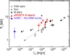 |
Fig. 10 Coronal temperature vs. X-ray luminosity for M dwarfs with eROSITA spectra (red circles), compared to FGKM stars from (Johnstone & Gudel 2015) (black circles) for which according to our updated analysis there are six M dwarfs (filled circles and individually labeled: 1 – AU Mic, 2 – EV Lac, 3 – AD Leo, 4 – YZ CMi, 5 – Prox Cen, and 6 – SCR 1845). Stars labeled low-mass (M⋆ ≤ 0.65 M⊙) in (Johnstone & Gudel 2015) but which have SpT K are marked with a cross. At the faint and cool end lies the planet-hosting M dwarf GJ 357 from (Modirrousta-Galian et al. 2020) (blue circle). |
6.5 eROSITA hardness ratios
The analysis of hardness ratios does not involve the stellar parameters. Based on the argument put forth in Sect. 6.1, we therefore also consider the stars outside the validation range of the (Mann et al. 2015) relations.
We used the three energy bands provided by the eRASS1 catalog, the soft (0.2-0.6 keV), medium (0.6-2.3 keV), and hard (2.3–5.0 keV) band, to define hardness ratios as follows:
 (3)
(3)
 (4)
(4)
where HR1 is the count rate ratio of the medium and soft energy bands, while HR2 is calculated between the hard and the medium energy bands. The two hardness ratios are given for the eROSITA -detected stars in Table 5.
In Fig. 11 we show the scatter plot of HR2 versus HR1 for the LG11-Gaia/eRASS1 and the LG11-Gaia/eFEDS sample. A large fraction of the stars (~60%) have no counts in the hard energy band (HR2 = – 1), and most of them are clustered at 0.2 ≤ HR1 ≤ 0.6 (~65% of the total sample). This range of HR1 includes all but two stars for which we analyzed the eFEDS spectra. We thus can conclude that moderately positive values of HR1 are associated with soft plasma of ≲ 0.5 keV. According to (Foster et al. 2022), this range of HR1 values corresponds to plasma of 0.2…0.35 keV. We caution, however, that their analysis is based on a 1 -T model, while our sample shows that two temperatures are required to adequately describe the eROSITA spectra of M dwarfs. Therefore, the calibration between HR1 and kT from (Foster et al. 2022) may not be applicable to our sample.
Concerning HR2, the curious objects are those that are not at the soft limit, that is, those with HR2 > – 1. They can be broadly distinguished into two groups: one is clustered near the HR2 soft bound and intermediate HR1 values (~30% of the whole sample), and the other scattered throughout the parameter space (~10%). The first are likely represented by M dwarfs with a slightly hotter corona than those at HR2 = – 1, while for the second group, a plausible hypothesis for their harder spectra is flaring activity. The analysis of all individual eRASS1 light curves in a future study will allow us to further examine this interpretation.
6.6 X-ray variability
We analyzed the eROSITA light curves of 14 M dwarfs detected during eFEDS. While 12 of them did not show any significant variation, 2 showed a likely flare: an event ongoing at the beginning of the observation for PM I09161+0153, and a smoother longer-lasting variability throughout the detection for PM I09201+0347. These results are also confirmed by the eFEDS variability study performed by (Boller et al. 2022). We refer to Sect. 4.1.3 and Appendix D for more details.
An analysis of short-term variability in the much larger eRASS1 sample is beyond the scope of this work. However, we present here a comparison between ROSAT, eFEDS, and eRASS1 X-ray luminosities based on the LG11-Gaia/eFEDS and LG11-Gaia/eRASS1 samples. This study probes variability on timescales of years. While the ROSAT all-sky survey (RASS) predates the mean eRASS1 epoch by about 29 years (the middles of the surveys were on January 1, 1991, and March 10, 2020, respectively) eFEDS and eRASS1 differ by a few months. eFEDS was carried out between November 4 and November 6, 2019, and eRASS1 started on December 13, 2019, and lasted for six months.
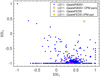 |
Fig. 11 eROSITA hardness ratios of LG11-Gaia M dwarfs detected in eFEDS (filled pink diamonds) and in eRASS1 (filled blue squares); see text in Sect. 6.5 for the definition of the hardness ratios. We show the CPM pairs in eFEDS and in eRASS1 samples in yellow. |
6.6.1 Comparison between eFEDS and eRASS1
We found that six LG11-Gaia M dwarfs are detected with eROSITA during eFEDS and eRASS1. We used the Lx values calculated in Sects. 4.1 and 5.1 for eFEDS and eRASS1 stars, respectively.
In Fig. 12 we show the comparison between the observed X-ray luminosities during the two different eROSITA epochs. Two stars showed Lx higher by a factor of two during eRASS1 than during eFEDS. From the eFEDS light curves in Fig. D.1, we know that PM I09201+0347 was detected during a flare. Therefore, the fact that the star was on average brighter during eRASS1 indicates that likely another, brighter flare occurred during the all-sky survey. A flare during eRASS1 is also a probable explanation for the change in X-ray luminosity of the other star, PM I08551+0132. In a future work, we will examine the X-ray variability of M dwarfs during eRASS in detail.
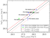 |
Fig. 12 Comparison between X-ray luminosities observed during eFEDS (log Lx,eFEDs) and eRASS1 (log Lx,eRAss1). Lx,eRAss1 is more than twice higher than Lx,eFEDS for the two stars above the dashed red line. |
6.6.2 Comparison between eROSITA and ROSAT
For the comparison on longer (decades) timescales, we cross-matched the LG11-Gaia/eFEDS and LG11-Gaia/eRASS1 samples with the ROSAT catalogs after correcting their Gaia-DR2 coordinates with the proper motions to the mean RASS epoch (January 1991). Following our conservative approach, we used a search radius of 30″ which is somewhat smaller than the values applied in other works on RASS data (e.g., Neuhaeuser et al. 1995). We found five stars from the LG11-Gaia/eFEDS sample and 340 from the LG11-Gaia/eRASS1 sample in the Second ROSAT All-Sky Survey Point Source Catalog (2RXS; Boller et al. 2016). We converted the count rates listed in the ROSAT catalogs into flux by adopting the ROSAT conversion factor from (Magaudda et al. 2020) (CF = 5.77 x 10⁻¹² erg cm−2 cnt−1). From the fluxes and distances, we then computed the X-ray luminosities observed with ROSAT (logLx,ROsAT), which refer to the 0.1–2.4 keV energy band. These values are presented in Table 5.
In Fig. 13 we show the comparison between Lx,eROSITA and Lx,ROSAT. We note again that this comparison is not affected by the different energy bands used for data from the two instruments. We find that 12 stars have Lx,eROSITA > 2 Lx,ROSAT and 53 stars have Lx,eROSITA < 0.5 Lx,ROSAT. All these variations are significant, that is, the error bars do not reach to the 1:1 line. It is striking that the X-ray luminosities in Fig. 13 are distributed symmetrically around the 1:1 line for log Lx [erg s−1] > 28, but the distribution shows an upward curvature for lower luminosities. eROSITA has a higher sensitivity than the RASS. The flux limit of eRASS1 is a factor 2–10 fainter than that of the 2RXS catalog; see values given by (Boller et al. 2016) and (Predehl et al. 2021). Therefore, the stars at the eROSITA detection limit are expected to be undetected during RASS, unless they were in a higher activity state (e.g., a flare) during the ROSAT survey. This is a likely explanation for the observation that at the faint end the ROSAT luminosities are higher than those measured by eROSITA.
In order to quantify the systematic deviation between the brightness seen in eROSITA and RASS for low-luminosity sources, we grouped log(Lx,eROSITA) with a bin size of 0.5 and calculated the mean of the ratio of the luminosities observed with eROSITA and with ROSAT for each bin, 〈 Lx,eROSITA/Lx,ROSAT〉bin. In the bottom panel of Fig. 13 we show the result of this statistical test, indicating the bin width (horizontal green lines), the number of stars in each bin (label at the tops of each data point), and the standard deviation of the mean of Lx,eROSITA/Lx,ROSAT in each bin as error bars. This ratio becomes increasingly lower for lower Lx, and it is significantly lower than one at the faint end. This systematic trend supports our above interpretation as an effect of sensitivity limits combined with intrinsic source variability.
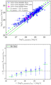 |
Fig. 13 Comparison between the X-ray luminosities from eROSITA (eRASS1 and eFEDS) and those from ROSAT (RASS) for the LG11-Gaia sample. Top panel: scatter plot. CPM pairs are highlighted in yellow. Bottom panel: ratio of the eROSITA and ROSAT luminosities in logarithmic bins of width 0.5 in X-ray luminosity, quantifying the systematic trend. Labels at the tops of the data points represent the number of stars in each bin. The vertical bars are the standard deviations, and the horizontal bars denote the bin width. |
7 Conclusions and outlook
We presented a comprehensive study of the X-ray activity of M dwarfs and its relation with stellar rotation. The careful match of our input target list, the proper motion catalog by (Lépine & Gaidos 2011), with Gaia DR2 data provides more reliable stellar parameters for these stars than the values used in previous studies on the same argument. Of the ~8300 nearby M dwarfs from this LG11-Gaia catalog,~8% have an X-ray detection in the first eROSITA All-Sky survey, and this X-ray sample is skewed to nearby stars (with a peak in their distance distribution at -20 pc). A subset of only about 1 out of 4 of the eROSITA-detected M dwarfs have detectable rotation periods in TESS light curves. We can therefore state that eROSITA X-ray measurements are a much more sensitive diagnostic for magnetic activity than star spot amplitudes measured with TESS.
From an eROSITA survey of the CalPV phase (the so-called eFEDS fields), we derived the first coronal luminosities and temperatures for M dwarfs obtained from eROSITA X-ray spectra. The resulting rate-to-flux conversion factor was the basis for the X-ray luminosities we determined for the faint majority of our sample stars, and the same CF can be used in future eROSITA studies of faint M dwarfs.
We examined the mass dependence of M dwarf X-ray activity on an unprecedentedly large sample, and we quantified its slope  , which is considerably steeper than the slope measured for the pre-main-sequence stars from the ONC study of (Preibisch et al. 2005) (βonc = 1.4), and it is offset toward lower luminosities by a factor that depends on the mass, that is, on the 2.0 logarithmic dex for
  and 0.8 dex for
  For a given mass, our validated M dwarfs display a spread in Lx of 0.6 decades. The true scatter is likely significantly larger because of the incompleteness of eRASS1 and eFEDS related to the flux limit discussed above.
The most obvious candidate for explaining the broad range of X-ray activity levels for a given M dwarf mass is a distribution of rotation periods (and ensuing dynamo efficiency). Our X-ray selected sample in the validated M dwarf mass range presents periods between 0.10 and 8.35 d, where the upper boundary is mostly produced by the duration of the TESS campaigns (~27 d). The possible influence of the flux limit of eROSITA on the Prot distribution of the sample can be examined in a direct study of the activity-rotation relation. We found that in the saturated regime, which by coincidence reaches roughly up to our period boundary of ~10 d, the eROSITA data comprise some stars with very faint X-ray emission  These are downward outliers in the saturated part of the rotation-activity relation, and their origin needs further investigation. On the basis of their log
  values, we might conjecture that eRASS can reach into the bulk of the stars in the unsaturated regime of slow rotators, but that facilities capable of providing longer periods must be used to detect their corresponding rotation signal.
With respect to ROSAT, even the first all-sky survey of eROSITA reaches lower X-ray activity levels, as we showed in our direct comparison of RASS and eRASS1 luminosities for the 345 M dwarfs that are detected in both surveys. These stars are about half of the eRASS1 sample. The majority of the other half that is not detected in RASS is near the eRASS1 detection limit (with ML_CTS_0≲ 20). Adding data from the other seven eROSITA surveys will provide access to X-ray detections of more and fainter M dwarfs in the near future.
Similarly, significant quantitative progress can be expected in our understanding of the coronal temperature distribution in M dwarfs, for which no statistical samples are available so far. Our results from the spectral analysis of about a dozen X-ray bright M dwarfs in eFEDS combined with the eROSITA hardness ratios for the full (but mostly faint) X-ray detected sample has shown that at least two-thirds of the eROSITA-detected M dwarfs have typical coronal temperatures of ~0.5 keV (corresponding to ~6MK). Our analysis of eROSITA/eFEDS spectra also shows that the relation between Lx and Tx of M dwarfs is poorly known so far. The huge number of relatively bright X-ray emitters in eRASS may place new constraints on this, however.
Finally, eROSITA has opened a new window for variability studies of coronal X-ray emission. Our comparison with RASS data has confirmed the evidence from previous much smaller samples of M dwarfs (e.g., Marino et al. 2000) that large changes of the X-ray luminosity are rare. Specifically, only 17% of our combined eROSITA/RASS sample displays variability by more than a factor of two between the two surveys. Because the most obvious candidates for X-ray variability in M dwarfs are flares, this low-variability amplitude clearly arises from the averaging over survey exposures (typically 6–8 intervals of ~40 s duration each and separated by ~4 h in case of eRASS). About one-third of the 14 M dwarfs detected in the eFEDS have significantly variable eROSITA light curves. Detailed studies of these short-term light curves are required to extract better estimates for the brightness scale of the variations. Moreover, the huge number of these light curves that is available with eROSITA should enable placing limits on the flare frequency of M dwarfs in the X-ray domain for the first time.
Acknowledgements
E.M. is supported by the Bundesministerium für Wirtschaft und Energie through the Deutsches Zentrum für Luft- und Raumfahrt e.V. (DLR) under grant number FKZ 50 OR 1808. A.K. is supported by the Deutsche Forschungsgemeinschaft (DFG) project number 413113723. J.W. is supported by the Deutsche Forschungsgemeinschaft (DFG, German Research Foundation) under Germany’s Excellence Strategy - EXC-2094-390783311. This work is based on data from eROSITA, the soft X-ray instrument aboard SRG, a joint Russian-German science mission supported by the Russian Space Agency (Roskosmos), in the interests of the Russian Academy of Sciences represented by its Space Research Institute (IKI), and the Deutsches Zentrum für Luft-und Raumfahrt (DLR). The SRG spacecraft was built by Lavochkin Association (NPOL) and its subcontractors, and is operated by NPOL with support from the Max Planck Institute for Extraterrestrial Physics (MPE). The development and construction of the eROSITA X-ray instrument was led by MPE, with contributions from the Dr. Karl Remeis Observatory Bamberg and ECAP (FAU Erlangen-Nuernberg), the University of Hamburg Observatory, the Leibniz Institute for Astrophysics Potsdam (AIP), and the Institute for Astronomy and Astrophysics of the University of Tübingen, with the support of DLR and the Max Planck Society. The Argelander Institute for Astronomy of the University of Bonn and the Ludwig Maximilians Universität Munich also participated in the science preparation for eROSITA. The eROSITA data shown here were processed using the eSASS/NRTA software system developed by the German eROSITA consortium. This paper includes data collected with the TESS mission, obtained from the MAST data archive at the Space Telescope Science Institute (STScI). Funding for the TESS mission is provided by the NASA Explorer Program. STScI is operated by the Association of Universities for Research in Astronomy, Inc., under NASA contract NAS 5–26555. This work has made use of data from the European Space Agency (ESA) mission Gaia (https://www.cosmos.esa.int/gaia), processed by the Gaia Data Processing and Analysis Consortium (DPAC, https://www.cosmos.esa.int/web/gaia/dpac/consortium). Funding for the DPAC has been provided by national institutions, in particular the institutions participating in the Gaia Multilateral Agreement. This publication makes use of data products from the Two Micron All Sky Survey, which is a joint project of the University of Massachusetts and the Infrared Processing and Analysis Center/California Institute of Technology, funded by the National Aeronautics and Space Administration and the National Science Foundation and of data products from the Wide-field Infrared Survey Explorer, which is a joint project of the University of California, Los Angeles, and the Jet Propulsion Laboratory/California Institute of Technology, funded by the National Aeronautics and Space Administration.
Appendix A Identification of Gaia DR2 counterparts to the M dwarfs from LG11
We matched the LG11 catalog with the second data release of the Gaia mission (Gaia DR2, Gaia Collaboration 2018b) using the proper motions (P.M.) given in LG11 to correct the epoch 2000 coordinates provided in the LG11 catalog to the Gaia epoch (J2015.5). Then we performed a multicone search with a search radius of 3″ around each target in LG11 with TOPCAT (Taylor 2005). In this step, we found 9638 Gaia entries for the 8889 LG11 stars, 736 of which have multiple matches (723 doubles and 13 triples). To identify reliable Gaia counterparts and to avoid sources in the search radius that do not belong to our targets (i.e., that are no companions to our targets), we used two additional criteria.
Firstly, we calculated for all Gaia entries in our matched catalog the total Gaia P.M. by taking the square root of the quadratic sum of the proper motions in right ascension and in declination. Then we computed the difference between the total LG11 proper motion and the total Gaia proper motion. The histogram of this proper motion difference shows a Gaussian shape with a sharp edge at +0.2″/yr when only the stars with a single Gaia match are considered. Therefore, we removed all Gaia counterparts from the full list that show a proper motion difference outside this range. This criterion reduced our catalog to 8779 entries, 440 of which show multiple Gaia matches. During this step, all stars without proper motions given in Gaia DR2 were also removed. As a second step, we converted the Gaia magnitudes into J-band magnitudes (which we call JGaia) using the relation given on the ESA webpage6. Then we calculated the difference between the Two Micron All-Sky Survey (2MASS; Skrutskie et al. 2006) J-band magnitude listed in the LG11 catalog and JGaia. Significant differences between these magnitudes can arise when two adjacent Gaia sources are not resolved in 2MASS. The two Gaia sources often form a common proper motion (CPM) pair. Therefore, to keep in our catalog the CPM pairs with a moderate J-band magnitude difference that are potentially composed of two M stars, we removed all Gaia counterparts with JGaia—J > ±2mag. After this removal of wrong identifications and faint companions that are not relevant as a potential X-ray source, the catalog contained 8489 entries, 169 of which still show multiple Gaia matches. We note that in this step, all Gaia counterparts without magnitudes in Gaia DR2 were removed as well. The 169 multiple matches were checked through inspection by eye using ESASky7 (Merín et al. 2017), and 150 of them were found to be comoving pairs.
After the application of our selection criteria, 571 LG11 stars were found to have no Gaia counterpart, either because their Gaia data are missing or incomplete, that is, no proper motions and/or no magnitudes are available in DR2. These stars were removed during the cleaning process described above. To recover the Gaia IDs for the targets with incomplete data, our initial 3″ multicone match was repeated for these 571 stars. We found that 414 of them have Gaia matches (but with incomplete photometric and/or astrometric information), and 33 of them have multiple Gaia sources in the search radius. The multiple matches were again checked with an inspection by eye, and we found that 30 of them are CPM pairs. As a final check for our match, we used the cross-identification function of the SIMBAD astronomical database (Wenger et al. 2000). We uploaded the list of target names from LG11 and converted them into Gaia DR2 SOURCE_ID. The results of our match procedure explained in the previous paragraphs and the output from SIMBAD were compared, and if they were not consistent, an inspection by eye was applied. (SIMBAD does not always provide the correct Gaia ID for a given target, which is why we performed the match procedure described above).
As the final result, we found 8917 Gaia counterparts for 8736 targets from the LG11 catalog. Gaia data are not available for the remaining 153 LG11 targets. The excess of Gaia counterparts represents the 180 stars for which we found common proper motion companions of |∆J| ≤ 2 mag, one of which is a triple system. These objects add to the binary stars that are listed as resolved pairs in the original LG11 catalog (104 binary pairs). Because the CPM companions discovered through our match of the LG11 catalog with Gaia DR2 were added to our table, the total number of objects in our target list is 9070 (8917 stars with Gaia counterparts, including the CPM companions and 153 stars without a Gaia counterpart).
Appendix B Independent cross-check of the source identification with NWAY
To examine the reliability of our position-based source identification procedure, we took advantage of the catalogs of counterparts for eFEDS and eRASS1 identified within the eROSITA_DE collaboration. For eFEDS, we used the catalog presented by (Salvato et al. 2022), where NWAY (Salvato et al. 2018) and ASTROMATCH (Ruiz et al. 2018) algorithms were applied and tested. They found an agreement for 88 % in the counterpart identification, with NWAY having higher completeness and purity (above 96 %). In this catalog, less than 1 % of the sources have a secure counterpart identified only by ASTRO-MATCH. For this reason, we speak here only of NWAY. For eRASS1, we used a preliminary catalog of counterparts that were obtained with NWAY, ran with the same photometric priors and astrometric setup as for eFEDS. The counterparts were identified using the photometry provided in LS8, where images were calibrated to Gaia-DR2 and photometry was obtained in g, r, and z bands from the three individual imaging surveys. In addition, the photometry was forced at the optical positions on unWISE maps for all sources detected in the combined grz image using the TRACTOR algorithm from (Lang 2014). For the bright sources, the catalog lists the Gaia-DR2 properties.
B.1 eFEDS
For eFEDS, we checked the counterparts of the 14 X-ray sources that we associated with a LG11-Gaia M dwarf. The match with the eFEDS NWAY catalog through the eROSITA unique source identification shows that 12 of them have assigned the same Gaia counterpart. The other 2 do not have a Gaia source ID in the NWAY catalog for eFEDS source counterparts, but a simple cross-match in coordinates indicates a separation of less than - 0.01″ between our counterparts and those listed in (Salvato et al. 2022), clearly demonstrating that these are indeed the same sources. The failure to identify the Gaia CTP upon construction of the NWAY catalog is due to the high P.M. of these two stars.
B.2 eRASS1
For eRASS1, we examined the 842 X-ray sources identified by us with an LG11-Gaia star in the first step of our identification procedure (see Sect. 3.2). We recall that our final list LG11-Gaia/eRASS1 comprises only 673 stars, a subsample of these 842.
LS8 did not completely cover the eRASS1, and for this reason, the comparison can be made only for 382 sources. Among these 382 eRASS1 sources, 347 are associated in NWAY-LS8 with the same Gaia-ID that we found as closest CTP to the eRASS1 source, but 21 out of 347 are not our LG11-Gaia stars, and we have disregarded them in our final catalog after the reverse match. Of the remaining 35 eRASS1 sources that are present in NWAY-LS8, five have a nonzero probability according to NWAY-LS8 for more than one optical counterpart to be associated with this eROSITA source. For all of them, the LG11-Gaia star is one of the possible counterparts. Moreover, NWAY-LS8 assings a different Gaia source to 19 objects (i.e., not our closest CTP) as the most likely CTP, and the NWAY-LS8 counterpart for the remainder (11 objects) is not matched to a Gaia-DR2 source.
It is important to consider that in the current version of the NWAY-LS8 catalog of the eRASS1 counterparts, no attempt was made to correct the coordinates of the sources for proper motion. This biasing the results specifically against the type of sources that are presented in this paper. Therefore, we investigated the 11 objects without Gaia-ID in NWAY-LS8 through visual inspection on ESASky, finding that the LG11-Gaia star is indeed the best CTP for all. For example because its P.M. points towards the eRASS1 position or because there is no other optical/NIR bright object nearby. The lack of a CTP in NWAY probably arises because of the high P.M. of the stars.
For the remaining 19 objects to which NWAY associates a different CTP with the eRASS1 source than we did, NWAY-LS8 chose the LG11-Gaia star for 11, while we excluded these stars from our final sample based on our reverse match, which showed that they are not the closest CTP to the X-ray position. Another 3 are part of CPM systems for which NWAY-LS8 chose the Gaia ID of the companion, and for one, neither the object selected with NWAY nor the LG11-Gala star is the closest CTP to the eRASS1 source. For the 4 remaining eRASS1 sources, we disagree with NWAY-LS8, which does not consider the LG11-Gaia M dwarf as the best association, although it is the closest CTP.
To summarize, of the 842 eRASS1 sources with a LG11-Gaia star in our 15″ search radius, we were able to compare 382 with NWAY-LS8. NWAY-LS8 disagrees with our results for the counterpart for 1 % of X-ray sources that we associate with a LG11-Gaia M dwarf (4 out of 382). On the other hand, according to NWAY-LS8, we incorrectly discarded 3 % of the LG11-Gaia stars (11 out of 382) in our reverse match because they are not the closest counterpart to the X-ray position. NWAY-LS8 missed 3 % (11 cases) of the LG11-Gaia stars because the input catalog adopted for the identification of the counterpart did not correct the coordinates of the moving sources for proper motion. To conclude, the two methods of source identification agree for 93 % of the objects.
Appendix C Best-fit spectral model
Fig. C.1 displays the eROSITA spectra from the eFEDS observation for the ten brightest M dwarfs in the field, as discussed in Sect. 4.1.2. The best-fitting model from Table 4 is overlaid, and the bottom panels show the residuals between data and model.
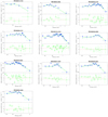 |
Fig. C1 eROSITA spectrum, best-fit thermal model, and residuals for the ten sources in the eFEDS fields with > 30 counts. |
Appendix D eFEDS light curves
Fig. D.1 comprises the eROSITA light curves from the eFEDS observation for the 14 detected M dwarfs in these fields. The timing of the data intervals in these light curves is a consequence of the survey mode employed in the data acquisition for the eFEDS fields and is described in Sect. 4.1.3.
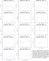 |
Fig. D.1 eROSITA light curves for the 14 M dwarfs detected in the eFEDS fields. The bin size (given above each panel) was individually adapted taking the sampling of the light curve into account that resulted from the scanning mode, which was chosen such as to produce the smallest error bars; see text in Sect. 4.1.3 for details. |
References
- An, D., Terndrup, D. M., Pinsonneault, M. H., et al. 2007, ApJ, 655, 233 [NASA ADS] [CrossRef] [Google Scholar]
- Bailer-Jones, C. A. L., Rybizki, J., Fouesneau, M., Mantelet, G., & Andrae, R. 2018, AJ, 156, 58 [Google Scholar]
- Bertin, E., & Arnouts, S. 1996, A&AS, 117, 393 [NASA ADS] [CrossRef] [EDP Sciences] [Google Scholar]
- Boller, T., Freyberg, M. J., Trümper, J., et al. 2016, A&A, 588, A103 [NASA ADS] [CrossRef] [EDP Sciences] [Google Scholar]
- Boller, T., Schmitt, J. H. M. M., Buchner, J., et al. 2022, A&A, 661, A8 (eROSITA EDR SI) [NASA ADS] [CrossRef] [EDP Sciences] [Google Scholar]
- Broeg, C., Fernández, M., & Neuhäuser, R. 2005, Astron. Nachr., 326, 134 [NASA ADS] [CrossRef] [Google Scholar]
- Brunner, H., Liu, T., Lamer, G., et al. 2022, A&A, 661, A1 (eROSITA EDR SI) [NASA ADS] [CrossRef] [EDP Sciences] [Google Scholar]
- Choi, P. I., & Herbst, W. 1996, AJ, 111, 283 [NASA ADS] [CrossRef] [Google Scholar]
- Dey, A., Schlegel, D. J., Lang, D., et al. 2019, AJ, 157, 168 [Google Scholar]
- Favata, F., Reale, F., Micela, G., et al. 2000, A&A, 353, 987 [NASA ADS] [Google Scholar]
- Feinstein, A. D., Montet, B. T., Foreman-Mackey, D., et al. 2019, PASP, 131, 094502 [Google Scholar]
- Fleming, T. A. 1998, ApJ, 504, 461 [NASA ADS] [CrossRef] [Google Scholar]
- Fleming, T., & Stone, J. M. 2003, ApJ, 585, 908 [NASA ADS] [CrossRef] [Google Scholar]
- Fleming, T. A., Liebert, J., Gioia, I. M., & Maccacaro, T. 1988, ApJ, 331, 958 [NASA ADS] [CrossRef] [Google Scholar]
- Foster, G., Poppenhaeger, K., Ilic, N., & Schwope, A. 2022, A&A, 661, A23 (eROSITA EDR SI) [NASA ADS] [CrossRef] [EDP Sciences] [Google Scholar]
- Gaia Collaboration (Prusti, T., et al.) 2016, A&A, 595, A1 [NASA ADS] [CrossRef] [EDP Sciences] [Google Scholar]
- Gaia Collaboration (Babusiaux, C., et al.) 2018a, A&A, 616, A10 [NASA ADS] [CrossRef] [EDP Sciences] [Google Scholar]
- Gaia Collaboration (Brown, A. G. A., et al.) 2018b, A&A, 616, A1 [NASA ADS] [CrossRef] [EDP Sciences] [Google Scholar]
- Gilliland, R. L., & Fisher, R. 1985, PASP, 97, 285 [CrossRef] [Google Scholar]
- Johnstone, C. P., & Güdel, M. 2015, A&A, 578, A129 [NASA ADS] [CrossRef] [EDP Sciences] [Google Scholar]
- Lang, D. 2014, AJ, 147, 108 [Google Scholar]
- Lépine, S., & Gaidos, E. 2011, AJ, 142, 138 [Google Scholar]
- Lindegren, L., Hernández, J., Bombrun, A., et al. 2018, A&A, 616, A2 [NASA ADS] [CrossRef] [EDP Sciences] [Google Scholar]
- Magaudda, E., Stelzer, B., Covey, K. R., et al. 2020, A&A, 638, A20 [NASA ADS] [CrossRef] [EDP Sciences] [Google Scholar]
- Maggio, A., Flaccomio, E., Favata, F., et al. 2007, ApJ, 660, 1462 [NASA ADS] [CrossRef] [Google Scholar]
- Mann, A. W., Feiden, G. A., Gaidos, E., Boyajian, T., & von Braun, K. 2015, ApJ, 804, 64 [Google Scholar]
- Mann, A. W., Feiden, G. A., Gaidos, E., Boyajian, T., & von Braun, K. 2016, ApJ, 819, 87 [NASA ADS] [CrossRef] [Google Scholar]
- Marino, A., Micela, G., & Peres, G. 2000, A&A, 353, 177 [NASA ADS] [Google Scholar]
- Matt, S. P., Brun, A. S., Baraffe, I., Bouvier, J., & Chabrier, G. 2015, ApJ, 799, L23 [Google Scholar]
- McQuillan, A., Mazeh, T., & Aigrain, S. 2013, ApJ, 775, L11 [Google Scholar]
- McQuillan, A., Mazeh, T., & Aigrain, S. 2014, ApJS, 211, 24 [Google Scholar]
- Merín, B., Salgado, J., Giordano, F., et al. 2017, ASP Conf. Ser., 512, 495 [Google Scholar]
- Modirrousta-Galian, D., Stelzer, B., Magaudda, E., et al. 2020, A&A, 641, A113 [NASA ADS] [CrossRef] [EDP Sciences] [Google Scholar]
- Neuhaeuser, R., Sterzik, M. F., Schmitt, J. H. M. M., Wichmann, R., & Krautter, J. 1995, A&A, 297, 391 [NASA ADS] [Google Scholar]
- Newton, E. R., Irwin, J., Charbonneau, D., Berta-Thompson, Z. K., & Dittmann, J. A. 2016, ApJ, 821, L19 [NASA ADS] [CrossRef] [Google Scholar]
- Newton, E. R., Irwin, J., Charbonneau, D., et al. 2017, ApJ, 834, 85 [Google Scholar]
- Pallavicini, R., Golub, L., Rosner, R., et al. 1981, ApJ, 248, 279 [NASA ADS] [CrossRef] [Google Scholar]
- Parker, E. N. 1993, ApJ, 408, 707 [NASA ADS] [CrossRef] [Google Scholar]
- Pizzolato, N., Maggio, A., Micela, G., Sciortino, S., & Ventura, P. 2003, Ar&A, 397, 147 [Google Scholar]
- Predehl, P., Andritschke, R., Arefiev, V., et al. 2021, A&A, 647, A1 [EDP Sciences] [Google Scholar]
- Preibisch, T., & Feigelson, E. D. 2005, ApJS, 160, 390 [NASA ADS] [CrossRef] [Google Scholar]
- Preibisch, T., Kim, Y.-C., Favata, F., et al. 2005, ApJS, 160, 401 [NASA ADS] [CrossRef] [Google Scholar]
- Raetz, S., Schmidt, T. O. B., Czesla, S., et al. 2016, MNRAS, 460, 2834 [NASA ADS] [CrossRef] [Google Scholar]
- Raetz, S., Stelzer, B., Damasso, M., & Scholz, A. 2020, A&A, 637, A22 [NASA ADS] [CrossRef] [EDP Sciences] [Google Scholar]
- Reiners, A., Joshi, N., & Goldman, B. 2012, AJ, 143, 93 [Google Scholar]
- Reiners, A., Schüssler, M., & Passegger, V. M. 2014, ApJ, 794, 144 [Google Scholar]
- Ribas, I., Bolmont, E., Selsis, F., et al. 2016, A&A, 596, A111 [NASA ADS] [CrossRef] [EDP Sciences] [Google Scholar]
- Ricker, G. R., Winn, J. N., Vanderspek, R., et al. 2014, SPIE Conf. Ser., 9143, 914320 [Google Scholar]
- Robrade, J., & Schmitt, J. H. M. M. 2005, A&A, 435, 1073 [NASA ADS] [CrossRef] [EDP Sciences] [Google Scholar]
- Robrade, J., Poppenhaeger, K., & Schmitt, J. H. M. M. 2010, A&A, 513, A12 [NASA ADS] [CrossRef] [EDP Sciences] [Google Scholar]
- Rodríguez-Ledesma, M. V., Mundt, R., & Eislöffel, J. 2009, A&A, 502, 883 [NASA ADS] [CrossRef] [EDP Sciences] [Google Scholar]
- Rosen, S. 2016, VizieR Online Data Catalog: IX/47 [Google Scholar]
- Rosner, R., Golub, L., & Vaiana, G. S. 1985, ARA&A, 23, 413 [NASA ADS] [CrossRef] [Google Scholar]
- Ruiz, A., Corral, A., Mountrichas, G., & Georgantopoulos, I. 2018, A&A, 618, A52 [NASA ADS] [CrossRef] [EDP Sciences] [Google Scholar]
- Salvato, M., Buchner, J., Budavári, T., et al. 2018, MNRAS, 473, 4937 [Google Scholar]
- Salvato, M., Wolf, J., Dwelly, T., et al. 2022, A&A, 661, A3 (eROSITA EDR SI) [NASA ADS] [CrossRef] [EDP Sciences] [Google Scholar]
- Schmitt, J. H. M. M., & Liefke, C. 2004, A&A, 417, 651 [NASA ADS] [CrossRef] [EDP Sciences] [Google Scholar]
- Shu, Y., Koposov, S. E., Evans, N. W., et al. 2019, MNRAS, 489, 4741 [Google Scholar]
- Skrutskie, M. F., Cutri, R. M., Stiening, R., et al. 2006, AJ, 131, 1163 [NASA ADS] [CrossRef] [Google Scholar]
- Stelzer, B., Marino, A., Micela, G., López-Santiago, J., & Liefke, C. 2013, MNRAS, 431, 2063 [Google Scholar]
- Stelzer, B., Damasso, M., Scholz, A., & Matt, S. P. 2016, MNRAS, 463, 1844 [NASA ADS] [CrossRef] [Google Scholar]
- Stelzer, B., Klutsch, A., Coffaro, M., Magaudda, E., & Salvato, M. 2022, A&A, 661, A44 (eROSITA EDR SI) [NASA ADS] [CrossRef] [EDP Sciences] [Google Scholar]
- Tarter, J. C., Backus, P. R., Mancinelli, R. L., et al. 2007, Astrobiology, 7, 30 [NASA ADS] [CrossRef] [Google Scholar]
- Taylor, M. B. 2005, ASP Conf. Ser., 347, 29 [Google Scholar]
- Thompson, S. E., Fraquelli, D., Van Cleve, J. E., & Caldwell, D. A. 2016, Kepler Archive Manual, Kepler Science Document KDMC-10008-006 [Google Scholar]
- Tu, L., Johnstone, C. P., Güdel, M., & Lammer, H. 2015, A&A, 577, L3 [NASA ADS] [CrossRef] [EDP Sciences] [Google Scholar]
- van den Besselaar, E. J. M., Raassen, A. J. J., Mewe, R., et al. 2003, A&A, 411, 587 [NASA ADS] [CrossRef] [EDP Sciences] [Google Scholar]
- Wenger, M., Ochsenbein, F., Egret, D., et al. 2000, A&AS, 143, 9 [NASA ADS] [CrossRef] [EDP Sciences] [Google Scholar]
- West, A. A., Weisenburger, K. L., Irwin, J., et al. 2015, ApJ, 812, r3 [NASA ADS] [CrossRef] [Google Scholar]
- Wright, N. J., & Drake, J. J. 2016, Nature, 535, 526 [Google Scholar]
- Wright, N. J., Drake, J. J., Mamajek, E. E., & Henry, G. W. 2011, ApJ, 743, 48 [Google Scholar]
- Wright, N. J., Newton, E. R., Williams, P. K., Drake, J. J., & Yadav, R. K. 2018, MNRAS, 479, 2351 [NASA ADS] [CrossRef] [Google Scholar]
- Zechmeister, M., & Kürster, M. 2009, A&A, 496, 577 [CrossRef] [EDP Sciences] [Google Scholar]
The table A Modern Mean Dwarf Stellar Color and Effective Temperature Sequence is maintained by E. Mamajek at http://www.pas.rochester.edu/~emamajek/EEM_dwarf_UBVIJHK_colors_Teff.txt
XSPEC NASA's HEASARC Software: https://heasarc.gsfc.nasa.gov/xanadu/xspec/ Article number, page 8 of 23
More information about APEC model used by XSPEC software can be found at https://heasarc.gsfc.nasa.gov/xanadu/xspec/manual/node135.html
Fortran Version v2.3.01 released: 2011-09-13 by Mathias Zechmeister.
All Tables
X-ray spectral parameters for the ten M stars in eFEDS with more than 30 counts in the 0.2–5.0 keV band.
Measurements of X-ray activity and rotation derived by us from eROSITA, ROSAT, and TESS data.
Results obtained from fitting Lx – M⋆ and L/Lbol – M⋆ for the full sample (LG11-Gaia-eFEDS, LG11-Gaia-eRASS1 and Gaia-Magaudda20) and for the saturated subsamples, i.e., stars with Prot ≤ Psat; see Sects. 6.2 and 6.3 for details.
All Figures
|
Fig. 1 Gaia CMD based on DR2 data for the LG11 sample with Gaia distance and photometry. The pink line represents the main sequence by E. Mamajek (see footnote 1). A residual contamination by giant stars is present. Stars with MG > 5 mag and MKs > 4.6 (the magnitude above which the polynomial relations between photometry and stellar parameters of (Mann et al. 2015) are valid) are highlighted in green. |
| In the text | |
|
Fig. 2 Distance distributions (dBJ18) for various subsamples of the LG11 catalog according to our match with Gaia DR2. Left: giant stars (in gray) and main-sequence stars (in red). Right: zoom into the main-sequence sample (red) and subsample of validated main-sequence stars (green). See text in Sect. 3. |
| In the text | |
|
Fig. 3 Distribution of Gaia distances from (Bailer-Jones et al. 2018) and spectral types calculated from Gbp – Grp. Top panel: gray histogram is the distribution for the stars from LG11-Gaia in the eFEDS fields. The green contours represent the distance and SpT distribution for those stars observed by TESS. We show the CPM pairs in yellow. Bottom panel: stars from the LG11-Gaia sample identified in the preliminary eRASS1 catalog. For simplicity, we do not show the four CPM pairs here because they represent only 4% of the sample. |
| In the text | |
|
Fig. 4 Separation between the X-ray to optical positions for the 842 direct matches of LG11-Gaia stars with the eRASS1 catalog. All 2148 possible Gaia-DR2 CTPs found with the reverse match within 15” are shown in gray. The same objects after the application of their P.M. correction are plotted in green. The red histogram represents the Gaia-DR2 CTP that is closest to each eRASS1 source of our sample, the 734 closest CTPs that correspond to the LG11-Gaia stars studied in this work are shown in blue, and the final LG11-Gaia/eRASS1 sample of 673 M dwarfs is shown in black. |
| In the text | |
|
Fig. 5 X-ray-to-optical flux ratio vs. Gaia color for the closest optical counterparts to the X-ray sources selected from the match of LG11-Gaia with the eRASS1 catalog. Two distinct regions are visible: the extra-galactic area with high log(fx/fG) values and relatively blue Gaia color, and the star region with lower values of log(fx/fG) and redder Gaia color, separated by the dashed black line we derived from Fig. B3 in Stelzer et al. 2022). The filled red squares are the 673 eRASS1 sources that we identified as M dwarfs (see text in Sect. 3.2), and the filled yellow squares represent the four stars that have a comoving companion. We show only the sources with SepX,opt < 3 x RADEC_ERR. |
| In the text | |
|
Fig. 6 Comparison of the pipeline-produced PDCSAP light curve of PMI09034-0023 (TIC 893123, gray) and our own photometry (black) extracted from the full frame images. Within the error bars, the two light curves agree with each other, while the scatter is much larger for the light curve with the two-minute cadence. The shape of the light curve is different, however, which results in different estimates of the rotation period. |
| In the text | |
|
Fig. 7 X-ray activity and rotation vs. mass: blue and pink show the eRASS1 and eFEDS M dwarf samples, respectively, and gray shows the revised sample from (Magaudda et al. 2020); see the legend inside the panels for other literature data and highlighted specific subsamples. In the top panels, the median and the standard deviation of the data are presented in red for bins with a width of 0.1 M⊙. Top left: X-ray luminosity vs. mass and best fit (cyan). Top right: X-ray over bolometric luminosity vs. mass and best fit (cyan). Bottom left: rotation period vs mass; for the stars with double-humped TESS light curves, the shorter of the two periods is shown. |
| In the text | |
|
Fig. 8 X-ray activity-rotation relations. Left: X-ray luminosity vs rotation period with mass-color code in steps of 0.1 M⊙. Right: X-ray luminosity as a fraction of bolometric luminosity vs. Rossby number. See the legend, the caption of Fig. 7, and the text in Sect. 6.3 for the subsamples we display. |
| In the text | |
|
Fig. 9 X-ray activity vs mass for the validated samples (see legend in Figs. 7 and 8) restricted to the saturated stars, i.e., stars with Prot ≤ 8.5 d, best fit (violet) and median plus standard deviation of the data (red) in bins of 0.1 M⊙. The fit to the young stars in the Orion Nebular cluster provided by (Preibisch et al. 2005) is also shown, together with the standard deviation of this fit (green) and the best fit we found for the full M dwarf sample presented in the top panels of Fig. 7 (cyan). Left: X-ray luminosity vs. mass. Right: X-ray over bolometric luminosity vs. mass. |
| In the text | |
|
Fig. 10 Coronal temperature vs. X-ray luminosity for M dwarfs with eROSITA spectra (red circles), compared to FGKM stars from (Johnstone & Gudel 2015) (black circles) for which according to our updated analysis there are six M dwarfs (filled circles and individually labeled: 1 – AU Mic, 2 – EV Lac, 3 – AD Leo, 4 – YZ CMi, 5 – Prox Cen, and 6 – SCR 1845). Stars labeled low-mass (M⋆ ≤ 0.65 M⊙) in (Johnstone & Gudel 2015) but which have SpT K are marked with a cross. At the faint and cool end lies the planet-hosting M dwarf GJ 357 from (Modirrousta-Galian et al. 2020) (blue circle). |
| In the text | |
|
Fig. 11 eROSITA hardness ratios of LG11-Gaia M dwarfs detected in eFEDS (filled pink diamonds) and in eRASS1 (filled blue squares); see text in Sect. 6.5 for the definition of the hardness ratios. We show the CPM pairs in eFEDS and in eRASS1 samples in yellow. |
| In the text | |
|
Fig. 12 Comparison between X-ray luminosities observed during eFEDS (log Lx,eFEDs) and eRASS1 (log Lx,eRAss1). Lx,eRAss1 is more than twice higher than Lx,eFEDS for the two stars above the dashed red line. |
| In the text | |
|
Fig. 13 Comparison between the X-ray luminosities from eROSITA (eRASS1 and eFEDS) and those from ROSAT (RASS) for the LG11-Gaia sample. Top panel: scatter plot. CPM pairs are highlighted in yellow. Bottom panel: ratio of the eROSITA and ROSAT luminosities in logarithmic bins of width 0.5 in X-ray luminosity, quantifying the systematic trend. Labels at the tops of the data points represent the number of stars in each bin. The vertical bars are the standard deviations, and the horizontal bars denote the bin width. |
| In the text | |
|
Fig. C1 eROSITA spectrum, best-fit thermal model, and residuals for the ten sources in the eFEDS fields with > 30 counts. |
| In the text | |
|
Fig. D.1 eROSITA light curves for the 14 M dwarfs detected in the eFEDS fields. The bin size (given above each panel) was individually adapted taking the sampling of the light curve into account that resulted from the scanning mode, which was chosen such as to produce the smallest error bars; see text in Sect. 4.1.3 for details. |
| In the text | |
Current usage metrics show cumulative count of Article Views (full-text article views including HTML views, PDF and ePub downloads, according to the available data) and Abstracts Views on Vision4Press platform.
Data correspond to usage on the plateform after 2015. The current usage metrics is available 48-96 hours after online publication and is updated daily on week days.
Initial download of the metrics may take a while.