| Issue |
A&A
Volume 661, May 2022
The Early Data Release of eROSITA and Mikhail Pavlinsky ART-XC on the SRG mission
|
|
|---|---|---|
| Article Number | A19 | |
| Number of page(s) | 9 | |
| Section | Galactic structure, stellar clusters and populations | |
| DOI | https://doi.org/10.1051/0004-6361/202141024 | |
| Published online | 18 May 2022 | |
Spatially resolved X-ray spectra of the galactic SNR G18.95-1.1: SRG/eROSITA view
1
Ioffe Institute,
26 Politekhnicheskaya st.,
St. Petersburg 194021, Russia
e-mail: This email address is being protected from spambots. You need JavaScript enabled to view it.
; This email address is being protected from spambots. You need JavaScript enabled to view it.
2
Space Research Institute of the Russian Academy of Sciences (IKI),
84/32 Profsoyuznaya st.,
Moscow 117997, Russia
3
Max Planck Institute for Astrophysics,
Karl-Schwarzschild-Str. 1,
85741
Garching, Germany
e-mail: This email address is being protected from spambots. You need JavaScript enabled to view it.
Received:
8
April
2021
Accepted:
19
August
2021
Abstract
Aims. We study the X-ray emission of the galactic supernova remnant (SNR) G18.95-1.1 with the eROSITA telescope on board the Spectrum Röntgen Gamma (SRG) orbital observatory. In addition to the pulsar wind nebula that was previously identified and examined by ASCA and Chandra, we study the X-ray spectra of the bright SNR ridge, which is resolved into a few bright clumps.
Methods. The wide field of view and the large collecting area in the 0.2-2.3 keV energy range of SRG/eROSITA allowed us to perform spatially resolved spectroscopy of G18.95-1.1.
Results. The X-ray ridge of G18.95-1.1 is asymmetric, indicating either supernova ejecta asymmetry or their interaction with a cloud. The X-ray dim northern regions outside the pulsar wind nebula can be described by a thin thermal plasma emission with a temperature ~0.3keV and a solar composition. The X-ray spectra of a few bright clumps located along the southern ridge may be satisfactorily approximated by a single thermal component of the Si-rich ejecta at the collisional ionization equilibrium with a temperature of about 0.3 keV. The bright ridge can be alternatively fit with a single component that is not dominated by equilibrium ejecta with T ~ 0.6 keV. The high ratio of the derived Si/O abundances indicates that the ejecta originated in deep layers of the progenitor star. The plasma composition of a southern Si-rich clump and the bright ridge are similar to what was earlier found in the Vela shrapnel A and G.
Key words: ISM: supernova remnants / X-rays: individuals: SNR G18.95-1.1 / X-rays: ISM
© ESO 2022
1 Introduction
Supernova remnant (SNR) G18.95-1.1, which is located in the Galactic plane within the central radian of the Milky Way, was discovered by Fuerst et al. (1985) in the course of the 2.695 GHz Galactic plane survey (Reich et al. 1984). Later on, it was studied at other frequencies in the radio band by Odegard (1986), Barnes & Turtle (1988), Patnaik et al. (1988), Furst et al. (1989), Fuerst et al. (1997), Reich (2002), and Sun et al. (2011). The radio and X-ray observations revealed that G18.95-1.1 belongs to the class of the composite-type SNR with a central peak emission. The central emission region is dominated by a pulsar wind nebulae (PWN) that was studied with the Chandra X-ray Observatory (Tüllmann et al. 2010). In the optical, the Hα imaging of the G18.95-1.1 region was performed by Stupar & Parker (2011). In X-rays, G18.95-1.1 was observed with the ROSAT (Aschenbach et al. 1991; Fuerst et al. 1997), ASCA (Harrus et al. 2004), and Chandra (Tüllmann et al. 2010) orbital X-ray observatories. The γ-ray source FL8Y J1829.5-1254 in the Fermi-LAT catalog (Acero et al. 2016) may be associated with this supernova remnant.
The ROSAT X-ray spectrum of G18.95-1.1 was fit by Aschenbach et al. (1991) with an absorbed thermal emission model with NH = 3.4 × 1021 cm−2 and T = 0.434keV. Their analysis also revealed two other χ2-statistics minima (reduced χ2 < 1) with parameter values NH = 9.5 × 1021 cm−2, T = 0.2keV, and NH = 5.2 × 1020 cm−2, T = 1.1 keV, which where rejected. Fuerst et al. (1997) obtained a slightly different result with best-fit parameters values NH = 3.4 × 1021 cm−2, T = 0.95 keV (χ2/d.o.f. = 0.84), and Nh = 12.5 × 1021 cm−2, T = 0.25 keV (χ2/d.o.f. = 0.86). They adopted the lower value of NH = (3.4 ± 1.5) × 1021 cm−2, which is consistent within the 90% confidence level errors with the NH = (2.0–2.2) × 1021 cm−2 obtained from the HI radio observations (Fuerst et al. 1997). On the other hand, analyzing a joint fit of the ROSAT and ASCA spectra, Harrus et al. (2004) obtained higher values of NH for a few various plasma emission models: collisional ionization equilibrium (CIE), the thermal MEKAL (Mewe-Gronenschild-aastra) model by Mewe et al. (1985); Kaastra & Jansen (1993), and thermal emission with nonequilibrium ionization (NEI), the PSHOCK model by Borkowski et al. (2001). The best-fit model parameters were NH = 8.4 × 1021 cm−2, T = 0.58 keV for the CIE and NH = 9.4 × 1021 cm−2, T = 0.9 keV for the NEI models with solar abundances. However, for the single-component models, the reduced χ2 values were rather high (χ2/d.o.f. = 1.76, d.o.f. = 89 for NEI and χ2/d.o.f. = 3.15, d.o.f. = 90 for CIE models), which might be evidence that more complicated modls of the source emission are required that allow abundance variation or additional components. The distance estimates to SNR G18.95-1.1 were discussed in detail by Furst et al. (1989), Harrus et al. (2004), and Tüllmann et al. (2010). It was suggested that the most plausible distance is ~2 kpc, which agrees with the HI measurements by Furst et al. (1989). The higher NH value obtained from the X-ray spectral analysis might be explained when molecular H2 or dust are assumed to contribute substantially to absorption in the direction to G18.95-1.1. This is discussed in more detail at the end of Sect. 2.
Chandra observations of G18.95-1.1 by Tüllmann et al. (2010) were dedicated to study the PWN, and the Chandra field of view (FOV) only permitted studying its immediate surroundings. The temperature of the plasma emission component in the PWN region was found to be T = 0.48 keV, and the power-law component index was found to vary from 1.4 to 1.9, depending on the size of the considered emission region. The relatively hard power-law index and the elongated shape of the PWN may indicate that the bow shock-type nebula is produced by the interaction with the flow behind the reverse shock that passed through the PWN, as was proposed for the Vela PWN by Chevalier & Reynolds (2011) and Bykov et al. (2017).
The location of G18.95-1.1 in the inner galactic plane makes the spectral analysis rather difficult because of the uncertainty and inhomogeneity of the background radiation and the contamination by the emission from point sources projected at the SNR. The brightest X-ray point source is the ROSAT emission excess J182848-130055 discussed by Fuerst et al. (1997) and Harrus et al. (2004). In the ASCA map, this source is located at the position J182849.9-130107.44. Harrus et al. (2004) discussed the possible coincidence of this source with the star J182850.08-130120.3. Another point source is CXOU J182913.1-125113, which is located at the edge of the PWN region and is a pulsar candidate. However, it has no radio or optical counterpart (Tüllmann et al. 2010). There are also other point sources in the vicinity of the SNR. The Chandra observatory is ideally suited for identifying and excising the point sources, but its FOV covers only a small part of the G18.95-1.1 remnant. ASCA and ROSAT observations covered the whole remnant, but the exclusion of the point sources is more difficult due to their lower angular resolution. The nonuniformity of the background emission and limited ASCA and ROSAT FOV areas mean that obtaining background spectra was difficult as well.
The extended Roentgen Survey with an Imaging Telescope Array (eROSITA) telescope (Predehl et al. 2021) on board the recently launched SRG observatory (Sunyaev et al. 2021) provided a good opportunity for studying this remnant. eROSITA has an excellent sensitivity in the 0.5–2.3 keV energy band, an on-axis angular resolution of 16 arcsec half-power diameter (HPD) at 1.5 keV, and a very good spectral resolution ~70eV full width at half maximum (FWHM) below 1 keV. During the performance verification (PV) phase, it observed an area of ~25 square degrees in the Galactic plane centered at l = 20° with a nearly uniform exposure of ≈7 ks. These observations fully covered G18.95-1.1 and its surrounding area. This enables us to accurately measure the background spectrum and to exclude point sources. In this paper, eROSITA data are used to study the SNR G18.95-1.1.
2 SRG/eROSITA observations of G18.95-1.1
The ~25 square degree area of the Galactic ridge around the latitude l = 20° was observed by eROSITA in October 2019 during the PV phase. The region was observed in the raster scan mode, which permitted us to obtain an almost uniform exposure of the scanned region with an effective (vignetting-corrected) exposure of ≈3.3 ks (0.5–2.3 keV). G18.95-1.1 is located toward the edge of the scanned region. For this reason, the exposure varied across the remnant from ≈2.1 ks in the south to ≈3.7 ks in the north. The accurate knowledge of the telescope vignetting (Predehl et al. 2021) means that the collected data allow detailed imaging and spectral analysis of the SNR. We present this below.
Regions we used for the spectral analysis.
2.1 Image analysis
The eROSITA detectors are most sensitive in the 0.5–2.3 keV energy range. The X-ray eROSITA map constructed in this energy band is shown in Fig. 1 together with Hα contours from the SHASSA survey (Gaustad et al. 2001), other mission FOVs, and the regions we used for the spectral analysis. The Hα map is rather complicated in the area surrounding the remnant, but the northeast arc in the Hα map, which is very well correlated with the X-ray SNR shell, and the excess in Hα emission correlated with X-ray emission region C3 may be evidence of the SNR shell Hα emission.
Seven regions in the shell (C1, box2, C3, C4, C6, C7, and box8), the first four of which coincide with clumps of enhanced X-ray emission, were chosen for the spectral analysis. An SNR region including the whole remnant and the southern ridge (SR) region, encompassing regions box2, C3, and C4, were also used in the analysis. An elliptical region in the central part of the remnant, which is almost identical to the region e3 from Tüllmann et al. (2010), was used to study the PWN emission. These regions are listed in Table 1 and shown in Figs. 1 and 2. Point sources that are projected onto the source and background regions were excluded from the analysis. These sources are shown in Fig. 1 and listed in Table 2.
The position of the SRG brightest point source (1) is slightly shifted (~13″) from the position in ASCA and is almost within the typical 12″ ASCA 90% error circle radius. It also coincides (within <1″) with the position of the star J182850.08-130120.3 from 2MASS1 catalog, which was suggested as the counterpart of the ASCA brightest point source by Harrus et al. (2004).
2.2 Spectral analysis
The XSPEC2 package v. 12.11.1 was used for the spectral analysis (Arnaud 1996). Thermal emission of optically thin plasma in an SNR is typically described with spectral models either assuming collisional ionization equilibrium or nonequilibrium ionization. Harrus et al. (2004) applied both types of models to study the X-ray emission of the G18.95-1.1. The same model types are used in our analysis as well: the APEC CIE spectral model, which calculates the emission spectrum of collisionally ionized diffuse gas using atomic data from the AtomDB3 database, and the PSHOCK NEI model, which is a constant-temperature planeparallel shocked-plasma emission model (e.g., Borkowski et al. 2001). APEC spectral data v.3.0.9 and eigenfunction data v.3.0.4 were used in XSPEC for the simulations. A TBABS interstellar absorption model with corresponding abundances (Wilms et al. 2000) was used to calculate the interstellar absorption.
The combined data from eROSITA telescope modules 1–4 and 6, which are unaffected by light leakage (Predehl et al. 2021), were used in the analysis. Most of the spectra were grouped to have more than 30 counts in a bin with the grppha FTOOLS4 (NASA High Energy Astrophysics Science Archive Research Center -HEASARC- 2014) task. The spectra of the small dim regions box8 and box9 were grouped with more than 10 counts in a bin, and the spectrum of the total SNR was grouped with more than 100 counts in a bin.
The results of the spectral fitting with single-component models are presented in Tables 3 and 4 for the set of regions shown in Fig.1. Earlier, these models were used by Harrus et al. (2004), who showed that single-component model fitting typcally yields two local minima in ;χ2: at low (~0.3) keV and high (~0.6–0.9 keV) plasma temperatures. We obtained a similar result for the spectra of the southern regions (box2, C3, C4, and SR) and of the whole SNR, but the spectra of the northern regions (C6, C7, box8, and box9) only allow low-temperature fits.
The spectra of the northern regions C6, C7, box8, box9, and region C1 have appropriate model fits (χ2/d.o.f. < 1.1) with the APEC model and solar abundances (Wilms et al. 2000). In contrast, the spectra of the whole SNR, box2, and SR regions provide a far poorer agreement with the single-temperature component CIE or NEI fits and solar abundances. They provide a χ2/d.o.f. ≈ 1.4 for the SR region and a χ2/d.o.f. ≈ 1.7 for the whole SNR.
Varying the element abundances enables a significant improvement of the fits. We obtain a χ2/d.o.f. ≤ 1.03 for box2 and the SR regions and a χ2/d.o.f. ≈ 1.2 for the SNR. The fitting results are shown in Table 5. The abundances of Ne, Mg, Si, Fe, and Ni were varied (Ni and Fe abundances were assumed to be equal)5. Si is significantly overabundant, while the overabundance of Ne and Mg is moderate and is compatible with the solar value with a 90% confidence level for the spectrum of the box2 region. The Fe (and Ni) abundance is typically below the solar value. The discussed spectra are shown in Fig. 3. The spectrum of the SR region allows approximation by both low- and high-temperature models with similar values of the χ2/d.o.f. ≈1.03. The spectra of the box2 region and of the whole remnant allow only low-temperature fits (χ2/d.o.f. = 1.0 for box2 and χ2/d.o.f. = 1.17 for the SNR).
For the low-temperature NEI models, the ionization timescale τu is consistent with longest timescales covered by NEI models in XSPEC, and it is unconstrained on the upper side. The typical lower limits on τu are comparable to or higher than ~1012 s cm−3 for most regions. In this case, the use of CIE APEC (or VAPEC) models is justified and appropriate. These CIE models are listed in Table 3. The lowest allowed values of τu (~4 × 10¹¹ s cm−3) are found for regions C1, box8, and C7. The best-fitting values of τu for these three regions are 9.0 × 10¹¹, 3.9 × 10¹², and ≳4 × 10¹³ s cm−3, respectively. While the value of τu is unconstrained on the upper side for these regions as well, it cannot be excluded that NEI effects play a role in these specra. More observations are needed to clarify this point. For the higher-temperature PSHOCK (VPSHOCK) models, we obtain τu ~ 3 × 10¹¹ s cm−3 (Table 4), therefore it is preferable to use NEI models in this case. Below, we therefore used CIE and NEI models to describe low- and high-temperature models, respectively.
Multitemperature spectral models can also improve spectral fits for the regions of box2 and the SNR in comparison with the single-component models with fixed solar abundances. Table 6 presents the examples of spectral fitting results for the two-component models. The derived temperatures generally agree, but are somewhat below those obtained by Harrus et al. (2004) from the combined ROSAT PSPC and ASCA GIS analysis of the SNR. The multicomponent models can be justified in case of the extended SNR G18.95-1.1 emission. The single-component models with varied abundances allow describing emission spectra with a lower χ2/d.o.f. ratio for localized regions that can be associated with the stellar ejecta.
Despite the rather good model approximations obtained with VAPEC (VPSHOCK) models, there are notable residuals in the spectra of the whole SNR, box2, and SR regions. They are shown in Fig. 3. The residuals have several characteristic peaks at the energies, suggesting that they are caused mostly by the emission lines of Fe, Si, and possibly Ne, which are imperfectly reproduced by the simple one-component model used above (Fig. 3). The excess at ~ 1.2–1.3 keV is most interesting here because it indicates a connection with the Fe L emission line complex. This requires further investigation.
For the spectral analysis of the emission from the PWN region, which is almost identical to region e3 from Tüllmann et al. (2010), a two-component spectral model of tbabs * (apec + power law) was used. The model parameters for this fit are listed in Table 6 and its spectrum is shown in Fig. 4. The power-law index agrees within the statistical errors with the results of Tüllmann et al. (2010), but the plasma temperature T appears to be somewhat lower, and the Nh value appears to be somewhat higher than that from Chandra analysis. The power-law model-component uncertainties are larger than the uncertainties reported by Tüllmann et al. (2010) because the high-energy response of eROSITA is limited. The spectral model tbabs * (vapec + power law) with variable abundances (Ne, Mg, Si, Fe, and Ni) does not improve the fit for this region much (χ2/d.o.f. = 0.83), but suggests fewer restrictions on NH =  , T = 0.28 ± 0.04 keV, and
  that is, it corresponds better with the results of other nearby region fitting and with the NH estimation by Tüllmann et al. (2010). Varied abundances have large statistical errors and are consistent with solar for all elements that we varied (within 1σ for Ne, Mg, and Si and within 90% confidence level for Fe), while the best-fit values indicate a possible overabundance of Si (1.6) and lack of Fe (0.4).
For the whole SR region, the VPSHOCK and VAPEC spectral models have NH values of (0.75 ± 0.1) × 1022 cm−2 and (1.0 ± 0.1) × 1022 cm−2, respectively. These values are significantly higher than NH = (3.4 ± 1.5) × 1021 cm−2 obtained from the ROSAT data analysis in Aschenbach et al. (1991), Fuerst et al. (1997), and Nh = (2.0–2.2) × 1021 cm−2 obtained from the HI radio observations in Fuerst et al. (1997), but they are close to the Nh values discussed in the ASCA observation analysis in Harrus et al. (2004) and obtained from the PWN spectrum analysis based on Chandra data in Tüllmann et al. (2010).
We analyzed dust-reddening bayestar19 data (Green et al. 2019) in the direction toward SNR G18.95-1.1 using the DUSTMAPS6 Python package (Green 2018). In Fig. 5 we present the maps of NH that were derived from the bayestar19 data cubes using the relation between Nh and reddening Nh ≈ 8.9 × 10²¹ E(B–V) cm−2 from Foight et al. (2016) for two distances under investigation, 2 and 3 kpc. It is interesting that the Nh values derived from X-ray spectroscopy and the bayestar19 data would agree if the distance to SNR G18.95-1.1 were ~3 kpc, which is only slightly larger than suggested earlier. More observational data are needed to refine these estimates and potentially improve the accuracy of the SNR G18.95-1.1 distance determination.
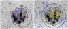 |
Fig. 1 eROSITA exposure-corrected map of G18.95-1.1 and its surrounding area. The ASCA GIS and Chandra FOVs are shown in the left panel map in black and blue. Small red circles show the location of point sources that are excluded from the spectral analysis. The brightest point source is marked with a 1, and the pulsar candidate source is marked with a P. Hα contours from the SHASSA survey (Gaustad et al. 2001), shown as blue curves, are superposed in the right panel map together with the regions we used for the spectrum analysis. The annulus we used to obtain the background spectrum is shown in black. Its inner boundary is the outer border for the SNR source region. Smaller regions that were used to extract spectra of various parts of the remnant are shown in yellow, and the brightest point source and pulsar candidate are marked in red. |
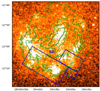 |
Fig. 2 eROSITA exposure-corrected map of G18.95-1.1 with superposed green contours of the 10.55 GHz radio emission (contours by E. Fürst) from Harrus et al. (2004). The composite SR region encompassing regions box2, C3, and C4 is shown by the blue boxes. |
Point sources excluded from the spectral analysis.
One-component CIE (APEC) spectral models for a low-temperature local χ2 minimum.
One-component NEI (PSHOCK) spectral models for a high-temperature local χ2 minimum.
One-component CIE (VAPEC) and NEI (VPSHOCK) spectral models with variable abundances.
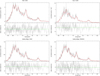 |
Fig. 3 Spectra of the whole SNR, box2, and SR regions fit with spectrum models with variable abundances of Ne, Mg, Si, and Fe (the Ni abundance was assumed equal to Fe). Upper left panel: spectrum of the whole SNR with the VAPEC model. Upper right panel: spectrum of the box2 region with the VAPEC model. Lower left panel: spectrum of the SR region with the VAPEC model. Lower right panel: spectrum of the SR region with the high-temperature VPSHOCK model. Each panel shows the spectrum data (black) and model (red) in the upper graph and the residuals in the lower graph. The model parameters for these spectra are given in Table 5. |
Two-component spectral models.
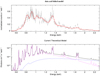 |
Fig. 4 Spectrum of the PWN region. We show spectrum data (black) and the model (red) in the upper panel and the model composition in the lower panel. The entire model is shown with the black curve, and the low-temperature apec component is shown with the magenta curve. The blue curve shows the power-law component. The model spectrum parameters are listed in Table 6. |
3 Discussion
SNR G18.95-1.1 has a complex asymmetric morphology. The bright emission regions shown in Fig. 1 are located within a ring with an inner radius of about 9′ and an outer radius of about 15′. The Hα half-shell emission excess of the same width observed in the southeast part of the remnant (SHASSA survey, Gaustad et al. 2001) coincides with the X-ray ridge (see Fig. 1).
The maximum X-ray surface brightness of the structures corresponds to the angular distance of about 12′ from the apparent center of the SNR. Therefore the outer radius of the bright ridge is within a ring 7.5 pc ≳ R ≳ 12 pc at 3 kpc distance.
The structure of the X-ray ridge in Fig. 1 has a clear large-scale asymmetry that is most prominent in the southeastern part of the SNR. The optical Hα emission in Fig. 1 (bottom panel) is more homogeneous in the field of G18.95-1.1. The X-ray ridge is not apparent in the radio images at 1.4 and 4.9 GHz presented by Furst et al. (1989), where one bright arc-like structure is associated with the PWN, while the second bright structure is located well away from the X-ray ridge. It is difficult to search for the X-ray synchrotron emission filaments produced by the ultrarelatevistic electrons accelerated at the supernova blast wave, which are more prominent in the 4–6 keV energy band, in the eROSITA observations with ~3 ks exposure, keeping in mind that it is most sensitive below 2.3 keV. The radio maps do not show any thin bright filaments that might be associated with a forward shock (Fuerst et al. 1997), however.
Core-collapse supernovae are in many cases expected to expand into a wind bubble produced by a massive progenitor star (see, e.g., Chevalier & Liang 1989; Slane et al. 2000; Dwarkadas 2005; Chevalier & Fransson 2017, and the references therein).
The lack of a clear signature of the forward shock (or outer shells) in the northern part of the G18.95-1.1 eROSITA and radio images can be understood if the asymmetric supernova ejecta is expanding in the diluted matter of the wind cavern. The broad clumpy southern X-ray ridge structure may be a result of the gas heating by the reverse shock that passed the ejecta (see, e.g., Chevalier & Fransson 2017; Vink 2017; Raymond 2018). The ejecta are clumped because of hydrodynamical instabilities. The apparent north-south asymmetry of the emitting clumps can be a result of the recoil of the ejecta in the southern direction, just in the opposite direction to the apparent proper motion of the pulsar, which produces the observed elongated bow-shock-like PWN. The asymmetry of ejecta in Cas A and some other SNRs observed in the optical, radio, and X-ray bands by Fesen (2001), Milisavljevic & Fesen (2015), Slane et al. (2015), Arias et al. (2018), and Orlando et al. (2021) was explained as due to the NS kick in the asymmetric core collapse (see, e.g., Holland-Ashford et al. 2017; Laming & Temim 2020). Recently, asymmetric X-ray structures were studied with Chandra in shocked ejecta of core-collapsed SNR G320.4-1.2/MSH 15–52, where Ne-Mg rich ejecta were found (Borkowski et al. 2020).
The ionization timescale parameter in Table 4 for the clumps of the SR derived with the PSHOCK spectral model of the temperature T ~ 0.6 keV is consistent with the characteristic age of the shocked plasma of 4000–6000 yr, which was earlier estimated by Furst et al. (1989), Harrus et al. (2004), and Tüllmann et al. (2010). The spectral model with T ~ 0.3 keV requires a minimum ionization timescale of ~1012 s cm−3, which would rather imply an older age of ≳104 yr.
The single-component spectral models presented in Table 5 clearly favor the high overabundance of Si compared to the solar composition in the SR regions. The NEI VPSHOCK model for the SR region have statistically acceptable fits for metal-rich ejecta with somewhat different temperatures of about 0.3 and 0.6 keV, respectively (and ionization timescales ≳1012 and  ), while the CIE VAPEC model allows only the low-temperature solution. The low-temperature NEI VPSHOCK fit (not shown in Table 5) requires a high value of the ionization timescale, so that the CIE VAPEC model is appropriate in this case. To study the composition of the SR and box2 regions, we fixed the abundances of C, N, O at the solar values because the available count statistics and relatively high NH values estimated for G18.95-1.1 do not allow us to obtain meaningful estimates of the C, N, O abundances. We found that a good CIE VAPEC model fit with a fixed O abundance provided Si/O and Si/Fe of ~5–8 and Si/Mg and Si/Ne of ~3–4 We recall the nearby Vela SNR (see, e.g., Miyata et al. 2001), where the situation was more favorable for studies of abundance variations, including that of the oxygen.
The X-ray image of the Vela SNR obtained with ROSAT by Aschenbach et al. (1995) discovered six extended X-ray features outside the forward shock. It was proposed that these features are fast-moving ejecta fragments formed by instabilities during the collapse of the progenitor star. Two of the fragments, dubbed shrapnel A and G, are located at the northeastern and southwestern edges of the Vela SNR, respectively. Using a single-temperature NEI model with T ~ 0.5 keV, Katsuda & Tsunemi (2006) estimated the abundances in shrapnel A to be O ~ 0.3, Ne ~ 0.9, Mg ~ 0.8, Si ~ 3, and Fe ~ 0.8 relative to their solar values. A similar Si-rich composition with relatively weak abundances of O, Ne, Mg, and Fe was derived with the two-temperature CIE and single-temperature NEI models from XMM-Newton spectra of shrapnel G García et al. (2017). Moreover, the Si-group-illuminated jets or pistons in Cas A are very prominent in X-ray, optical, and infrared emission (see, e.g., DeLaney et al. 2010; Lopez & Fesen 2018). A possible way of formation of the bright rings of Si/S-rich material was demonstrated in the modeling of asymmetric ejecta of Cas A by Orlando et al. (2016). The high ratios of Si/O ~ 5–10 derived in shrapnels A and G in the Vela SNR and in the bright southern clumps in G18.95-1.1 may be understood if the observed ejecta material came from the deep inner layers of the progenitor star.
The X-ray emitting mass in G18.95-1.1 can be estimated from the apparent angular sizes of the SR clumps given in Table 1 and the X-ray flux normalization factors derived in the single-component spectral models listed in Table 5. Assuming some simplified geometry of the clumps and given the uncertainties mentioned above, we can estimate the mass of X-ray emitting plasma as a few solar masses. Most of the emission from the SR region comes from the cores of three clumps (C1, box2, and C3). All of them have comparable values of the τu parameter of ~3 × 10¹¹ s cm−3 derived in the Table 4 and radii about 2 arcmin. Assuming the age of G18.95-1.1 to be younger than 10 000 yr and a distance of 3 kpc, we can estimate the X-ray emitting clump masses to be just above one solar mass, which is consistent with the mass estimates obtained from the spectrum normalization given in Table 5. Deep multiwavelength observations of the SNR G18.95-1.1 ridge are required to reduce the uncertainties in the spectral model and obtain more accurate mass estimation.
There are some known uncertainties (see, e.g., Greco et al. 2020) in supernova ejecta mass estimations from the plasma emission measure due to the degeneracy between the derived best-fit values of element abundances (namely a possibility of helium-rich ejecta, which is hard to constrain from X-rays). Therefore it is difficult to estimate the metal ejecta mass. Only the total X-ray emitting mass and the relative abundances of some elements can be estimated at the current level. The presence of the PWN (see Tüllmann et al. 2010) and the ejecta mass of a few M⊙ estimated above are consistent with a type Ib or IIb SN from a moderately massive progenitor star with an initial mass below 20 M⊙.
We found in the spectra of the clumps (box2, C1, and C3), the SR, and the whole SNR G18.95-1.1 marginally significant spectral features at photon energies in the range 1.2–1.3 keV. If real, these spectral features could be attributed to the emission of Fe XVII - Fe XX from the Fe L complex (Gu et al. 2019), or as an alternative explanation, the 1.2–1.3 keV residuals could be the emission of Ne X Lyβ, Lyγ, and Lyδ lines (Cumbee et al. 2016). However, more observations are needed to confirm or reject the apparent spectral excess.
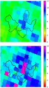 |
Fig. 5 Hydrogen column density maps in the direction to SNR G18.95-1.1 derived from the bayestar19 data cubes (Green et al. 2019) using the DUSTMAPS Python package (Green 2018) for the two distances of 2 kpc (upper panel) and of 3 kpc (bottom panel). The contours of the X-ray emission as detected by SRG eROSITA in Fig. 1 are overlaid in both panels. The color-map bars show the estimated NH values in units of 1021 cm−2. |
4 Summary
The X-ray eROSITA image of G18.95-1.1 revealed a complex asymmetric structure with a bright ridge of emission located mainly in the SE part of the remnant and a bright radially elongated structure. This structure was found in the radio imaging, and Chandra observations later confirmed that it is most likely a PWN. The apparent position and shape of the bow-shock-type PWN indicate a pulsar proper velocity of a few hundred km s−1. The asymmetric shape of the X-ray ridge may be understood as the result of a recoil of the material that is ejected after the core collapse and given the direction of apparent motion of the pulsar due to its initial kick.
The wide FOV of eROSITA and the scanning observation mode provided a fairly uniform exposure across the SNR. This allowed us to study different background models. The column density values NH ~ (7.5–10) × 1021 cm−2 derived here from the spectra of the clump regions and the whole SNR generally agree with that obtained from the ASCA data analysis by Harrus et al. (2004) and Chandra studies of the PWN region by Tüllmann et al. (2010). These NH values are greater than those that were estimated earlier in a ROSAT data analysis (Aschenbach et al. 1991; Fuerst et al. 1997) and HI radio observations by Furst et al. (1989). The high Nh values obtained in the X-ray data analysis of ASCA, Chandra, and eROSITA suggest that the distance to G18.95-1.1 is about 3 kpc, as illustrated in Fig. 5, while the issue requires further study.
The good spectral resolution of eROSITA revealed a double-peaked spectral structure just below 1 keV, where two spectral features of Fe-L and Ne lines at energies about 0.8 and 0.9 keV are clearly separated. In the eROSITA data analysis of G18.95-1.1, we have modeled the X-ray emission from the spatially resolved structures with both the collisional ionization equilibrium and nonequilibrium ionization XSPEC models. The single thermal CIE model with variable abundances provides satisfactory fits for both the dim northern region and the X-ray bright SR with a temperature about 0.3–0.4 keV. However, while the northern regions with temperatures ~0.4 keV allow for a solar composition, the bright southern regions require a strong silicon overabundance with a lower temperature ~0.3 keV. Alternatively, the southern regions can be fitted with a single-temperature NEI model with a temperature ~0.6 keV and a strong Si overabundance as well. The Si-rich clumps in G18.95-1.1 are similar to the ejecta shrapnel A and G discovered in the Vela SNR. The X-ray morphology and spectra of G18.95-1.1 detected with eROSITA can be understood in the scenario of a core-collapse supernova with Si-rich ejecta fragments that expanded into the wind of the massive progenitor star.
Acknowledgements.
This work is based on observations with eROSITA telescope onboard SRG observatory. The SRG observatory was built by Roskosmos in the interests of the Russian Academy of Sciences represented by its Space Research Institute (IKI) in the framework of the Russian Federal Space Program, with the participation of the Deutsches Zentrum für Luft- und Raumfahrt (DLR). The SRG/eROSITA X-ray telescope was built by a consortium of German Institutes led by MPE, and supported by DLR. The SRG spacecraft was designed, built, launched and is operated by the Lavochkin Association and its subcontractors. The science data are downlinked via the Deep Space Network Antennae in Bear Lakes, Ussurijsk, and Baykonur, funded by Roskosmos. The eROSITA data used in this work were processed using the eSASS software system developed by the German eROSITA consortium and proprietary data reduction and analysis software developed by the Russian eROSITA Consortium. The authors thank the anonymous referee for a careful reading of the paper and helpful comments which we used to improve the data analysis and interpretation. The authors thank R.A. Sunyaev for a helpful comment. A.M.B. and Yu.A.U. were supported by the RSF grant 21-72-20020. Some of the modeling was performed at the Joint Supercomputer Center (JSCC) RAS and at the “Tornado” subsystem of the St. Petersburg Polytechnic University supercomputing center.
References
- Acero, F., Ackermann, M., Ajello, M., et al. 2016, ApJS, 224, 8 [NASA ADS] [CrossRef] [Google Scholar]
- Arias, M., Vink, J., de Gasperin, F., et al. 2018, A&A, 612, A110 [NASA ADS] [CrossRef] [EDP Sciences] [Google Scholar]
- Arnaud, K. A. 1996, ASP Conf. Ser., 101, 17 [Google Scholar]
- Aschenbach, B., Brinkmann, W., Pfeffermann, E., Fuerst, E., & Reich, W. 1991, A&A, 246, L32 [NASA ADS] [Google Scholar]
- Aschenbach, B., Egger, R., & Trümper, J. 1995, Nature, 373, 587 [Google Scholar]
- Barnes, P. J., & Turtle, A. J. 1988, IAU Colloq., 101, 347 [NASA ADS] [Google Scholar]
- Borkowski, K. J., Lyerly, W. J., & Reynolds, S. P. 2001, ApJ, 548, 820 [Google Scholar]
- Borkowski, K. J., Miltich, W., & Reynolds, S. P. 2020, ApJ, 905, L19 [NASA ADS] [CrossRef] [Google Scholar]
- Bykov, A. M., Amato, E., Petrov, A. E., Krassilchtchikov, A. M., & Levenfish, K. P. 2017, Space Sci. Rev., 207, 235 [CrossRef] [Google Scholar]
- Chevalier, R. A., & Fransson, C. 2017, in Handbook of Supernovae, eds. A. W. Alsabti, & S. Murdin, Paul (Berlin: Springer), 875 [CrossRef] [Google Scholar]
- Chevalier, R. A., & Liang, E. P. 1989, ApJ, 344, 332 [NASA ADS] [CrossRef] [Google Scholar]
- Chevalier, R. A., & Reynolds, S. P. 2011, ApJ, 740, L26 [NASA ADS] [CrossRef] [Google Scholar]
- Cumbee, R. S., Liu, L., Lyons, D., et al. 2016, MNRAS, 458, 3554 [NASA ADS] [CrossRef] [Google Scholar]
- DeLaney, T., Rudnick, L., Stage, M. D., et al. 2010, ApJ, 725, 2038 [Google Scholar]
- Dwarkadas, V. V. 2005, ApJ, 630, 892 [NASA ADS] [CrossRef] [Google Scholar]
- Fesen, R. A. 2001, ApJS, 133, 161 [Google Scholar]
- Foight, D. R., Güver, T., Özel, F., & Slane, P. O. 2016, ApJ, 826, 66 [Google Scholar]
- Fuerst, E., Reich, W., Reich, P., Sofue, Y., & Handa, T. 1985, Nature, 314, 720 [NASA ADS] [CrossRef] [Google Scholar]
- Fuerst, E., Reich, W., & Aschenbach, B. 1997, A&A, 319, 655 [NASA ADS] [Google Scholar]
- Furst, E., Hummel, E., Reich, W., et al. 1989, A&A, 209, 361 [NASA ADS] [Google Scholar]
- Garcia, F., Suarez, A. E., Miceli, M., et al. 2017, A&A, 604, L5 [CrossRef] [EDP Sciences] [Google Scholar]
- Gaustad, J. E., McCullough, P. R., Rosing, W., & Van Buren, D. 2001, PASP, 113, 1326 [NASA ADS] [CrossRef] [Google Scholar]
- Greco, E., Vink, J., Miceli, M., et al. 2020, A&A, 638, A101 [NASA ADS] [CrossRef] [EDP Sciences] [Google Scholar]
- Green, G. 2018, J. Open Source Softw., 3, 695 [NASA ADS] [CrossRef] [Google Scholar]
- Green, G. M., Schlafly, E., Zucker, C., Speagle, J. S., & Finkbeiner, D. 2019, ApJ, 887, 93 [NASA ADS] [CrossRef] [Google Scholar]
- Gu, L., Raassen, A. J. J., Mao, J., et al. 2019, A&A, 627, A51 [NASA ADS] [CrossRef] [EDP Sciences] [Google Scholar]
- Harrus, I. M., Slane, P. O., Hughes, J. P., & Plucinsky, P. P. 2004, ApJ, 603, 152 [NASA ADS] [CrossRef] [Google Scholar]
- Holland-Ashford, T., Lopez, L. A., Auchettl, K., Temim, T., & Ramirez-Ruiz, E. 2017, ApJ, 844, 84 [Google Scholar]
- Kaastra, J. S., & Jansen, F. A. 1993, A&AS, 97, 873 [NASA ADS] [Google Scholar]
- Katsuda, S., & Tsunemi, H. 2006, ApJ, 642, 917 [Google Scholar]
- Laming, J. M., & Temim, T. 2020, ApJ, 904, 115 [NASA ADS] [CrossRef] [Google Scholar]
- Lopez, L. A., & Fesen, R. A. 2018, Space Sci. Rev., 214, 44 [NASA ADS] [CrossRef] [Google Scholar]
- Mewe, R., Gronenschild, E. H. B. M., & van den Oord, G. H. J. 1985, A&AS, 62, 197 [NASA ADS] [Google Scholar]
- Milisavljevic, D., & Fesen, R. A. 2015, Science, 347, 526 [NASA ADS] [CrossRef] [Google Scholar]
- Miyata, E., Tsunemi, H., Aschenbach, B., & Mori, K. 2001, ApJ, 559, L45 [NASA ADS] [CrossRef] [Google Scholar]
- NASA High Energy Astrophysics Science Archive Research Center -HEASARC-2014, HEAsoft: Unified Release of FTOOLS and XANADU [Google Scholar]
- Odegard, N. 1986, AJ, 92, 1372 [NASA ADS] [CrossRef] [Google Scholar]
- Orlando, S., Miceli, M., Pumo, M. L., & Bocchino, F. 2016, ApJ, 822, 22 [Google Scholar]
- Orlando, S., Wongwathanarat, A., Janka, H. T., et al. 2021, A&A, 645, A66 [EDP Sciences] [Google Scholar]
- Patnaik, A. R., Velusamy, T., & Venugopal, V. R. 1988, Nature, 332, 136 [NASA ADS] [CrossRef] [Google Scholar]
- Predehl, P., Andritschke, R., Arefiev, V., et al. 2021, A&A, 647, A1 [EDP Sciences] [Google Scholar]
- Raymond, J. C. 2018, Space Sci. Rev., 214, 28 [NASA ADS] [CrossRef] [Google Scholar]
- Reich, W. 2002, in Neutron Stars, Pulsars, and Supernova Remnants, eds. W. Becker, H. Lesch, & J. Trümper (USA: NASA), 1 [Google Scholar]
- Reich, W., Fuerst, E., Haslam, C. G. T., Steffen, P., & Reif, K. 1984, A&AS, 58, 197 [NASA ADS] [Google Scholar]
- Slane, P., Chen, Y., Schulz, N. S., et al. 2000, ApJ, 533, L29 [NASA ADS] [CrossRef] [Google Scholar]
- Slane, P., Bykov, A., Ellison, D. C., Dubner, G., & Castro, D. 2015, Space Sci. Rev., 188, 187 [NASA ADS] [CrossRef] [Google Scholar]
- Stupar, M., & Parker, Q. A. 2011, MNRAS, 414, 2282 [Google Scholar]
- Sun, X. H., Reich, P., Reich, W., et al. 2011, A&A, 536, A83 [EDP Sciences] [Google Scholar]
- Sunyaev, R., Arefiev, V., Babyshkin, V., et al. 2021, A&A, 656, A132 [NASA ADS] [CrossRef] [EDP Sciences] [Google Scholar]
- Tüllmann, R., Plucinsky, P. P., Gaetz, T. J., et al. 2010, ApJ, 720, 848 [CrossRef] [Google Scholar]
- Vink, J. 2017, in Handbook of Supernovae, eds. A. W. Alsabti, & S. Murdin, (Berlin: Springer), 2063 [CrossRef] [Google Scholar]
- Wilms, J., Allen, A., & McCray, R. 2000, ApJ, 542, 914 [Google Scholar]
Here and below, the element abundances are measured relative to solar abundances.
All Tables
One-component NEI (PSHOCK) spectral models for a high-temperature local χ2 minimum.
One-component CIE (VAPEC) and NEI (VPSHOCK) spectral models with variable abundances.
All Figures
|
Fig. 1 eROSITA exposure-corrected map of G18.95-1.1 and its surrounding area. The ASCA GIS and Chandra FOVs are shown in the left panel map in black and blue. Small red circles show the location of point sources that are excluded from the spectral analysis. The brightest point source is marked with a 1, and the pulsar candidate source is marked with a P. Hα contours from the SHASSA survey (Gaustad et al. 2001), shown as blue curves, are superposed in the right panel map together with the regions we used for the spectrum analysis. The annulus we used to obtain the background spectrum is shown in black. Its inner boundary is the outer border for the SNR source region. Smaller regions that were used to extract spectra of various parts of the remnant are shown in yellow, and the brightest point source and pulsar candidate are marked in red. |
| In the text | |
|
Fig. 2 eROSITA exposure-corrected map of G18.95-1.1 with superposed green contours of the 10.55 GHz radio emission (contours by E. Fürst) from Harrus et al. (2004). The composite SR region encompassing regions box2, C3, and C4 is shown by the blue boxes. |
| In the text | |
|
Fig. 3 Spectra of the whole SNR, box2, and SR regions fit with spectrum models with variable abundances of Ne, Mg, Si, and Fe (the Ni abundance was assumed equal to Fe). Upper left panel: spectrum of the whole SNR with the VAPEC model. Upper right panel: spectrum of the box2 region with the VAPEC model. Lower left panel: spectrum of the SR region with the VAPEC model. Lower right panel: spectrum of the SR region with the high-temperature VPSHOCK model. Each panel shows the spectrum data (black) and model (red) in the upper graph and the residuals in the lower graph. The model parameters for these spectra are given in Table 5. |
| In the text | |
|
Fig. 4 Spectrum of the PWN region. We show spectrum data (black) and the model (red) in the upper panel and the model composition in the lower panel. The entire model is shown with the black curve, and the low-temperature apec component is shown with the magenta curve. The blue curve shows the power-law component. The model spectrum parameters are listed in Table 6. |
| In the text | |
|
Fig. 5 Hydrogen column density maps in the direction to SNR G18.95-1.1 derived from the bayestar19 data cubes (Green et al. 2019) using the DUSTMAPS Python package (Green 2018) for the two distances of 2 kpc (upper panel) and of 3 kpc (bottom panel). The contours of the X-ray emission as detected by SRG eROSITA in Fig. 1 are overlaid in both panels. The color-map bars show the estimated NH values in units of 1021 cm−2. |
| In the text | |
Current usage metrics show cumulative count of Article Views (full-text article views including HTML views, PDF and ePub downloads, according to the available data) and Abstracts Views on Vision4Press platform.
Data correspond to usage on the plateform after 2015. The current usage metrics is available 48-96 hours after online publication and is updated daily on week days.
Initial download of the metrics may take a while.