| Issue |
A&A
Volume 660, April 2022
|
|
|---|---|---|
| Article Number | A55 | |
| Number of page(s) | 7 | |
| Section | The Sun and the Heliosphere | |
| DOI | https://doi.org/10.1051/0004-6361/202143021 | |
| Published online | 12 April 2022 | |
Magnetic field evolution around a fast-moving pore emerging from the quiet Sun⋆
1
Key Laboratory of Dark Matter and Space Astronomy, Purple Mountain Observatory, Chinese Academy of Sciences, No. 8 Yuanhua Road, Qixia District, Nanjing 210034, PR China
e-mail: This email address is being protected from spambots. You need JavaScript enabled to view it.
2
Yunnan Observatories, Chinese Academy of Sciences, 396 Yangfangwang, Guandu District, Kunming 650216, PR China
Received:
31
December
2021
Accepted:
10
February
2022
Abstract
Context. Solar pores are intense concentrations of magnetic fields on the solar surface and plasma flows have always played a key role in spurring the evolution of the pores.
Aims. In this study, we present the evolution of the magnetic field and plasma velocity around a fast-moving pore. The target pore expands into the quiet Sun area with a sufficiently fast speed after its emergence, while the background magnetic fields around the pore are simple. These characteristics provide us with an excellent opportunity to study the interaction between plasma motions and ambient magnetic fields.
Methods. We analyzed the Helioseismic and Magnetic Imager (HMI) vector magnetograms with a pixel size of 0.5″ and a temporal cadence of 12 min across a duration of 11 h. We also adopted he HMI dopplergrams present the line-of-sight velocities. The horizontal flow fields were obtained using the Differential Affine Velocity Estimator for Vector Magnetograms method.
Results. Pure horizontal magnetic fields are generated in the moving frontwards when the pore is subject to fast movement. The generated magnetic fields occur outside the emerging site and thus can be ruled out as the emerging flux from the interior. Instead, they are highly correlated with the broader downflows and expanding horizontal plasma motions in front of the pore. A magnetic gap can be observed between the magnetic fields inside and outside the pore. The temporal evolution of the generated magnetic fields is related to the speed of the pore, which is also distinguished from the original fields within the pore.
Conclusions. The observations suggest that the plasma flows driven by the fast proper motion of the pore compress and stretch the local magnetic field to a horizontal non-radial direction, ultimately leading to the magnetic field amplification in the front part of the moving pore.
Key words: Sun: magnetic fields / Sun: photosphere / sunspots
Movie associated to Fig. 1 is available at https://www.aanda.org
Present address: Purple Mountain Observatory, Chinese Academy of Sciences, No. 8 Yuanhua Road, Qixia District, Nanjing 210034, PR China.
© ESO 2022
1. Introduction
Pores are a common feature in the solar photosphere, characterized by sunspots without penumbrae (Bray & Loughhead 1964; Leka & Skumanich 1998; Sobotka 2003; Solanki 2003). They are intense concentrations of the nearly vertical magnetic field, with a field strength of several kG and an intermediate size of a few Mm (Keppens & Martinez Pillet 1996). Varied from the small-scale magnetic elements such as the photospheric bright faculae and network (Ortiz et al. 2002), the magnetic fields of pores are strong enough to inhibit the convective energy transport, thus creating darker compact regions on the solar surface. Meanwhile, the absence of penumbrae indicates that the pores have rather simple and unified magnetic structures compared to large structures such as mature sunspots (Simon & Weiss 1970). Accordingly, pores have been a suitable object for studying magnetohydrodynamics on the Sun through an investigation of their magnetic properties and dynamic evolutions (Cameron et al. 2007; Morton et al. 2011).
The temporal evolutions of fine structures and magnetic fields around pores have been investigated in recent decades (Leka & Skumanich 1998; Sobotka et al. 1999; Hirzberger 2003; García-Rivas et al. 2021), including the emergence and formation of pores (Zwaan 1992; Wang & Zirin 1992; Ermolli et al. 2017), development into mature sunspots (Schlichenmaier et al. 2010; Murabito et al. 2018), and the decay process (Murabito et al. 2021; Xue et al. 2021). Over the course of the entire process. Plasma flows play a key role in promoting the evolution of the pores. Observations show that horizontal flow convergence is co-spatial with downflows in the areas of pores, suggesting that pores are formed through a convective collapse mechanism (Zwaan 1985; Keil et al. 1999; Sobotka 2003; Hirzberger 2003). Keil et al. (1999) proposed that the perturbation from exploding granules could initiate the rapid formation of a penumbra around the pore. Murabito et al. (2016) found that the annular zone around the pore is characterized by downflows before the penumbra is formed, suggesting that the effect of the magnetic field sinking down to the photosphere could lead to the penumbra formation. The decay of the pore is considered to be the result of turbulent erosion, through a process that involves the magnetic field gradually leaking out and dispersing into the adjacent intergranular lanes (Petrovay & Moreno-Insertis 1997; Cameron et al. 2007). On the other hand, the existence of a magnetic field could, in turn, affect the plasma motions. Roudier et al. (2002) asserted that the plasma velocities inside the pore are smaller by a factor of two than those outside the pore. Hirzberger (2003) reported that the plasma motions within the pore are almost completely inhibited by the magnetic field and that they show obvious asymmetry around. Sobotka et al. (2012) also found that both line-of-sight and horizontal plasma motions are suppressed by the magnetic field inside the pore.
Recent observations have revealed that the interaction between plasma motions and magnetic field can give rise to magnetic field amplification through magnetic induction. Shimizu et al. (2008) found that the magnetic elements can be amplified by local mass downflows on the solar surface. Narayan (2011) presents eight cases of magnetic field intensification involving strong transient downflows, and all cases are associated with the formation of a bright point in the continuum. Ermolli et al. (2017) reported that some amplification and structuring effects by surface plasma motions occur in the emerged field during the formation of a pore. Xu et al. (2020) reported that the expanding flows in front of a pore can lead to the formation of non-radial penumbra structures. More examples can also be found in the sunspots with stronger and more complex magnetic fields (Okamoto & Sakurai 2018; Castellanos Durán et al. 2020).
In this article, we investigate the magnetic field evolution of a fast-moving pore emerging from the quiet Sun. The rapid passage of the pore across the solar surface provides us prime opportunity to shed light on the interaction between plasma flow and magnetic field. The whole course of the motion was aptly recorded by the observations from HMI vector magnetograms. We performed the magnetic field analysis and tracked the horizontal and line-of-sight plasma flow. We present the correlation between the magnetic fields and plasma velocities, with the goal of demonstrating that the magnetic field in front of the pore is amplified by the proper motion of the pore.
2. Observations and data processing
The observations used in this study were provided by the Helioseismic and Magnetic Imager (HMI; Schou et al. 2012) on board the Solar Dynamics Observatory (SDO; Pesnell et al. 2012). HMI takes full-disk continuum images and line-of-sight magnetograms with a pixel size of 0.5″ and 45 s cadence. It also provides the vector magnetic field data of Space weather HMI Active Region Patches (SHARPs; Bobra et al. 2014), with a pixel size of 0.5″ and 12 min cadence. The measurement accuracy is ∼10 G/∼100 G for the vertical-horizontal component. The remaining 180° azimuth ambiguity was resolved by using the Minimum Energy code (Metcalf 1994; Leka et al. 2009). The vector magnetograms have been remapped using a Lambert cylindrical equal area projection, providing the horizontal and vertical magnetic field (Bx, y, z). Then the vector magnetograms are transformed into a standard heliographic spherical coordinates to match the continuum images. The line-of-sight velocity data are provided by the HMI dopplergrams, with a pixel size of 0.5″ and 45 s cadence. We calibrated the dopplergrams by assuming that the convective blueshift of the quiet Sun has an average velocity value of about −100 ms−1. The photospheric horizontal velocity data are derived by applying the Differential Affine Velocity Estimator for Vector Magnetograms algorithm (DAVE4VM; Schuck 2008) on the HMI vector magnetograms. The window size is set to 10 pixels, corresponding to the magnetic features with a spatial scale of 5″. All of the above data are rotated to a reference time at 00:00 UT on 2012 February 6.
3. Results
3.1. Overview of the rapidly moving pore in HARP 1367
The event that is the focus of this article occurred in a newly emerging flux region near the center of the solar disk (N10W18) on 2012 February 6. The emerging flux is relatively small and therefore it was not recorded by the National Oceanic and Atmospheric Administration/Space Weather Prediction Center (NOAA/SWPC) as an active region. However, HMI did name it HARP 1367 and provided continuum images and magnetic field measurements during its disk passage. As shown in Fig. 1 and the accompanying online animation, a simple bipolar emerges from the quiet Sun and then the opposite magnetic polarities expand away from the emergence site immediately. The negative preceding polarities have stronger magnetic fields and move faster than the following ones, showing a small pore moving rapidly to the southwest after it appears on the surface, as highlighted by the red arrow in Fig. 1b. Intriguingly, line-of-sight magnetic fields can be detected in front of the pore (Fig. 1c and online animation). The strength of these magnetic fields is greater than 100 G, which is well above the measurement accuracy. These line-of-sight magnetic fields are unstable and appear only when the pore is under rapid proper motion; in particular, they move synchronously with the pore. Considering the location of these magnetic fields is on the far side of the emerging flux area, we infer that the magnetic flux in this region probably does not come from the emergence but, rather, it is an accompanying phenomenon related to the movement of the pore.
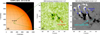 |
Fig. 1. Overview of the rapidly moving pore in HARP 1367 observed by SDO/HMI. Panel a: HMI continuum image shows the northwest quadrant of the solar disk on 2012 February 6. The target region is located at N10W18 as indicated by the green box. Panels b,c: close-up views of the HMI continuum image and line-of-sight magnetogram during the flux emergence. The red arrow in panel b indicates the direction of the pore movement. The blue arrows in panel c mark the emerging flux elements. The cyan arrow in panel c points to the appearance of the weak magnetic fields in front of the pore. An animation is available online to show the dynamic details. The animated images run from 2012 February 5 20:00 UT to 2012 February 6 07:56 UT. |
3.2. Magnetic field analysis
Figure 2 shows snapshots of the continuum intensity, the vertical magnetic field strength, the total magnetic field strength, and the magnetic field inclination around the moving pore before, during, and after the fast movement. In general, strong magnetic fields are concentrated in the region where the pores are located and most of them are composed of vertical magnetic fields. Taking the target sunspot as an example, at the beginning (02-05/22:00 UT), the average total magnetic field in the pore region (white circle) is 730 G, of which the vertical field is 620 G. These two values are 1000/890 G during the fast movement phase (02-06/01:24 UT), and 1200/1080 G after (02-06/07:12 UT). According to the maps of magnetic field inclination, the average inclination angle in the pore region at three times is 57, 64, and 66°, respectively, indicating that the magnetic field of the pore is primarily vertical during its entire evolution. However, when the pore is subject top fast movement, strong magnetic fields suddenly appear right in front of the pore, but the vertical component is quite weak instead as indicated by the cyan arrows in Figs. 2b2 and c2. The average total-vertical magnetic field in the dotted rectangle area is 330/40 G, showing a nearly horizontal pattern. As is also seen from the inclination map (Fig. 2d2), a very flat zone is created in front of the moving pore. The average inclination angle in the dotted rectangle area is 8°, which is very distinct from the pore and surrounding quiet Sun; whereas after the fast movement, the magnetic fields in front of the pore return to normal as the surrounding area.
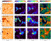 |
Fig. 2. Maps of continuum intensity (panels a1–a3), vertical magnetic field strength (panels b1–b3), total magnetic field strength (panels c1–c3), and magnetic field inclination (panels d1–d3) at three selected times before, during, and after the rapid movement of the pore (from left to right). The inclination angle is defined as with respect to the photospheric surface, i.e., 0° is horizontal, while that of 90° is vertical. The white circle in each panel marks the position of the moving pore. The cyan arrow in panels b2, c2, and d2 points to the dotted rectangle area in front of the moving pore. The field of view is 30″ × 30″ centered at the target pore. |
The above observations suggest that pure horizontal magnetic fields are generated when the pore is subject to fast movement. Figures 3a–c present the HMI vector magnetograms in HARP 1367 at three times corresponding to Fig. 2. Indeed, a large number of horizontal magnetic fields appear on the surface following the flux emergence and fast movement of the pore (Fig. 3b). However, differences in morphology can be found between the magnetic fields in the emerging flux region and front of the pore. Within the emerging flux region, the horizontal magnetic fields are directed from the positive polarities to the negative polarities, showing a configuration of the Ω-loop emergence (Zwaan 1992; Lites et al. 1998). When in front of the pore, the horizontal magnetic fields wrap in a semicircular direction in a way that is consistent with the localized amplification of horizontal fields, as previously reported by Xu et al. (2020). The region of the amplified horizontal magnetic field coincides with the appearance of the line-of-sight magnetic field mentioned before. But the strength of the horizontal fields is about 400 G, which is much stronger than the line-of-sight magnetic fields. Considering that the vertical component is relatively weak in this location, we speculate that the line-of-sight magnetic field might be a projection of the horizontal magnetic fields. In this assumption, line-of-sight magnetic fields with negative polarity need to be projected from a horizontal magnetic field pointing away from the disk center. According to the HMI vector magnetogram with its 180° azimuth ambiguity resolved, the horizontal fields are mostly in the northwest direction, which precisely confirms our assumption. Moreover, at the position around 10° N, 18° W, the projection angle of the horizontal direction to the line-of-sight direction is about 20°, allowing the horizontal magnetic fields with a strength of ∼400 G to project to the line-of-sight magnetic fields with a strength of ∼100 G.
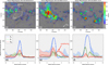 |
Fig. 3. HMI vector magnetograms showing the evolution of HARP 1367 at three selected times corresponding to Fig. 2 shown in panels a–c. The background greyscale image shows the vertical field (Bz), and the overplotted arrows represent the horizontal fields (Bx, y) with color indicating the field strength. The vertical orange line in each panel marks the X position of the moving pore. Panels d–f: magnetic field diagnosis for the local area of moving pore. The horizontal field in the rectangular coordinate (Bx, y) has been transformed into a polar coordinate (Br, θ) with the center of the pore as the origin. The region of interest has been divided into two parts: the area moving frontwards and that moving behind, as illustrated by the two white fan-shaped areas in panela. Azimuthally averaged components of the magnetic field vector (Br, θ, z) are calculated as a function of the radial distance r from the pore center as shown by the colored curves in three panels. The positive and negative directions of the x-axis represents the radial distance in front of and behind the moving pore, respectively. |
To better figure out the magnetic configuration around the moving pore, we transformed the horizontal magnetic fields (Bx, y) to a polar coordinate (Br, θ) with the center of the pore as the origin, and then divided the region of interest into two parts: one moving in front and the other behind, as shown by two fan-shaped areas in panel a. Figures 3d–f presents the azimuthally averaged components of the magnetic field (Br, θ, z) at three selected times corresponding to the upper panels. The most remarkable feature is that Bθ is significantly amplified when the pore is under rapid proper motion during the flux emergence. The field amplification shows an asymmetry that only occurs at the moving in the front of the pore, as highlighted by the red arrow in Fig. 3e. In particular, there is an obvious gap between the amplified Bθ and the original Bθ at the edge of the pore around 1″, showing that the magnetic field amplification mainly occurs at the area outside the pore. It also can be noted that the vertical component (Bz) at the moving frontwards is fairly weak during the flux emergence. In Fig. 3e, the mean strength of Bz between 2″ and 5″ is 40 G, which is much less than Br of 100 G and Bθ of 350 G. Hence, the magnetic field shows a nearly horizontal, semicircular configuration at the local region ahead of the pore. Such a distinctive pattern further confirms our conjecture that the horizontal fields are locally amplified rather than emerging from the solar interior.
3.3. Photospheric horizontal and line-of-sight velocity
Magnetic field amplification is considered to be due to the interaction of plasma flow with the ambient magnetic field according to the MHD induction equation. Therefore, the photospheric horizontal and line-of-sight motions around the fast-moving pore are further investigated. Figures 4a–c show the horizontal proper motions at three selected times corresponding to the vector magnetograms above presented. Clearly, significant horizontal flows are created following the fast movement of the pore (Fig. 4b). These flows mainly concentrate in front of the pore and expand outwards along a radial direction. Most velocity values are greater than 500 ms−1, with a maximum of about 1500 ms−1. The velocity decreases with the increase in the distance from the pore, thus resulting in a shear action in front of the pore.
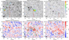 |
Fig. 4. Photospheric horizontal and line-of-sight velocity maps at three selected times corresponding to Fig. 2. Panels a–c: the background greyscale image shows the continuum image, and the overplotted arrows represent the horizontal flow fields (Vx, y) derived by using the DAVE4VM method, with color indicating the velocity. Panels d–f: HMI dopplergrams (Vlos) with the blue and red patches indicate upflows and downflows, respectively. The black contours represent the pore boundaries with intensity level I/IqS = 0.9. The green contours in panel e outlines the region with horizontal velocity greater than 500 ms−1. The vertical red line in each panel marks the X position of the moving pore. |
Figures 4d–f presents the maps of line-of-sight velocity. The result shows that downflows (corresponding to positive values) continuously appear in the fast-moving pore and its periphery. The downflows start with about 300 ms−1 before the fast movement of the pore. Then they become stronger and expand to a wider area when the pore is under the fast movement, with a mean velocity of 540 ms−1 and a maximum of about 1000 ms−1. As the pore slows down, the downflows decrease to 340 ms−1 eventually. Particularly, when the contours of horizontal flows with a level of 500 ms−1 are overplotted in Fig. 4e, it is found that the significant horizontal flows mostly coincides with the broader downflows around the pore.
Both the horizontal and line-of-sight velocity maps indicate that obvious plasma flows occur around the pore when it expands rapidly into the quiet Sun area. It is worth noting that the plasma flows also show an asymmetry that mainly appears in front of the pore, coinciding with the location where the horizontal magnetic fields are amplified, as previously observed in Fig. 3b. Therefore, the strong spatial correlation implies that the plasma motions could compress and stretch the magnetic field, leading to the amplification of the horizontal magnetic field in the photosphere.
3.4. Time evolutions
The displacement of the target pore is obtained by tracing its flux centroid from 20:00 UT of 2012 February 5 to 07:00 UT of 2012 February 6. As shown in Fig. 5a, the proper motion of the pore can be roughly divided into three phases. Initially, it presents a slow-motion with an average velocity of 280 ms−1 in Phase I. Then, due to a sudden emergence of magnetic flux, the pore is accelerated to a rapid-motion state with an average velocity of 930 ms−1 in Phase II. With the increase in distance, the pore gradually decelerates and finally returns to a slow-motion state with an average velocity of 350 ms−1 in Phase III. By using the center coordinates of the pore, a moving local frame can be established to study the evolution of the local magnetic field associated with the proper motion of the pore.
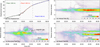 |
Fig. 5. Time evolutions of the displacement of the pore and the local magnetic field. Panel a: time profile of the displacement of the pore from 20:00 UT of 2012 February 5 to 07:00 UT of 2012 February 6. The vertical dashed line marks two times at 23:45 UT of 2012 February 5 and 02:52 UT of 2012 February 6, which divide the movement of the pore into three phases. The dashed green, red, and blue lines are the linear fits to the displacement of the pore in three phases, respectively. The mean velocity of each phase is calculated as shown by the labels. Panels b–d: time slices of the azimuthally averaged vertical field (Bz), azimuthal field (Bθ), and radial field (Br) in the local frame. The positive and negative directions of the y-axis represents the radial distance in front of and behind the moving pore, respectively. The black arrow in panel c points to the magnetic gap between the between the amplified Bθ outside and the original Bθ within the pore. The black dotted contour overplotted in each panel refers to the boundary of the amplified azimuthal field, with a strength level of 200 G. |
Figures 5b–d presents the time slices of the azimuthally averaged magnetic field (Bz, Bθ, and Br) in the local frame. It is quite obvious that Bθ undergoes a different evolution from Bz and Br. Most of the increasing Bθ occurs in Phase II and shows obvious regional asymmetry, as shown in Fig. 5c. A clear gap can also be found in the time slice of Bθ (pointed by the black arrow), confirming again that the magnetic fields at the front and within the pore belong to different systems. However, Bz and Br have no response in the region where Bθ is amplified, as shown by the dotted contour overplotted in Figs. 5b and d. The increase in these two components, Bz and Br, is concentrated in the pore region and mainly occurs in Phase III. On the contrary, the amplified Bθ decays significantly when the pore decelerates in Phase III.
Consequently, it can be inferred from the observations the manner in which each component of the magnetic field has evolved during the moving period of the pore. We can see that Bθ is amplified by the fast proper motion of the pore. It is an ephemeral phenomenon related to the speed of the pore and shows obvious spatial asymmetry in front of and behind the pore; whereas Bz and Br present a conventional evolution of a pore. The increase in their strength is due to the convergence of magnetic flux in the deceleration phase. It is quite stable and spatially symmetrical. Especially, Br separates on either side in Phase III, suggesting that the increase in Br is due to the bending of the magnetic field near the outer boundary when the magnetic flux of the pore grows sufficiently (Simon & Weiss 1970; Leka & Skumanich 1998; Rezaei et al. 2012).
4. Discussion and conclusions
In this article, we investigate the magnetic field evolution and velocity properties around a fast-moving pore. Motion-generated magnetic fields can be observed in front of the pore when it expands into the quiet Sun area. The generated magnetic fields occur outside the emerging site and thus can be ruled out as the emerging flux from the interior. Instead, they are highly correlated with the plasma flows in front of the pore. The observations suggest that the interaction between plasma flows and ambient magnetic fields could account for the localized amplification of the magnetic fields around the fast-moving pore.
In front of the pore, the non-radial component of the horizontal magnetic field is significantly amplified, but the radial and vertical components have no significant enhancement. We thus speculate that the broader downflows and the expanding horizontal flows could compress and stretch the local magnetic field lines to a horizontal non-radial direction, ultimately leading to magnetic field amplification around the moving pore. This feature is in line with previous observations and simulations. For example, Okamoto & Sakurai (2018) report that the super-strong horizontal field (6190 G) in the sunspot was generated as a result of compression by the horizontal flow. Castellanos Durán et al. (2020) detect strong horizontal fields in the sunspot light bridge associated with significant downflows. Hotta & Toriumi (2020) simulated the amplification of horizontal fields in the delta-spot light bridge caused by the rotational motion from two spots. However, the above studies take place in the mutual motion between strong magnetic fields. In this event, the magnetic fields in front of the pore are originally very weak. The amplifying process from scratch strongly suggests that magnetic induction is the main mechanism for generating magnetic fields.
Moreover, a clear magnetic gap was found between the amplified magnetic field and the original magnetic field of the pore, indicating that the field amplification mainly occurs outside the pore. The pore fields might act as a magnetic barrier as suggested by Castellanos Durán et al. (2020). Inside the pore, the plasma motion is dominated by the magnetic pressure so that the plasma moves along the magnetic field line, which cannot lead to the field amplification. While outside the pore, the dominance of plasma pressure allows the local magnetic fields to be dragged with the plasma flow to result in the field amplification. Such a scenario is similar to the view of the penumbra formation based on the plasma beta analysis (Bourdin 2017). The author suggests that the falling plasma in a regime where plasma β > 1 might be responsible for the penumbra formation outside the umbra, through dragging the magnetic field down to the photosphere.
Although the horizontal magnetic fields in front of the pore are amplified, no penumbra-like structures form in front of the pore during its passage. The total magnetic flux of the pore is on the order of 7.6 × 10¹⁹ Mx, which is less than the necessary magnetic flux for the formation of a penumbra between 1−7 × 10²⁰ Mx as concluded by previous theories and observations (Rucklidge et al. 1995; Leka & Skumanich 1998; Rezaei et al. 2012). The vertical strength near the pore boundary is on the order of 100 G, which is also less the critical value of the vertical magnetic field ∼1.8 kG required to establish a stable umbra-penumbra boundary (Jurčák et al. 2015, 2018). In this event, the amplified magnetic fields alone are not strong enough to suppress the convective heat transportation. Therefore, we can only see a pore rapidly moving across the solar surface in the photospheric continuum images. Magnetic field amplification might be universal on the solar surface, however, most magnetic field amplifications are not easily detectable because the near-surface turbulent flows are on a small scale and cannot maintain strength and stability for a relatively long time. It is hoped that higher resolution and precision magnetic measurements, such as the Daniel K. Inouye Solar Telescope (DKIST; Rimmele et al. 2020; Rast et al. 2021), will help us observe more details of magnetic field amplification on the solar surface in the future study.
Movie
Movie 1 associated with Fig. 1 (fig1anim) Access Supplementary Material
Acknowledgments
The authors would like to express their gratitude to the SDO/HMI team for providing the data. Z.X. is grateful for the hospitality of Yunnan Observatories during a visit in September 2021. This work is supported by the B-type Strategic Priority Program No. XDB41000000 funded by the Chinese Academy of Sciences, the National Key R & D Program of China (2019YFA0405000), the Project funded by China Postdoctoral Science Foundation 2020M671639, the Natural Science Foundation of China under grants 11873027, 11633008, 12073077, U2031140, 11790302, 12073072, 11873088, 12173084,12173092 and 11933009, the Scientific Research Project of “333 Projec” of Jiangsu: BRA2019310, the CAS “Light of West China” Program, and the Open Research Program of the Key Laboratory of Solar Activity of Chinese Academy of Sciences (KLSA202005).
References
- Bobra, M. G., Sun, X., Hoeksema, J. T., et al. 2014, Sol. Phys., 289, 3549 [Google Scholar]
- Bourdin, P. A. 2017, ApJ, 850, L29 [NASA ADS] [CrossRef] [Google Scholar]
- Bray, R. J., & Loughhead, R. E. 1964, Sunspots (London: Chapman and Hall) [Google Scholar]
- Cameron, R., Schüssler, M., Vögler, A., & Zakharov, V. 2007, A&A, 474, 261 [NASA ADS] [CrossRef] [EDP Sciences] [Google Scholar]
- Castellanos Durán, J. S., Lagg, A., Solanki, S. K., & van Noort, M. 2020, ApJ, 895, 129 [Google Scholar]
- Ermolli, I., Cristaldi, A., Giorgi, F., et al. 2017, A&A, 600, A102 [NASA ADS] [CrossRef] [EDP Sciences] [Google Scholar]
- García-Rivas, M., Jurčák, J., & Bello González, N. 2021, A&A, 649, A129 [NASA ADS] [CrossRef] [EDP Sciences] [Google Scholar]
- Hirzberger, J. 2003, A&A, 405, 331 [NASA ADS] [CrossRef] [EDP Sciences] [Google Scholar]
- Hotta, H., & Toriumi, S. 2020, MNRAS, 498, 2925 [NASA ADS] [CrossRef] [Google Scholar]
- Jurčák, J., Bello González, N., Schlichenmaier, R., & Rezaei, R. 2015, A&A, 580, L1 [NASA ADS] [CrossRef] [EDP Sciences] [Google Scholar]
- Jurčák, J., Rezaei, R., González, N. B., Schlichenmaier, R., & Vomlel, J. 2018, A&A, 611, L4 [NASA ADS] [CrossRef] [EDP Sciences] [Google Scholar]
- Keil, S. L., Balasubramaniam, K. S., Smaldone, L. A., & Reger, B. 1999, ApJ, 510, 422 [NASA ADS] [CrossRef] [Google Scholar]
- Keppens, R., & Martinez Pillet, V. 1996, A&A, 316, 229 [NASA ADS] [Google Scholar]
- Leka, K. D., & Skumanich, A. 1998, ApJ, 507, 454 [NASA ADS] [CrossRef] [Google Scholar]
- Leka, K. D., Barnes, G., Crouch, A. D., et al. 2009, Sol. Phys., 260, 83 [Google Scholar]
- Lites, B. W., Skumanich, A., & Martinez Pillet, V. 1998, A&A, 333, 1053 [NASA ADS] [Google Scholar]
- Metcalf, T. R. 1994, Sol. Phys., 155, 235 [Google Scholar]
- Morton, R. J., Erdélyi, R., Jess, D. B., & Mathioudakis, M. 2011, ApJ, 729, L18 [Google Scholar]
- Murabito, M., Romano, P., Guglielmino, S. L., Zuccarello, F., & Solanki, S. K. 2016, ApJ, 825, 75 [NASA ADS] [CrossRef] [Google Scholar]
- Murabito, M., Zuccarello, F., Guglielmino, S. L., & Romano, P. 2018, ApJ, 855, 58 [NASA ADS] [CrossRef] [Google Scholar]
- Murabito, M., Guglielmino, S. L., Ermolli, I., et al. 2021, A&A, 653, A93 [NASA ADS] [CrossRef] [EDP Sciences] [Google Scholar]
- Narayan, G. 2011, A&A, 529, A79 [EDP Sciences] [Google Scholar]
- Okamoto, T. J., & Sakurai, T. 2018, ApJ, 852, L16 [Google Scholar]
- Ortiz, A., Solanki, S. K., Domingo, V., Fligge, M., & Sanahuja, B. 2002, A&A, 388, 1036 [NASA ADS] [CrossRef] [EDP Sciences] [Google Scholar]
- Pesnell, W. D., Thompson, B. J., & Chamberlin, P. C. 2012, Sol. Phys., 275, 3 [Google Scholar]
- Petrovay, K., & Moreno-Insertis, F. 1997, ApJ, 485, 398 [Google Scholar]
- Rast, M. P., Bello González, N., Bellot Rubio, L., et al. 2021, Sol. Phys., 296, 70 [NASA ADS] [CrossRef] [Google Scholar]
- Rezaei, R., Bello González, N., & Schlichenmaier, R. 2012, A&A, 537, A19 [NASA ADS] [CrossRef] [EDP Sciences] [Google Scholar]
- Rimmele, T. R., Warner, M., Keil, S. L., et al. 2020, Sol. Phys., 295, 172 [Google Scholar]
- Roudier, T., Bonet, J. A., & Sobotka, M. 2002, A&A, 395, 249 [NASA ADS] [CrossRef] [EDP Sciences] [Google Scholar]
- Rucklidge, A. M., Schmidt, H. U., & Weiss, N. O. 1995, MNRAS, 273, 491 [NASA ADS] [CrossRef] [Google Scholar]
- Schlichenmaier, R., Rezaei, R., Bello González, N., & Waldmann, T. A. 2010, A&A, 512, L1 [NASA ADS] [CrossRef] [EDP Sciences] [Google Scholar]
- Schou, J., Scherrer, P. H., Bush, R. I., et al. 2012, Sol. Phys., 275, 229 [Google Scholar]
- Schuck, P. W. 2008, ApJ, 683, 1134 [NASA ADS] [CrossRef] [Google Scholar]
- Shimizu, T., Lites, B. W., Katsukawa, Y., et al. 2008, ApJ, 680, 1467 [NASA ADS] [CrossRef] [Google Scholar]
- Simon, G. W., & Weiss, N. O. 1970, Sol. Phys., 13, 85 [Google Scholar]
- Sobotka, M. 2003, Astron. Nachr., 324, 369 [Google Scholar]
- Sobotka, M., Vázquez, M., Bonet, J. A., Hanslmeier, A., & Hirzberger, J. 1999, ApJ, 511, 436 [Google Scholar]
- Sobotka, M., Del Moro, D., Jurčák, J., & Berrilli, F. 2012, A&A, 537, A85 [NASA ADS] [CrossRef] [EDP Sciences] [Google Scholar]
- Solanki, S. K. 2003, A&ARv., 11, 153 [Google Scholar]
- Wang, H., & Zirin, H. 1992, Sol. Phys., 140, 41 [NASA ADS] [CrossRef] [Google Scholar]
- Xu, Z., Ji, H., Ji, K., et al. 2020, ApJ, 900, L17 [NASA ADS] [CrossRef] [Google Scholar]
- Xue, Z., Yan, X., Yang, L., et al. 2021, ApJ, 919, L29 [NASA ADS] [CrossRef] [Google Scholar]
- Zwaan, C. 1985, Sol. Phys., 100, 397 [Google Scholar]
- Zwaan, C. 1992, in Sunspots. Theory and Observations, eds. J. H. Thomas, & N. O. Weiss, NATO Adv. Study Inst. (ASI) Ser. C, 375, 75 [NASA ADS] [CrossRef] [Google Scholar]
All Figures
|
Fig. 1. Overview of the rapidly moving pore in HARP 1367 observed by SDO/HMI. Panel a: HMI continuum image shows the northwest quadrant of the solar disk on 2012 February 6. The target region is located at N10W18 as indicated by the green box. Panels b,c: close-up views of the HMI continuum image and line-of-sight magnetogram during the flux emergence. The red arrow in panel b indicates the direction of the pore movement. The blue arrows in panel c mark the emerging flux elements. The cyan arrow in panel c points to the appearance of the weak magnetic fields in front of the pore. An animation is available online to show the dynamic details. The animated images run from 2012 February 5 20:00 UT to 2012 February 6 07:56 UT. |
| In the text | |
|
Fig. 2. Maps of continuum intensity (panels a1–a3), vertical magnetic field strength (panels b1–b3), total magnetic field strength (panels c1–c3), and magnetic field inclination (panels d1–d3) at three selected times before, during, and after the rapid movement of the pore (from left to right). The inclination angle is defined as with respect to the photospheric surface, i.e., 0° is horizontal, while that of 90° is vertical. The white circle in each panel marks the position of the moving pore. The cyan arrow in panels b2, c2, and d2 points to the dotted rectangle area in front of the moving pore. The field of view is 30″ × 30″ centered at the target pore. |
| In the text | |
|
Fig. 3. HMI vector magnetograms showing the evolution of HARP 1367 at three selected times corresponding to Fig. 2 shown in panels a–c. The background greyscale image shows the vertical field (Bz), and the overplotted arrows represent the horizontal fields (Bx, y) with color indicating the field strength. The vertical orange line in each panel marks the X position of the moving pore. Panels d–f: magnetic field diagnosis for the local area of moving pore. The horizontal field in the rectangular coordinate (Bx, y) has been transformed into a polar coordinate (Br, θ) with the center of the pore as the origin. The region of interest has been divided into two parts: the area moving frontwards and that moving behind, as illustrated by the two white fan-shaped areas in panela. Azimuthally averaged components of the magnetic field vector (Br, θ, z) are calculated as a function of the radial distance r from the pore center as shown by the colored curves in three panels. The positive and negative directions of the x-axis represents the radial distance in front of and behind the moving pore, respectively. |
| In the text | |
|
Fig. 4. Photospheric horizontal and line-of-sight velocity maps at three selected times corresponding to Fig. 2. Panels a–c: the background greyscale image shows the continuum image, and the overplotted arrows represent the horizontal flow fields (Vx, y) derived by using the DAVE4VM method, with color indicating the velocity. Panels d–f: HMI dopplergrams (Vlos) with the blue and red patches indicate upflows and downflows, respectively. The black contours represent the pore boundaries with intensity level I/IqS = 0.9. The green contours in panel e outlines the region with horizontal velocity greater than 500 ms−1. The vertical red line in each panel marks the X position of the moving pore. |
| In the text | |
|
Fig. 5. Time evolutions of the displacement of the pore and the local magnetic field. Panel a: time profile of the displacement of the pore from 20:00 UT of 2012 February 5 to 07:00 UT of 2012 February 6. The vertical dashed line marks two times at 23:45 UT of 2012 February 5 and 02:52 UT of 2012 February 6, which divide the movement of the pore into three phases. The dashed green, red, and blue lines are the linear fits to the displacement of the pore in three phases, respectively. The mean velocity of each phase is calculated as shown by the labels. Panels b–d: time slices of the azimuthally averaged vertical field (Bz), azimuthal field (Bθ), and radial field (Br) in the local frame. The positive and negative directions of the y-axis represents the radial distance in front of and behind the moving pore, respectively. The black arrow in panel c points to the magnetic gap between the between the amplified Bθ outside and the original Bθ within the pore. The black dotted contour overplotted in each panel refers to the boundary of the amplified azimuthal field, with a strength level of 200 G. |
| In the text | |
Current usage metrics show cumulative count of Article Views (full-text article views including HTML views, PDF and ePub downloads, according to the available data) and Abstracts Views on Vision4Press platform.
Data correspond to usage on the plateform after 2015. The current usage metrics is available 48-96 hours after online publication and is updated daily on week days.
Initial download of the metrics may take a while.