| Issue |
A&A
Volume 660, April 2022
|
|
|---|---|---|
| Article Number | A67 | |
| Number of page(s) | 23 | |
| Section | Cosmology (including clusters of galaxies) | |
| DOI | https://doi.org/10.1051/0004-6361/202142503 | |
| Published online | 13 April 2022 | |
Euclid: Forecast constraints on consistency tests of the ΛCDM model⋆
1
Instituto de Física Teórica UAM-CSIC, Campus de Cantoblanco, 28049 Madrid, Spain
e-mail: This email address is being protected from spambots. You need JavaScript enabled to view it.
2
Departamento de Física, FCFM, Universidad de Chile, Blanco Encalada, 2008 Santiago, Chile
3
PPGCosmo, Universidade Federal do Espírito Santo, 29075-910 Vitória, ES, Brazil
4
Núcleo Cosmo-ufes & Departamento de Física, Universidade Federal do Espírito Santo, 29075-910 Vitória, ES, Brazil
5
IFPU, Institute for Fundamental Physics of the Universe, via Beirut 2, 34151 Trieste, Italy
6
INAF-Osservatorio Astronomico di Trieste, Via G. B. Tiepolo 11, 34131 Trieste, Italy
7
Université St. Joseph; Faculty of Sciences, Beirut, Lebanon
8
Institut de Recherche en Astrophysique et Planétologie (IRAP), Université de Toulouse, CNRS, UPS, CNES, 14 Av. Edouard Belin, 31400 Toulouse, France
9
Departamento de Física Teórica, Facultad de Ciencias, Universidad Autónoma de Madrid, 28049 Cantoblanco, Madrid, Spain
10
Centro de Astrofísica da Universidade do Porto, Rua das Estrelas, 4150-762 Porto, Portugal
11
Instituto de Astrofísica e Ciências do Espaço, Universidade do Porto, CAUP, Rua das Estrelas, 4150-762 Porto, Portugal
12
School of Physics and Astronomy, Queen Mary University of London, Mile End Road, London E1 4NS, UK
13
Departamento de Física, Faculdade de Ciências, Universidade de Lisboa, Edifício C8, Campo Grande, 1749-016 Lisboa, Portugal
14
Instituto de Astrofísica e Ciências do Espaço, Faculdade de Ciências, Universidade de Lisboa, Campo Grande, 1749-016 Lisboa, Portugal
15
Université de Genève, Département de Physique Théorique and Centre for Astroparticle Physics, 24 quai Ernest-Ansermet, 1211 Genève 4, Switzerland
16
AIM, CEA, CNRS, Université Paris-Saclay, Université de Paris, 91191 Gif-sur-Yvette, France
17
Institute of Space Sciences (ICE, CSIC), Campus UAB, Carrer de Can Magrans, s/n, 08193 Barcelona, Spain
18
Institut d’Estudis Espacials de Catalunya (IEEC), Carrer Gran Capitá 2–4, 08034 Barcelona, Spain
19
Institute of Cosmology and Gravitation, University of Portsmouth, Portsmouth PO1 3FX, UK
20
INAF-Osservatorio di Astrofisica e Scienza dello Spazio di Bologna, Via Piero Gobetti 93/3, 40129 Bologna, Italy
21
Max Planck Institute for Extraterrestrial Physics, Giessenbachstr. 1, 85748 Garching, Germany
22
INAF-Osservatorio Astrofisico di Torino, Via Osservatorio 20, 10025 Pino Torinese, TO, Italy
23
INFN-Sezione di Roma Tre, Via della Vasca Navale 84, 00146 Roma, Italy
24
Department of Mathematics and Physics, Roma Tre University, Via della Vasca Navale 84, 00146 Rome, Italy
25
INAF-Osservatorio Astronomico di Capodimonte, Via Moiariello 16, 80131 Napoli, Italy
26
INAF-IASF Milano, Via Alfonso Corti 12, 20133 Milano, Italy
27
Port d’Informació Científica, Campus UAB, C. Albareda s/n, 08193 Bellaterra, Barcelona, Spain
28
Institut de Física d’Altes Energies (IFAE), The Barcelona Institute of Science and Technology, Campus UAB, 08193 Bellaterra, Barcelona, Spain
29
INAF-Osservatorio Astronomico di Roma, Via Frascati 33, 00078 Monteporzio Catone, Italy
30
Department of Physics “E. Pancini”, University Federico II, Via Cinthia 6, 80126 Napoli, Italy
31
INFN section of Naples, Via Cinthia 6, 80126 Napoli, Italy
32
Dipartimento di Fisica e Astronomia ”Augusto Righi” – Alma Mater Studiorum Universitá di Bologna, Viale Berti Pichat 6/2, 40127 Bologna, Italy
33
INAF-Osservatorio Astrofisico di Arcetri, Largo E. Fermi 5, 50125 Firenze, Italy
34
Institut national de physique nucléaire et de physique des particules, 3 rue Michel-Ange, 75794 Paris Cédex 16, France
35
Centre National d’Etudes Spatiales, Toulouse, France
36
Institute for Astronomy, University of Edinburgh, Royal Observatory, Blackford Hill, Edinburgh EH9 3HJ, UK
37
European Space Agency/ESRIN, Largo Galileo Galilei 1, 00044 Frascati, Roma, Italy
38
ESAC/ESA, Camino Bajo del Castillo, s/n., Urb. Villafranca del Castillo, 28692 Villanueva de la Cañada, Madrid, Spain
39
Univ Lyon, Univ Claude Bernard Lyon 1, CNRS/IN2P3, IP2I Lyon, UMR 5822, 69622 Villeurbanne, France
40
Institute of Physics, Laboratory of Astrophysics, Ecole Polytechnique Fédérale de Lausanne (EPFL), Observatoire de Sauverny, 1290 Versoix, Switzerland
41
Mullard Space Science Laboratory, University College London, Holmbury St. Mary, Dorking, Surrey RH5 6NT, UK
42
Department of Astronomy, University of Geneva, ch. d’Ecogia 16, 1290 Versoix, Switzerland
43
Université Paris-Saclay, CNRS, Institut d’astrophysique spatiale, 91405 Orsay, France
44
Department of Physics, Oxford University, Keble Road, Oxford OX1 3RH, UK
45
INFN-Padova, Via Marzolo 8, 35131 Padova, Italy
46
Istituto Nazionale di Astrofisica (INAF) – Osservatorio di Astrofisica e Scienza dello Spazio (OAS), Via Gobetti 93/3, 40127 Bologna, Italy
47
Istituto Nazionale di Fisica Nucleare, Sezione di Bologna, Via Irnerio 46, 40126 Bologna, Italy
48
INAF-Osservatorio Astronomico di Padova, Via dell’Osservatorio 5, 35122 Padova, Italy
49
Universitäts-Sternwarte München, Fakultät für Physik, Ludwig-Maximilians-Universität München, Scheinerstrasse 1, 81679 München, Germany
50
Institute of Theoretical Astrophysics, University of Oslo, PO Box 1029 Blindern, 0315 Oslo, Norway
51
Jet Propulsion Laboratory, California Institute of Technology, 4800 Oak Grove Drive, Pasadena 91109, USA
52
von Hoerner & Sulger GmbH, SchloßPlatz 8, 68723 Schwetzingen, Germany
53
Max-Planck-Institut für Astronomie, Königstuhl 17, 69117 Heidelberg, Germany
54
Aix-Marseille Univ, CNRS/IN2P3, CPPM, Marseille, France
55
Department of Physics and Helsinki Institute of Physics, Gustaf Hällströmin katu 2, 00014 University of Helsinki, Finland
56
NOVA optical infrared instrumentation group at ASTRON, Oude Hoogeveensedijk 4, 7991PD Dwingeloo, The Netherlands
57
Argelander-Institut für Astronomie, Universität Bonn, Auf dem Hügel 71, 53121 Bonn, Germany
58
Dipartimento di Fisica e Astronomia “Augusto Righi” – Alma Mater Studiorum Università di Bologna, via Piero Gobetti 93/2, 40129 Bologna, Italy
59
INFN-Sezione di Bologna, Viale Berti Pichat 6/2, 40127 Bologna, Italy
60
Institute for Computational Cosmology, Department of Physics, Durham University, South Road, Durham DH1 3LE, UK
61
California institute of Technology, 1200 E California Blvd, Pasadena 91125, USA
62
INFN-Bologna, Via Irnerio 46, 40126 Bologna, Italy
63
Observatoire de Sauverny, Ecole Polytechnique Fédérale de Lau-sanne, 1290 Versoix, Switzerland
64
European Space Agency/ESTEC, Keplerlaan 1, 2201 AZ Noordwijk, The Netherlands
65
Department of Physics and Astronomy, University of Aarhus, Ny Munkegade 120, 8000 Aarhus C, Denmark
66
Perimeter Institute for Theoretical Physics, Waterloo, Ontario N2L 2Y5, Canada
67
Department of Physics and Astronomy, University of Waterloo, Waterloo, Ontario N2L 3G1, Canada
68
Centre for Astrophysics, University of Waterloo, Waterloo, Ontario N2L 3G1, Canada
69
Institute of Space Science, Bucharest 077125, Romania
70
Dipartimento di Fisica e Astronomia “G.Galilei”, Universitá di Padova, Via Marzolo 8, 35131 Padova, Italy
71
Centro de Investigaciones Energéticas, Medioambientales y Tecnológicas (CIEMAT), Avenida Complutense 40, 28040 Madrid, Spain
72
Instituto de Astrofísica e Ciências do Espaço, Faculdade de Ciências, Universidade de Lisboa, Tapada da Ajuda, 1349-018 Lisboa, Portugal
73
Universidad Politécnica de Cartagena, Departamento de Electrónica y Tecnología de Computadoras, 30202 Cartagena, Spain
74
Kapteyn Astronomical Institute, University of Groningen, PO Box 800 9700 AV Groningen, The Netherlands
75
Infrared Processing and Analysis Center, California Institute of Technology, Pasadena 91125, USA
76
INAF-Osservatorio Astronomico di Brera, Via Brera 28, 20122 Milano, Italy
77
INFN-Sezione di Torino, Via P. Giuria 1, 10125 Torino, Italy
78
Dipartimento di Fisica, Universitá degli Studi di Torino, Via P. Giuria 1, 10125 Torino, Italy
79
Université de Paris, CNRS, Astroparticule et Cosmologie, 75013 Paris, France
Received:
21
October
2021
Accepted:
26
January
2022
Abstract
Context. The standard cosmological model is based on the fundamental assumptions of a spatially homogeneous and isotropic universe on large scales. An observational detection of a violation of these assumptions at any redshift would immediately indicate the presence of new physics.
Aims. We quantify the ability of the Euclid mission, together with contemporary surveys, to improve the current sensitivity of null tests of the canonical cosmological constant Λ and the cold dark matter (ΛCDM) model in the redshift range 0 < z < 1.8.
Methods. We considered both currently available data and simulated Euclid and external data products based on a ΛCDM fiducial model, an evolving dark energy model assuming the Chevallier-Polarski-Linder parameterization or an inhomogeneous Lemaître-Tolman-Bondi model with a cosmological constant Λ, and carried out two separate but complementary analyses: a machine learning reconstruction of the null tests based on genetic algorithms, and a theory-agnostic parametric approach based on Taylor expansion and binning of the data, in order to avoid assumptions about any particular model.
Results. We find that in combination with external probes, Euclid can improve current constraints on null tests of the ΛCDM by approximately a factor of three when using the machine learning approach and by a further factor of two in the case of the parametric approach. However, we also find that in certain cases, the parametric approach may be biased against or missing some features of models far from ΛCDM.
Conclusions. Our analysis highlights the importance of synergies between Euclid and other surveys. These synergies are crucial for providing tighter constraints over an extended redshift range for a plethora of different consistency tests of some of the main assumptions of the current cosmological paradigm.
Key words: dark energy / large-scale structure of Universe / cosmology: observations
This paper is published on behalf of the Euclid Consortium.
© ESO 2022
1. Introduction
Modern cosmology has been built on a combination of theoretical considerations, observations, and simulations (Peebles 2020). Illustrative of the last two is the cosmological principle, which combines the observation that there seems to be no preferred direction in the sky (local isotropy), with the nonempirical assessment that we do not occupy a special place in the cosmos (Copernican principle). Together, they imply that the Universe on the largest scales must be spatially homogeneous (no special place) and isotropic (no special direction), thereby motivating its description by the Friedmann-Lemaître-Robertson-Walker (FLRW) geometry.
In addition to symmetries, dynamical prescriptions must be specified in order to model the history of cosmic expansion within the FLRW model. This aspect has mostly come from theoretical physics and observation. In standard lore, the coupling of matter and space-time geometry is described by the hitherto unchallenged theory of general relativity. At late times, which is the focus of the present article, the energy budget of the Universe is largely dominated by pressureless matter. The recent acceleration of cosmic expansion is attributed to Einstein’s cosmological constant Λ, which may also be interpreted as a negative-pressure fluid with an equation of state w = p/ρ = −1; and the curvature of homogeneity hypersurfaces vanishes.
The set of all these features is collectively referred to as the standard cosmological model, or ΛCDM. The ΛCDM also includes initial conditions set by the inflationary paradigm. To date, the ΛCDM is practically compatible with all cosmological observations (Planck Collaboration VI 2020), and hence so are its underlying assumptions. Although it is intensely discussed in the community, the so-called H0 tension (Di Valentino et al. 2021), the σ8 tension (Sakr et al. 2018), and others (Perivolaropoulos & Skara 2021) have not yet proved convincing enough to claim the discovery of new physics.
Next-generation surveys, such as the Euclid mission, will represent a leap forward in testing the ΛCDM and its assumptions, for the amount and quality of their data will be unprecedented. The goal of this article is to assess the performance of a number of null tests for ΛCDM in the context of Euclid. These tests are designed to detect any deviation from the history of cosmic expansion as predicted by the concordance model. They are agnostic in the sense that they do not require any specific alternative to be tested against the ΛCDM; they merely address the question whether Euclid has detected new physics. Nevertheless, if one or several of the tests reviewed here were to reject the ΛCDM, their variety would help identify which underlying assumption of the ΛCDM would be violated: Is the Universe inhomogeneous or anisotropic on large scales? Is dark energy different from Λ? Do dark matter and dark energy interact? Is the Universe spatially curved? And so on.
Deviations from spatial homogeneity have previously been constrained with a plethora of different probes; see Clarkson (2012) for a review. Examples of probes are standard candles (Chiang et al. 2019), the fossil record of galaxies (Heavens et al. 2011), the BOSS DR12 quasar sample (Laurent et al. 2016), both spectroscopic (Scrimgeour 2012) and photometric redshift surveys (Alonso et al. 2015), the kinetic Sunyaev-Zeldovich (kSZ) effect on the cosmic microwave background (CMB; Reichardt et al. 2021), and measurements of our peculiar velocity (Nadolny et al. 2021). On the theory side, several tests have been proposed, for example, by considering the propagation of light rays in an inhomogeneous universe using numerical relativity (Giblin et al. 2016), using distances to directly constrain the spatial curvature of the Universe (Clarkson et al. 2008; Clarkson 2012; Valkenburg et al. 2014), and using inhomogeneous Lemaître-Tolman-Bondi (LTB) models (García-Bellido & Haugboelle 2008a; February et al. 2010; Redlich et al. 2014; Valkenburg et al. 2014; Camarena et al. 2021), and consistency tests have been conducted based on dynamical probes such as growth rate data (Nesseris & Sapone 2015; Nesseris et al. 2015) and through a linear model formalism (Marra & Sapone 2018).
Future surveys are mainly expected to provide stringent constraints on null tests of ΛCDM via very accurate and precise distance measurements of baryon acoustic oscillations (BAO), type Ia supernovae (SNe), and lensing shear correlations. In this work we explicitly focus on Euclid, which is an M-class space mission of the European Space Agency (ESA) scheduled for launch in 2022 (Racca 2016). The near-infrared spectrophotometric instrument (Costille et al. 2018) and the visible imager (Cropper et al. 2018) are carried on board the spacecraft. These instruments will jointly perform a spectroscopic and a photometric galaxy survey over 15 000 deg2 of sky, aiming to map the geometry of the Universe and measure the growth of structures up to z ∼ 2 (Laureijs et al. 2011).
The main cosmological probes of Euclid will be galaxy clustering from the spectroscopic survey, and galaxy clustering and weak lensing from the photometric survey. Spectroscopic galaxy surveys offer much higher radial precision, but for fewer objects, while photometric surveys target a larger number of galaxies, but the redshift uncertainties are also larger. In particular, given its high spectroscopic accuracy, Euclid will have very precise galaxy clustering constraints that also include the radial (i.e., along the line of sight) dimension. We here create mock BAO data using Euclid spectroscopic survey specifications following the Fisher matrix approach as in Blanchard et al. (2020, hereafter EC20).
We also highlight some of the synergies between Euclid and other large-scale structure surveys, namely that of the Dark Energy Spectroscopic Instrument (DESI; DESI Collaboration 2016) and the Legacy Survey of Space and Time (LSST) survey, performed at the Vera C. Rubin Observatory (LSST Science Collaboration 2009). Both will probe the expansion history of the Universe and its large-scale structure (LSS) while being complementary to Euclid redshift ranges, thus greatly extending the redshift range of our constraints.
Amendola et al. (2018) presented forecast constraints on deviations from spatial homogeneity and the Copernican principle by performing a joint analysis of the Euclid galaxy survey (Laureijs et al. 2011) and a stage IV supernova mission (Albrecht et al. 2006, assuming SNAP as a concrete example). In this work we update these results by relying on more recent Euclid specifications (see EC20), we explore synergies with other surveys, and we extend the variety of tests. Moreover, we also implement machine learning and other model-independent approaches to reconstruct these tests to avoid theoretical biases.
The outline of our paper is as follows: in Sect. 2 we review the theoretical background of the fundamental assumptions of the standard cosmological model and various ways in which they can be broken. In Sect. 3 we summarize the null tests we used in our analysis. In Sect. 4 we describe the analysis methods we followed to test the fundamental assumptions of the standard cosmological model, using the currently available data and a machine learning approach. In Sect. 5 we describe how we produced mock data based on three different cosmologies: the vanilla ΛCDM model, which we used as our null hypothesis; an evolving dark energy equation of state w(a) based on the Chevallier-Polarski-Linder (CPL) parameterization (Chevallier & Polarski 2001; Linder 2003), in order to examine the response of our null tests to different expansion histories; and a fiducial cosmology based on the LTB metric. The results of our analysis are then discussed in Sect. 6 for the currently available data and in Sect. 7 for the mock data. We finally draw our conclusions in Sect. 8.
2. Theoretical background
The consistency tests to be considered in this work are motivated by various alternatives to the ΛCDM model that have been proposed in the literature. We consider deviations from this baseline model that range from simple modifications of the expansion history to models whose common feature is the relaxation of either the assumption of isotropy or that of spatial homogeneity of the Universe, or both.
CPL. As an example of the first category concerning modifications of the expansion history, we focus on the CPL parameterization of dark energy (DE), where the equation-of-state parameter w for this component deviates from the constant w = −1 value that it takes in ΛCDM and is allowed to vary with redshift. In this parameterization, the DE equation-of-state parameter is given by (Chevallier & Polarski 2001; Linder 2003)
 (1)
(1)
where w0 and wa are free parameters.
In the second category, which contains models that relax the assumption of isotropy or spatial homogeneity of the Universe, possible alternatives for our purposes may be grouped into five phenomenological approaches to modify the hypotheses described above.
Dipole. The first phenomenological approach is a simple deviation from the Copernican principle, whose effect is nonperturbative. Its origin might be the presence of a strong attractor affecting the observer’s position. A typical observer will measure a high dipole or other multipoles in the cosmic microwave background (CMB) spectrum due to the change in its peculiar velocity with respect to the CMB frame (see Naselsky et al. 2012), but also due to changes in the gradients of the expansion rate and the divergence of the shear constructed from the two now-measured directional Hubble parameters; see Valkenburg et al. (2014).
LTB. Next we mention the class of LTB models proposed by Célérier (2000), Tomita (2000) and Alnes et al. (2006) as an alternative to DE (see also Moffat & Tatarski 1995; Mustapha et al. 1997). This is an inhomogeneous universe model with spherical symmetry around a point. It therefore exhibits local isotropy at that point only. The possibility of a central gigaparsec-scale void could explain SNe observations without requiring either an exotic type of repulsive content or any modification of gravity; see García-Bellido & Haugboelle (2008a). The LTB metric is given by
![Mathematical equation: $$ \begin{aligned} \mathrm{d} s^{2}=-c^2\mathrm{d} t^{2}+\frac{\left[R^{\prime }(t,r)\right]^{2}}{1-K(r)}\mathrm{d} r^{2}+R^{2}(t,r)\mathrm{d} \Omega ^{2}, \end{aligned} $$](/articles/aa/full_html/2022/04/aa42503-21/aa42503-21-eq2.gif) (2)
(2)
where K(r) is an arbitrary function; a prime denotes a partial spatial derivative with respect to the radial dimension r. If R = a(t) r and K(r) = k0r2, we recover the familiar FLRW metric. For a review of these models, see Marra & Notari (2011) and references therein. It is worth stressing that void models as alternatives to dark energy have been ruled out. The kinetic Sunyaev-Zeldovich (kSZ) signal in models without decaying modes is too strong (García-Bellido & Haugboelle 2008b; Zhang & Stebbins 2011; Zibin & Moss 2011; Bull et al. 2012). On the other hand, models with sizeable decaying modes (which might have a weak kSZ signal) are ruled out because of y-distortions (Zibin 2011). The only possibility of saving these void models would be choosing specific (fine-tuned) initial conditions, which would be contrived, or inhomogeneous radiation and baryon fraction (Clarkson & Regis 2011). Consequently, in the following, we consider the so-called ΛLTB model, that is, the LTB model with a cosmological constant. This constant provides all or most of the dark energy, while we can phenomenologically constrain a small void contribution.
Bianchi models. A third class of models that instead abandons the isotropy hypothesis is the Bianchi models (see Ellis & MacCallum 1969; Ellis & van Elst 1999). These are spatially homogeneous models that are endowed with a group of isometries that transitively act on the spatial hypersurfaces. One slight modification is obtained in the type-I Bianchi models, which are characterized by a vanishing spatial curvature, and contain as a particular case the flat FLRW models. Their line element can be written as
 (3)
(3)
where at a given time t, the metric is spatially homogeneous (i.e., it does not depend on the spatial coordinates). In this metric, a sphere of comoving test particles experiences a change in volume with time, and unlike the FLRW case, is distorted into an ellipsoid. The sphere is characterized by the average expansion
 (4)
(4)
where Hx, Hy, and Hz is the Hubble expansion rate along the x, y, and z dimensions, respectively, while the rate of shape deformation is described by the shear σ(i, j), which is constructed from the differences between the expansion rates Hi − Hj, with (i, j = 1, 2, 3). This can be completed by specifying the components of the spatial metric hμν at a single point and a unit time-like normal vector to the hypersurface nμ such that the four-metric is specified by gμν = hμν − nμ nν. Projecting the equations onto the nμ direction then gives a generalized Friedmann equation,
 (5)
(5)
where G is the gravitational constant, ρ is the energy density of the matter content, σ2 ≡ σμνσμν/2 is the shear scalar, σμν = θμν − (θ/3) hμν is the shear tensor and  is the expansion tensor, θ is its trace, and hμν = gμν + nμ nν for a time-like unit vector nμ. Finally, (3)R is the Ricci scalar of the three-curvature of the spatial hypersurfaces, and Λ is the cosmological constant.
Backreaction. Another phenomenological approach stems from the idea that inhomogeneities in our Universe back-react and affect the average dynamics within our causal horizon such that the observed acceleration might be attributed to their influence. This means that if we would like to compute the impact of the inhomogeneities directly, without requiring a highly symmetric solution of Einstein’s equations, one ansatz used in back-reaction theory is to construct average quantities that follow equations similar to those of the traditional FLRW model. The averaged scale factor a𝒟, with additional contributions, can then be written
 (6)
(6)
 (7)
(7)
 (8)
(8)
where the scale factor has been replaced by an average factor. The new kinematic back-reaction source term
 (9)
(9)
arises as a result of the expansion rate θ and shear σ fluctuations. For reviews of the underlying mathematical formalism, see Buchert (2008), Kolb et al. (2010) and Andersson & Coley (2011) and references therein. There is a lack of consensus about whether back-reaction is a correct framework, however, and whether inhomogeneities can generate acceleration; see Clarkson et al. (2011), Green & Wald (2014), Buchert et al. (2015) and Kaiser (2017).
Swiss-cheese models. Finally, we briefly mention the Swiss-cheese model universe (Einstein & Straus 1945; Marra et al. 2007), where inhomogeneous LTB patches (the holes) are embedded in a flat FLRW background (the cheese) in a way that the dynamics of the holes is scale independent. In other words, small holes will evolve in the same way as large holes, and isotropy is therefore preserved (Marra et al. 2007; Biswas & Notari 2008). One simple approach is to assume no shell crossing and to define the initial conditions for each shell at the same time, and the FLRW density is matched at the boundary of a hole.
We describe below the phenomenological formulations that serve as null tests to detect deviations from the hypothesis of the homogeneity and isotropy of the Universe. To do this, we have to assume a fiducial cosmology for a comparison. Even if this were enough for our trigger tests to suggest that some of the assumptions above need to be revised, we decided to also add a more subtle treatment in which the fiducial and null tests are considered in the framework of some of the above models. Therefore, we considered two well-studied and widely used models that were proposed as extensions and alternatives to ΛCDM: the CPL model described above, and the ΛLTB model we detail below, which has recently been shown to remain a viable alternative to ΛCDM (Camarena et al. 2021).
3. Consistency tests
We now present the set of consistency tests of the ΛCDM model that we reconstruct below, using mock data from Euclid and other contemporary surveys. We explicitly use a variety of null tests of the ΛCDM model and of the FLRW metric itself, as each one is sensitive to different probes in the redshift range covered by Euclid. For example, while the Om statistic directly probes the Hubble expansion, the global shear test probes the spatial homogeneity of the Universe, and so on. It is necessary to focus on specific tests because to probe the assumptions of isotropy and homogeneity, we need to assume the FRLW metric, along with a model for interpreting the observations. One way to do this is by forecasting constraints on consistency tests of the ΛCDM model, which are the tests we propose in this section.
3.1. Om statistic
The Hubble parameter at late times, when we can safely neglect radiation, is given in a flat ΛCDM universe by
![Mathematical equation: $$ \begin{aligned} H^2(z)=H^2_0\left[\Omega _{\rm m,0}\,(1+z)^3+1-\Omega _{\rm m,0}\right], \end{aligned} $$](/articles/aa/full_html/2022/04/aa42503-21/aa42503-21-eq11.gif) (10)
(10)
where H0 is the Hubble constant, Ωm, 0 ≡ ρm/ρc is the fractional matter density parameter, and ρc is the critical density for which the Universe is flat. Then, solving for Ωm, 0, we can create the so-called OmH(z) quantity, defined as
 (11)
(11)
which has to be constant and equal to the matter energy density Ωm, 0 only when ΛCDM is the true model describing the evolution of the Universe and where we have defined the dimensionless Hubble parameter h(z)≡H(z)/H0 (see Sahni et al. 2008; Zunckel & Clarkson 2008).
In the zero-redshift limit, however, this quantity is ill defined, which can limit the precision and accuracy of this test. This might also introduce biases if the numerator and denominator uncertainties do not behave in the same way. In general, however, any deviations of Eq. (11) from a constant and its ΛCDM value given by Eq. (10) imply that ΛCDM does not hold, regardless of the Ωm, 0 value. Reconstructions of the OmH(z) test with earlier data were performed in Nesseris & Shafieloo (2010).
3.2. Extensions of the Om statistic with curvature
We also considered the extended OmH(z) statistic by Seikel et al. (2012) when curvature is present. In this case, we can solve simultaneously the ΛCDM Friedmann equations for both the matter and the curvature parameters, and doing so, we find the two tests
![Mathematical equation: $$ \begin{aligned}&\mathcal{O} _{\rm m}(z) \equiv 2\, \frac{ (1+z)\,[1-h^2(z)]+z\,(2+z)\,h(z)\,h^{\prime }(z)}{z^2\,(1+z)\,(3+z)}, \end{aligned} $$](/articles/aa/full_html/2022/04/aa42503-21/aa42503-21-eq13.gif) (12)
(12)
![Mathematical equation: $$ \begin{aligned}&\mathcal{O} _{\rm K}(z) \equiv \frac{ 3\,(1+z)^2\,[h^2(z) -1]- 2z\, (3+3z+z^2)\,h(z)\,h^{\prime }(z)}{z^2\,(1+z)\,(3+z)}, \end{aligned} $$](/articles/aa/full_html/2022/04/aa42503-21/aa42503-21-eq14.gif) (13)
(13)
where a prime is a derivative with respect to the redshift z, and again we have
 (14)
(14)
 (15)
(15)
where both conditions have to hold simultaneously if the curved ΛCDM model is true.
The main advantage of these null tests compared to the OmH(z) is that we do not need to make any assumptions on the spatial curvature of the Universe. Other possibilities that also include information from the distances were explored in Yahya et al. (2014).
3.3. r0 test for interactions in the dark sector
Recently, von Marttens et al. (2019b) (see also von Marttens et al. 2021) proposed a null test that is based on the ratio of cold dark matter (CDM) and DE energy densities, that is, r(z) = ρCDM(z)/ρDE(z), which for the ΛCDM model is equal to r(z) = r0 (1 + z)3, with r0 = Ωc, 0/ΩDE, 0. Then the Friedmann equation for ΛCDM can be rewritten as
 (16)
(16)
where Ωd, 0 = Ωc, 0 + ΩDE, 0 = 1 − Ωb, 0. We assume flatness, and we ignore radiation as we only consider low-redshift data.
Solving Eq. (16) for r0, we can define a null test for models with interactions in the dark sector as
 (17)
(17)
which for ΛCDM has to be constant at all redshifts. This test is again ill defined at low redshifts, however, and also requires an external prior on the baryon density Ωb, 0. The natural choice would be to use the value obtained either from CMB data, for instance, Planck, or from Big Bang nucleosynthesis (BBN), but the two currently do not agree (Pitrou et al. 2021). We therefore use the Planck 2018 best-fit value below.
Moreover, the tests of Eq. (11) and Eq. (17) are only degenerate in the case of ΛCDM, where we may show that indeed,
 (18)
(18)
which implies ΛCDM. Furthermore, if either of Eq. (11) or Eq. (17) is a constant, then so is the other. However, r0 does depend on the value of Ωb, 0, and in general, the relation between r0(z) and OmH(z) might be more complicated for non-ΛCDM models. Furthermore, as discussed in von Marttens et al. (2019a), a nontrivial r0(z) can be mapped directly into the DM-DE coupling function.
Overall, the r0(z) test probes for interactions in the dark sector, which somewhat exceeds just testing for deviations from the ΛCDM model. We did not consider fiducial cosmologies with DM-DE interactions here, however.
3.4. Global shear
We can also explore another test of the Copernican principle in the form of the normalized global shear Σ ≡ (HL − HT)/(HL + 2HT), where HL and HT are the longitudinal and transverse Hubble rates of the LTB metric (see García-Bellido & Haugboelle 2009) and the term HL + 2HT in the denominator is there in order to make the test dimensionless. Then, we can rewrite the normalized global shear using physical quantities such as angular diameter distances as a function of redshift as
 (19)
(19)
where the primes denote a derivative with respect to the redshift z, and we have defined the dimensionless comoving distance,
![Mathematical equation: $$ \begin{aligned} \mathrm{d}(z)=(1+z)\;\frac{H_0}{c}\;D_{\rm A}(z)=\frac{1}{\sqrt{-\Omega _{\rm k,0}}}\sin {\left[ \sqrt{-\Omega _{\rm k,0}}\int _0^z{\frac{{\mathrm{d} }x}{h(x)}}\right]}. \end{aligned} $$](/articles/aa/full_html/2022/04/aa42503-21/aa42503-21-eq21.gif) (20)
(20)
In a homogeneous universe described by the FLRW metric, the global shear given by Eq. (19) is equal to zero because the two expansion rates are the same, regardless of the curvature (see García-Bellido & Haugboelle 2009).
3.5. Distance null tests
Applying the Lagrange inversion theorem to the dimensionless luminosity and angular diameter distances, dL(z, Ωm, 0)≡c−1H0 DL(z, Ωm, 0) and dA(z, Ωm, 0)≡c−1H0 DA(z, Ωm, 0), respectively, we can solve for Ωm, 0 similarly to the OmH(z) test; see Arjona & Nesseris (2020b). Restricting ourselves to late times, when DE dominates the other components, we may safely neglect radiation and neutrinos. Thus, the analytical expression of the dimensional luminosity distance for the ΛCDM model, assuming a flat Universe, but neglecting radiation and neutrinos, is given by
![Mathematical equation: $$ \begin{aligned}&D_{\rm L}(z,\Omega _{\rm m,0}) = c(1+z) \int _0^z\frac{\mathrm{d} x}{H(x)} = \frac{c}{H_0}\frac{2(1+z)}{\sqrt{\Omega _{\rm m,0}}}\nonumber \\&\qquad \times \left\{ _2F_1\left(\frac{1}{2},\frac{1}{6};\frac{7}{6};\frac{\Omega _{\rm m,0}-1}{\Omega _{\rm m,0}}\right)- \frac{_2F_1\left[\frac{1}{2},\frac{1}{6};\frac{7}{6};\frac{\Omega _{\rm m,0}-1}{\Omega _{\rm m,0}(1+z)^{3}}\right]}{\sqrt{1+z}}\right\} , \end{aligned} $$](/articles/aa/full_html/2022/04/aa42503-21/aa42503-21-eq22.gif) (21)
(21)
where 2F1(a,b;c;x) is a hypergeometric function.
To invert the previous equation, we first performed a series expansion on Eq. (21) around Ωm, 0 = 1 and kept the first 12 terms in order to obtain a reliable unbiased estimation and avoid theoretical systematic uncertainties by having to truncate the series expansion. Alternatively, one may directly Taylor expand the integrand of Eq. (21) and then perform the integration term by term, so that the two approaches are equivalent.
Finally, we applied the Lagrange inversion theorem to actually invert the series and to write the matter density Ωm, 0 as a function of the dimensionless luminosity distance dL, that is, OmdL = OmdL(z, dL). For example, the first two terms of the expansion are
 (22)
(22)
where the scale factor a is related to the redshift z as a = 1/(1 + z), and as mentioned, for the actual calculations, we kept the first 12 terms in the expansion. As we show in the plots in later sections, this series expansion converges nicely in the redshift range of our data.
This null test has the main advantage that it does not require taking derivatives of the data as we use the luminosity distance directly. Similarly, if the distance duality relation (DDR) holds, as we do in this work, then the angular diameter distance can be calculated via
 (23)
(23)
and assuming the number conservation of photons, we can follow the same approach as for the luminosity distance and find through the Langrange inversion theorem an expression for the matter density Ωm, 0 as a function of the dimensionless angular diameter distance dA(z), that is, OmdA = OmdA(z, dA). The first two terms of the expansion in this case are
![Mathematical equation: $$ \begin{aligned} \text{ Om}_\text{dA}(a,d_{\rm A})=1-\frac{7\left[d_{\rm A}+2a\left(\sqrt{a}-1\right)\right]}{a\left[6+\sqrt{a}\left(a^3-7\right)\right]}+O(d^2_{\rm A}). \end{aligned} $$](/articles/aa/full_html/2022/04/aa42503-21/aa42503-21-eq25.gif) (24)
(24)
As mentioned earlier, we kept the first 12 terms of the expansion for the actual calculations in this case as well.
3.6. Curvature test
A direct test of the Copernican principle is the curvature test of Clarkson et al. (2008), which considers the distance-redshift relation in an FLRW model of any curvature. Solving Eq. (20) for the curvature parameter, we find
![Mathematical equation: $$ \begin{aligned} \Omega _{\rm k}(z)=\frac{\left[h(z)\mathrm{d}^{\prime }(z)\right]^2-1}{[\mathrm{d}(z)]^2}\longrightarrow \mathrm{const.}. \end{aligned} $$](/articles/aa/full_html/2022/04/aa42503-21/aa42503-21-eq26.gif) (25)
(25)
One way to interpret Eq. (25) is that it provides the means for measuring the current value of the curvature parameter today by using Hubble rate and distance data. In the context of the FLRW metric, this parameter is constant regardless of the dark energy model. Equivalently, we can also write the aforementioned condition as
![Mathematical equation: $$ \begin{aligned}&\mathcal{C} (z) = 1+h^2(z)\left\{ \mathrm{d}(z)\,\mathrm{d}^{\prime \prime }(z)-\left[\mathrm{d}^{\prime }(z)\right]^2\right\} \nonumber \\&\qquad + h(z)h^{\prime }(z)\mathrm{d}(z)\mathrm{d}^{\prime }(z) \longrightarrow 0. \end{aligned} $$](/articles/aa/full_html/2022/04/aa42503-21/aa42503-21-eq27.gif) (26)
(26)
In general, for space times other than FLRW metrics (e.g., in LTB models), we have that 𝒞(z)≠0, or Ωk(z)≠ const.
As was shown in Sapone et al. (2014), however, the curvature test Ωk(z) diverges as ∼1/z2 for low redshifts, hence we regularize the divergence, and instead consider the quantity z2Ωk(z) below. This is also similar to the complementary test of the Copernican principle that also uses the distances and the Hubble rate, as explored in Arjona & Nesseris (2021).
Finally, in Fig. 1 we show a flowchart that systematically organizes the different tests we consider. We refer to Clarkson (2012) for a review.
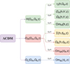 |
Fig. 1. Flowchart describing the consistency tests presented in Sect. 3. The color-coding corresponds to green for the tests that require the Hubble parameter H(z), red for those that require the angular diameter distance DA(z), yellow = red + green for tests that require both H(z) and DA(z), and finally, blue for the test that requires the luminosity distance DL(z). In all cases, we inverted or solved for crucial quantities (a process denoted by an arrow) that describe the expansion history of the Universe based on the ΛCDM model, making assumptions about the curvature as required in each test (denoted above the arrows). As an example, we can solve the Hubble parameter H(Ωm, 0, z) of ΛCDM for Ωm, 0, and assuming flatness, we can write the matter density parameter in terms of the dimensionless Hubble parameter h(z), see Eq. (11). Clearly, OmH(z)→Ωm, 0 only if ΛCDM is the correct description of the expansion of the Universe. A similar process is also followed for the remaining tests, which we can write in terms of the dimensionless distances dL(z) and dA(z). |
4. Analysis method of currently available data
4.1. Currently available data
In order to constrain deviations from the ΛCDM model and the FLRW metric, we now analyze a set of data providing information about the Hubble rate H(z), the luminosity DL(z), and the angular diameter distance DA(z). Below, we describe the currently available BAO and SNe data and present our analysis method.
We first considered the BAO data, given via measurements of the ratio dz, which is defined as
 (27)
(27)
where DV is the spherically averaged distance
![Mathematical equation: $$ \begin{aligned} D_{\rm V}(z)=\left[(1+z)^2\, D_{\rm A}^2(z)\, \frac{c\,z}{H(z)}\right]^{1/3}, \end{aligned} $$](/articles/aa/full_html/2022/04/aa42503-21/aa42503-21-eq29.gif) (28)
(28)
while rs(zd) is the comoving sound horizon at the drag epoch,
 (29)
(29)
cs(z) is the sound speed of the baryon-photon plasma, and zd is the redshift at the drag epoch; see Eq. (4) of Eisenstein & Hu (1998) for a fitting function that is accurate to about 2% on average compared to numerical estimates of rs(zd) obtained via recombination codes. Anderson et al. (2014) and Aubourg (2015) obtained similar approximations for the sound horizon that are accurate to about 0.1%, while Aizpuru et al. (2021) presented machine learning improved fitting functions, which are accurate to about 0.018%.
The actual BAO data considered here, described in terms of dz given by Eq. (27), the Hubble distance DH(z) = c/H(z), and the comoving angular diameter distance DM(z) = (1 + z) DA(z), are provided by the 6dF galaxy survey (6dFGS; Beutler et al. 2011), the WiggleZ survey (Blake et al. 2012), the third-year (Y3) data release of the dark energy survey (DES; Abbott et al. 2022), and the extended baryon oscillation spectroscopic survey (eBOSS) of the completed Sloan digital sky survey (SDSS-IV; Alam 2021). We refer to this combination of points as BAO and refer to Appendix A of Martinelli et al. (2020) and Table 3 of Alam (2021) for their exact values and their likelihood.
We have considered that a fiducial cosmology is commonly adopted in order to convert the measured angular scales into distances for the BAO data; we corrected the BAO results to be consistent with our models where necessary. However, we did not model the change in the nonlinear effects that may modify and damp the position of the BAO. This could introduce systematic uncertainties of a few percent in the reconstructions (see Angulo et al. 2008) and may lead to a lesser constraining power (see, e.g., Anselmi et al. 2018). The reason is that the BAO is essentially a feature at linear scales and the damping parameter is marginalized over. Moreover, modeling the nonlinear scales is nontrivial for theories beyond the ΛCDM model and the FLRW metric and thus is beyond the scope of this paper. Therefore, we chose not to correct for these effects and left this for future and more focused work on the subject.
We also considered the SNe, which can constrain the luminosity distance DL(z). The key observable is the apparent magnitude m(z)
![Mathematical equation: $$ \begin{aligned} m(z) = M_0+5\log _{10}{\left[\frac{D_{\rm L}(z)}{\mathrm{Mpc}}\right]}+25, \end{aligned} $$](/articles/aa/full_html/2022/04/aa42503-21/aa42503-21-eq31.gif) (30)
(30)
where M0 is the intrinsic magnitude of the supernova at a redshift z. Clearly, if no external information is provided, the Hubble constant H0 is completely degenerate with M0 as the SNe data alone cannot constrain these two quantities. Here we considered the updated Pantheon compilation of 1048 points from Scolnic et al. (2018), while for the likelihood, we used the expression given in Appendix C of Conley et al. (2011), which is already marginalized over M0 and H0 and takes the covariances of the SNe data into account.
4.2. Genetic algorithms
We now describe a machine learning approach, called genetic algorithms (GA). The GAs are a set of stochastic optimization methods that are commonly applied in the context of nonparametric reconstructions of data. They are inspired by the notion of grammatical evolution, and in particular, the genetic operations of mutation, that is, a random change in an individual, and crossover, that is, the combination of different individuals to form offspring. These operators behave as an environmental pressure, thus emulating the concept of natural selection in biology.
The reproductive success of a member of the population, or in other words, the probability that it will have offspring, is usually assumed to be proportional to its fitness, which is a measure of how accurately every member of the population fits the data. We quantified the fitness of the individuals via a standard χ2 statistic. Overall, the GA have been used to probe for extensions of the standard model (Akrami et al. 2010); deviations from ΛCDM, both at the background and the perturbation level in linear order (Nesseris & García-Bellido 2012; Arjona & Nesseris 2020a,b); to reconstruct a variety of cosmological data, such as SNe data (Bogdanos & Nesseris 2009; Arjona 2020); or to perform reconstructions of null tests, for example, the so-called Om statistic and the curvature test (Nesseris & Shafieloo 2010; Nesseris & García-Bellido 2013; Sapone et al. 2014).
We performed a simultaneous fit of the SNe and BAO data with the GA for the currently available data and for the mocks presented in later sections, via the following approach. During the initialization phase, a set of functions was randomly chosen among an orthogonal basis, in the classical sense of orthogonal polynomials for the related functions that include polynomials, exp, log, and other elementary functions, but also the operators +, −, ×, ÷, and ∧, where the wedge corresponds to exponentiation, for instance, for two functions f(x) and g(x), that would be f ∧ g ≡ fg = exp[g*log(f)], so that every member corresponds to a random guess for the Hubble rate H(z) and the luminosity distance DL(z). Although we still assumed the validity of the distance duality relation between the luminosity and angular diameter distances, DL(z) = (1 + z)2 DA(z), as this case was tested in Martinelli et al. (2020), we relaxed the assumption of Eq. (20), however, because if it is valid, then the global shear test Σ(z) is automatically satisfied regardless of the reconstruction method (GA, etc). Thus, the GA evolves the three functions of redshift that correspond to the Hubble rate H(z), the luminosity distance DL(z), and the angular diameter distance, given by DA(z) = DL(z)/(1 + z)2.
The GA does not a priori impose a prior on the functional space, and in principle, given a grammar, the output best-fitting functions are unconstrained in terms of their properties (other than they should fit the data very well). However, we do need to assume certain priors in order to ensure that the derived functions have physical meaning. The way this was done is twofold. First, we demanded that all functions were smooth, continuous, and differentiable across the redshift range covered by the data. This was done automatically in our implementation of the GA code. Second, we also assumed certain physical priors, for example, that the luminosity distance at z = 0 was zero, to ensure that the resulting functions were realistic, but we made no assumption on a DE model.
After this initial population of function was set up, we then calculated the fitness of every member via a χ2 statistic, using the SNe and BAO data and their individual covariances simultaneously as input, thus assessing the global fitness of the set of the three reconstructed functions. Next, using the tournament selection approach (see Bogdanos & Nesseris 2009 for more details), a random set of the best-fitting functions in every generation was chosen, and the crossover and mutation operators were applied to the selected functions. Finally, we iterated this process thousands of times in order to ensure a good convergence of the algorithm, but we also performed runs with different random seeds, in order to avoid biasing the results by the choice of a specific random seed.
The final output of the GA after converged is a set of three continuous and differentiable functions of redshift for the Hubble parameter H(z), the luminosity distance DL(z), and the angular diameter distance DA(z). In the case of the currently available data, we also numerically minimized the χ2 over the combination rs(zd)h, where rs(zd) is the comoving sound horizon at the drag epoch and h = H0/(100 km s−1 Mpc−1), in order to avoid any assumptions about the Hubble constant for the BAO physics at early times. However, this complication does not exist for the fiducial BAO data, as they have already been marginalized over that quantity and the angular diameter distance is directly available. Moreover, because the BAO data cannot independently constrain the combination Ωb, 0h2, we assumed the value Ωb, 0h2 = 0.02225 from Planck 2018 (Planck Collaboration VI 2020) where necessary.
The uncertainties of the best-fit Hubble parameter H(z) and the luminosity distance DL(z) were obtained from the GA via a path integral approach developed by Nesseris & García-Bellido (2012, 2013). Specifically, the uncertainties were calculated by functionally integrating the likelihood, that is, performing a path integral, over the whole functional space covered by the GA. This approach has been extensively tested by Nesseris & García-Bellido (2012) and was found to agree with error estimates obtained via a bootstrap Monte Carlo method. We used the publicly available code Genetic Algorithms for the numerical implementation of the GA1.
4.3. Binning and parameterized approach
We can now describe our parameterized method for the null tests presented in the previous section to probe for deviations from ΛCDM and spatial homogeneity. To do this, we followed a two-pronged approach.
First, we binned the Hubble rate and distance data in bins with an equal number of points, and then we calculated the various tests using the expressions in Sect. 3. The first technique to explore the sensitivity of the tests we present consists of evaluating them in redshift bins. Each test is sensitive to a particular combination of the different observables and parameters, hence the binning technique had to be performed individually to take the proper dependence and the covariances into account. To compute the OmH and r0 tests, we binned the H(z) data at different redshifts and propagated their uncertainties to the final tests by taking the diagonal elements of the covariance matrices of the data. We verified following the approach of Nesseris & Sapone (2014) that our choice of the covariance matrices did not affect the results by more than 1%.
Furthermore, to compute OmdA and OmdL, we binned the corresponding distances. DA(z) comes directly from the BAO mocks, whereas for DL(z), we used the distance moduli of SNe by inverting Eq. (30). For the distance moduli, we further binned the data in 20 equally spaced redshift bins in order to have enough points and help compute the derivatives in a wider redshift range.
The uncertainties on the final OmdL test were obtained using a standard error propagation technique. Particular care was taken for the Σ(z), Ωk(z), 𝒪m(z), and 𝒪K(z) tests. The global shear test Σ(z) depends simultaneously on H(z) and DA(z) with its first derivative with respect to redshift,  . The derivative of the angular diameter distance was obtained numerically considering two consecutive bins,
 (31)
(31)
The uncertainties on the final test were obtained by constructing the Jacobian matrix, which takes the derivatives of Σ with respect to H(z), DA(z), and  into account and by then propagating the matrix with the covariance matrix of the data.
The curvature test Ωk(z) depends on H(z), d(z) = (1 + z) c−1H0 DA(z), and d′(z), hence we recast the Ωk test as a function of the angular diameter distance in order to directly propagate the uncertainties from the data. We also adopted the numerical derivative for two consecutive bins for d′(z), similar to Eq. (31), and the final uncertainties were obtained as for the Σ(z) test.
The 𝒪m(z) and 𝒪K(z) terms only depend on H(z) and its first derivative, H′(z). The latter was evaluated numerically in the same way, and the uncertainties on the final tests were obtained using the propagation rule for both H(z) and H′(z). Finally, the number of bins for Σ(z), Ωk(z), 𝒪m(z), and 𝒪K(z) is ndata − 1 because the test depends on the first derivatives of the observables.
Second, for each of the null tests we examined, we fit the binned data we derived in the previous step with a parametric form that is inspired by the CPL parameterization for the dark energy equation of state, shown in Eq. (1), in order to obtain forecast constraints from Euclid for the deviations from the expected values and for the redshift trends of these null tests.
Specifically, each quantity we tested (P) was parameterized with the functional form
 (32)
(32)
where P0 is its value today and P1 the first derivative, both evaluated at a = 1. This simple parameterization, based on a Taylor expansion, allows us to characterize in a simple and model-independent fashion how Euclid will be able to carry out the tests. The only exception to this form is the one chosen for the test of Eq. (25), for which we multiplied the parameterization above by a factor z2 in order to ensure that there is no divergence at the present time.
Using the binned values we obtained in the first step of this approach as input data, we fit the predictions given by Eq. (32), sampling the two free parameters through the publicly available sampler Cobaya (Torrado & Lewis 2021), which exploits the Metropolis-Hastings algorithm presented in Lewis & Bridle (2002) and Lewis (2013). In each case, we assumed flat priors on the two free parameters of the analysis. The results of this parameterized approach is denoted PA below.
We emphasize that the order of the expansion we used for the PA is somewhat arbitrary. We chose to truncate the expansion at first order, analogously with the CPL parameterization for the DE equation of state, but this choice has significant effects. Our results clearly show (see Sect. 7), the PA at first order lacks the flexibility to accurately reconstruct several of the tests considered in this paper, especially when we do not consider the ΛCDM fiducial. The purpose of the PA here therefore is to perform a comparison with the GA, which clearly shows the trade-off between simplicity and accuracy of the reconstruction.
5. Analysis method for the mock data
5.1. Fiducial cosmologies
In order to forecast the ability of Euclid to improve upon the sensitivity of the null tests mentioned in Sect. 3, we relied on mock data based on a priori known fiducial cosmologies, which we briefly describe. In particular, we used the ΛCDM model, the CPL model (w0waCDM), and the ΛLTB model to create simulated data sets for the SNe and the BAO measurements based on the Euclid specifications.
First, for the fiducial cosmologies based on the ΛCDM and CPL models, we used the values of the parameters shown in Table 1. Both of these fiducial cosmologies assume no violation of the spatial homogeneity and isotropy of the FLRW metric, and the ΛCDM fiducial was also used in EC20. In this case, we can jointly write the Hubble expansion rate at late times when we safely neglect radiation and assuming flatness (Ωk, 0 = 0) for the two models as
![Mathematical equation: $$ \begin{aligned} \frac{H^2(a)}{H^2_0}=\Omega _{\rm m,0}\;a^{-3}+(1-\Omega _{\rm m,0})\; \exp \left[-3\int _1^a\frac{1+{ w}(\alpha )}{\alpha }\; \mathrm{d}\alpha \right], \end{aligned} $$](/articles/aa/full_html/2022/04/aa42503-21/aa42503-21-eq36.gif) (33)
(33)
Parameter values for the fiducial models we used for the mocks.
where the dark energy equation of state for the CPL model follows Eq. (1), which includes the ΛCDM model for (w0, wa) = (−1, 0), while the scale factor is a = 1/(1 + z). For the CPL fiducial, we chose the parameters (w0, wa) = (−0.8, −1) as an extreme case, which corresponds to the combination TT, TE, EE+lowE+lensing+SNe+BAO; see Fig. 30 of Planck Collaboration VI (2020). Furthermore, we also assumed the values for the SNe absolute magnitude M0, the baryon density Ωb, 0h2, and the Hubble rate today H0 as given in Table 1.
Regarding the ΛLTB mock, considering the LTB metric of Eq. (2) and using Einstein’s equations, we obtain the modified Friedmann equation,
![Mathematical equation: $$ \begin{aligned} H_\bot ^2(r,t) \equiv \left[\frac{\dot{R}(r,t)}{R(r,t)}\right]^2 = \frac{2m(r)}{R^3(r,t)}+\frac{2 r^2k(r)\,M^2}{R^2(r,t)}+\frac{\Lambda \; c^2}{3}, \end{aligned} $$](/articles/aa/full_html/2022/04/aa42503-21/aa42503-21-eq37.gif) (34)
(34)
where the dot is a time derivative, and the radial dependent matter density
 (35)
(35)
where M is an arbitrary mass scale, and m(r) is the so-called Euclidean mass function. We have conveniently recast K(r)≡ − 2r2k(r)M2, where k(r) is the curvature profile of the model2. In addition to the mass function, m(r), and the curvature profile, k(r), the LTB solution introduces another free function: the so-called Big Bang function, tBB(r), which appears as the constant of integration of Eq. (34), defined via
 (36)
(36)
We also assumed the compensated curvature profile,
 (37)
(37)
![Mathematical equation: $$ \begin{aligned}&P_{n}(x) = {\left\{ \begin{array}{ll} 1-\exp \left[-\frac{1}{x}(1-x)^n\right]&0 \le x < 1, \\ 0&1\le x, \end{array}\right.} \end{aligned} $$](/articles/aa/full_html/2022/04/aa42503-21/aa42503-21-eq41.gif) (38)
(38)
where kb and kc are the curvature outside and at the center of the spherical inhomogeneity, respectively, and rB is the comoving radius of the inhomogeneity. In order to avoid the decaying modes on the matter density field, we set the Big Bang function to tBB(r) = 0. The absence of decaying modes of the ΛLTB model ensures the agreement with the standard scenario of inflation. The remaining arbitrary function, m(r), is effectively a gauge choice, which we fixed here by m(r) = 4πM2r3/3 (see Biswas et al. 2010 for more details).
Since we assumed a compensated model, the ΛLTB model becomes exactly ΛCDM at scales r > rB. It is specified by the six usual ΛCDM parameters plus the parameters introduced by the profile k(r), namely kc and rB (from Eq. (34), note that kb ≡ 4πΩk, 0/3Ωm, 0). Following Camarena et al. (2021), we mapped kc into the central density contrast δ0 ≡ ρm(0, t0)/ρm(rB, t0)−1 and rB into its corresponding redshift zB. We provide the relevant parameters used for the ΛLTB mocks in Table 1, and in Fig. 2 we show the matter density contrast, defined as δρm ≡ ρm(r, t0)/ρm(rB, t0)−1. The values of the parameters δ0 and zB were chosen for historical reasons. An underdensity of contrast ≈ − 0.5 up to a redshift of ≈0.7 can indeed fit the luminosity-distance-redshift relation of the ΛCDM model, explaining away dark energy (Marra & Notari 2011).
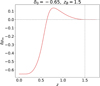 |
Fig. 2. Matter density contrast of the ΛLTB model as a function of redshift z for δ0 = −0.65 and zB = 1.5. |
After establishing the three cosmologies that we wished to examine, we calculated the fiducial background quantities for the Hubble rate, the luminosity, and angular diameter distances as a function of redshift z. Finally, using the specifications of forthcoming surveys as described below, we created our mock BAO and SNe data.
While high precision is expected from forthcoming surveys such as Euclid, it is crucial to ensure that they are accurate, and several efforts have been made to take observational systematic uncertainties into account that will affect the surveys. For example, in Euclid Collaboration (2020), the observational systematic effects of the Euclid VIS instrument were studied, also taking the modeling of the point spread function and the charge transfer inefficiency into account. While some of the specifications for future instruments might still change prior to completion, here we assumed that by the time the data arrive, the systematic effects described above will be well understood. Thus, we added all the relevant astrophysical systematic effects, such as the galaxy bias, as described in the following subsections.
Finally, it is worth stressing that the covariance matrices were computed assuming the fiducial ΛCDM cosmology. This means that we neglect the error due to the use of a non-ΛCDM fiducial cosmology. The computation of covariance matrices for alternative cosmologies is indeed an open issue in the exploitation of next-generation survey data (Harnois-Deraps et al. 2019; Friedrich et al. 2021).
5.2. SNe surveys
We considered two future SNe surveys, one based on the proposed Euclid DESIRE survey (Laureijs et al. 2011; Astier et al. 2014), and the other based on the specifications of the LSST. We assumed that the Euclid DESIRE survey will observe 1700 supernovae in the range z ∈ [0.7, 1.6], while the LSST survey will observe 8800 supernovae in the redshift range z ∈ [0.1, 1.0] for a total of 10 500 data points.
In both cases we assumed the redshift distributions described in Astier et al. (2014), and we further assumed that they are uncorrelated with each other. While the DESIRE survey is not a guaranteed output of Euclid, we include it here in order to extend the redshift range of LSST, as this is crucial for the GA reconstruction at high z. For every SNe event, we assumed an observational error of the form
 (39)
(39)
where the flux, scatter, and intrinsic contributions are the same for each event: σflux = 0.01, σscat = 0.025, and σintr = 0.12, respectively (see Astier et al. 2014). We also included an error on the distance modulus μ = m − M0 that evolves linearly with the redshift z as
 (40)
(40)
where we assumed that the parameter eM is drawn from a Gaussian distribution with zero mean and standard deviation σ(eM) = 0.01 (see Gong et al. 2010; Astier et al. 2014). The distance modulus error takes the possible redshift evolution of SNe into account, which has not been accounted for by the distance estimator; see Astier et al. (2014). We note that eM = 0.01 is needed to allow for systematic evolution, but it would just add in quadrature to the effective eM = 0.055 coming from lensing, to make a single effective eM that is negligibly different from 0.055.
The uncertainty due to lensing was estimated theoretically to be σlens = 0.052 z (Marra et al. 2013; Quartin et al. 2014) and σlens = 0.056 z (Ben-Dayan et al. 2013), and observationally with Supernova Legacy Survey data to be σlens = (0.055 ± 0.04) z (Jonsson et al. 2010) and σlens = (0.054 ± 0.024) z (Kronborg et al. 2010).
5.3. Large-scale structure surveys
As we are interested in forecasting the sensitivity of the null tests for ΛCDM with Euclid, we now describe how we simulated BAO data using the Fisher matrix approach. To do this, we followed the same method as was used in EC20 for the spectroscopic survey.
We mainly focus on the spectroscopic Euclid survey because our goal is to obtain precise measurements of the Hubble parameter H(z) and the angular diameter distance DA(z). Overall, the Euclid survey will be able to probe the galaxy power spectrum in the redshift range z ∈ [0.9, 1.8] where, as mentioned in EC20, the main targets are Hα emitters. In this case, Euclid will measure up to 30 million spectroscopic redshifts with an uncertainty given by σz = 0.001(1 + z) (Pozzetti et al. 2016) and the main observable will be the galaxy power spectrum. This power spectrum carries information about the distortions due to the Alcock-Paczynski effect, the residual shot noise, the redshift uncertainty, and the anisotropies due to redshift space distortions and on the galaxy bias. Moreover, nonlinear effects that distort the shape of the power spectrum, for instance, a nonlinear smearing of the BAO feature, were also included in the matter power spectrum (Wang et al. 2013). In principle, other effects might also include a nonlinear scale-dependent galaxy bias;d see for example de la Torre & Guzzo (2012).
We use the same binning scheme as in Martinelli et al. (2020), which is different from that of EC20; specifically, we used nine equally spaced redshift bins of width Δz = 0.1 instead of four. By rebinning the data as given in EC20, we find the following specifications for the galaxy number density n(z) in units of Mpc−3 and the galaxy bias b(z),

This binning scheme allows for more data points and considerably improves the machine learning analysis, as discussed below. However, we note that we tested this particular choice against that of EC20 in Martinelli et al. (2020), where we found no statistically significant difference.
In order to obtain the Fisher matrix for the full set of cosmological parameters, which is used to estimate the parameter covariance matrix and propagate the error estimates, we followed the procedure described in EC20. The analysis includes the following parameters: the four shape parameters {ωm = Ωm, 0h2, h, ωb = Ωb, 0h2, and ns}, the two nonlinear parameters {σpand σv} (see EC20), and the five redshift-dependent parameters {lnDA, lnH, lnfσ8, lnbσ8, and Ps}, evaluated in each redshift bin, where fσ8 ≡ f(z)σ8(z) is the linear growth rate times σ8, which measures the amplitude of the linear power spectrum at scales of 8h−1 Mpc, while bσ8 ≡ b(z)σ8(z) and Ps characterize the galaxy bias and the shot noise, respectively (see EC20). In this way, we can derive the expected uncertainties from the Euclid survey of the Hubble parameter H(z) and the angular diameter distance DA(z) in each of the nine redshift bins, while we marginalize over all the other parameters. The final Fisher matrix in principle depends on the particular fiducial cosmology, but here we assumed that this dependence is weak at best.
As the Euclid spectroscopic survey will only probe the redshift range z ∈ [0.9, 1.8], we will be limited in the range in which both BAO and the SNe data are available. Thus, we complemented our analysis by including the DESI survey, in order to be able to reconstruct the null tests at the full range of the available SNe data. DESI has started survey operations in 2021 and is scheduled to obtain optical spectra for tens of millions of quasars and galaxies up to z ∼ 4, which will allow BAO and redshift-space distortion analyses.
We followed the official DESI forecasts for the Hubble parameter H(z) and the angular diameter distance DA(z) as described in DESI Collaboration (2016). These forecasts have also been derived following a Fisher matrix approach, described in Font-Ribera et al. (2014), which is the full anisotropic galaxy power spectrum, that is, measurements of the matter power spectrum as a function of the angle with respect to the line of sight, but also redshift and wavenumber. Similarly to the Euclid forecasts, this approach also includes all the available information from the two-point correlation function and not just the position of the BAO peak.
Specifically, we considered the baseline DESI survey, covering 14 000 deg2 and targeting bright galaxies (BGs), luminous red galaxies (LRGs), emission-line galaxies (ELGs), and quasars in the redshift range z ∈ [0.05, 3.55], but with a precision that will explicitly depend on the target population. First, the BGs will be in the redshift range z ∈ [0.05, 0.45] given in 5 equally spaced redshift bins, while the next two targets, the LRGs and ELGs, will be in the range z ∈ [0.65, 1.85] in 13 equally spaced redshift bins. Moreover, the Ly-α forest quasars will be given in the range z ∈ [1.96, 3.55] in 11 equally spaced redshift bins. Finally, we assumed that these measurements are not correlated with each other.
In our analysis we only included the DESI data at late times that do not overlap the Euclid points in order to avoid spurious correlations between the two surveys. Furthermore, as the SNe data from LSST + DESIRE will only reach redshift z = 1.6, we only included the DESI data from the full BGs survey and the LRGs and ELGs up to z = 0.9, thus leaving out the Ly-α forest observations.
6. Results from the current data
In this section we now present the reconstructions of the null tests of Sect. 3 using the currently available SNe and BAO data. In this case, as the BAO data are coming from a plethora of different surveys and in a variety of different forms, that is, in terms of dz(z), 1/dz(z), and so on, we cannot bin them without introducing new assumptions on their statistical properties. Thus, we only present the results of the GA analysis, following the method presented in Sect. 4.2. In order to simplify the discussion of the results, we split the tests into groups of related tests.
Specifically, we show in Fig. 3 the GA reconstructions of the null tests. In the first row from the top of Fig. 3 we show the GA reconstructions of the two tests for the matter density, which directly probe the Hubble expansion rate, namely OmH(z) given by Eq. (11) (left) and 𝒪m(z) given by Eq. (12) (right). They agree with a constant value and the ΛCDM within the 68% uncertainties, but 𝒪m(z) is closer to the 68% confidence level boundary because of the presence of the derivatives of the Hubble parameter, which amplify any deviations from the concordance value; see Eq. (12).
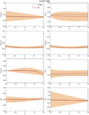 |
Fig. 3. GA reconstructions of the null tests mentioned in Sect. 3 using the currently available BAO and Pantheon SNe data, as described in Sect. 4. In all cases, the dashed line at zero corresponds to the best-fit ΛCDM model, described by Eq. (10) and the parameters (Ωm, 0 = 0.303, h = 0.659), the red line is the GA fit, and the orange shaded region corresponds to the 68% GA uncertainties. |
In the second row from the top, we show the reconstructions for the matter density tests that directly probe the cosmological distances, namely OmdL(z) given by Eq. (22) (left panel) and OmdA(z) given by Eq. (24) (right panel). They also agree well with a constant value and the ΛCDM best fit within the errors. Next, in the third row from the top, we show the two curvature tests that probe the spatial homogeneity of the Universe, namely z2Ωk(z) given by Eq. (25) (left panel) versus 𝒪K(z) given by Eq. (13) (right panel). In this case, both tests are consistent with a flat universe at the 68% confidence level, but the uncertainties seem to increase with redshift for the z2Ωk(z) due to the additional z2 term, which suppresses the singularity at late times, as explained in Sect. 3. On the other hand, 𝒪K(z) is closer to the 68% confidence level boundary because it is complementary to 𝒪m(z) and is subject to the same impact of the presence of the Hubble derivative in their expression.
Furthermore, in the bottom row, we show the global shear test Σ(z) (left panel) given by Eq. (19), which tests the Copernican principle, and the r0(z) null test (right panel), which probes for dark matter-dark energy interactions and is given by Eq. (17). Again, both tests are consistent within the uncertainties with the assumption of the Copernican principle and no interactions in the dark sector. In some cases, for instance, in the OmH(z) and the r0(z) tests, the error regions increase at low redshifts because these tests are ill defined in the zero redshift limit, as discussed in Sect. 3. Similarly, this also occurs for the z2Ωk(z) test, but because of the additional z2, which regularizes the singularity at z = 0, it now instead occurs at high redshifts.
Finally, as the GA does not to evaluate the statistical significance of a potential departure from the ΛCDM in a straightforward fashion, we also implemented a quantitative approach of estimating the average deviation from the null hypothesis and the average size of the errors across the redshift range of the data. We also present the results of the mock data below, and then this approach is particularly useful because it allows us to obtain an overall improvement factor that forthcoming surveys will add when they are compared to the current data of this section. The technical details of this analysis are given in Appendix A.
7. Forecast results
Following the approach described in Sect. 5, we now present the constraint estimates of our null tests using the SNe and BAO mock data for three different fiducial cosmologies based on the vanilla flat ΛCDM model given by Eq. (10), the CPL parameterization given by Eq. (1), and the ΛLTB model described by Eq. (34), assuming the fiducial values for the parameters shown in Table 1. In our analysis we also consider two different cases. In the first case, we only use the Euclid BAO data, spanning the range z ∈ [0.9, 1, 8], in order to quantify the ability of the Euclid survey alone to constrain any deviations from the null tests. In a second case, we also include the DESI BAO data, which cover the lower redshifts, as discussed in Sect. 5, in order to highlight the synergies of the two surveys. Both cases include all SNe data (Euclid + LSST), and similarly to Sect. 6, we group the plots by row, splitting the tests into groups of related tests.
As in this case the mock BAO data are always given in terms of the angular diameter distance DA(z) and the Hubble expansion rate H(z), we are now also able to perform the binning analysis as discussed in Sect. 4.3 as a model-independent analysis complementary to that of the GA. The binned data produced by this approach are also used to obtain constraint estimates on the considered tests, using a parametric approach based on a CPL-like parameterization given by Eq. (32). However, that while we apply the GA simultaneously to the full SNe and BAO mock data, the PA is only applied on the binned data of each test.
Finally, as mentioned in the previous section, we also implement a quantitative approach of estimating the overall improvement factors that are expected from forthcoming surveys when compared to the current data of the previous section. The technical details of this analysis are given in Appendix A.
7.1. Results from the ΛCDM mocks
First, we present in Fig. 4 the results of the GA reconstructions of the null tests described in Sect. 3 for the Euclid-only ΛCDM mocks and in Fig. 5 for all mock data (Euclid + DESI). In all cases, both here and in the plots below, the dashed line corresponds to the fiducial value of the test under consideration for ΛCDM, the red line is the GA fit, the blue line is the PA fit given by Eq. (32) of the binned mock data (black points), while the orange and blue shaded regions correspond to the 68% uncertainties of the GA and PA, respectively, and the vertical dashed line at z = 0.9 indicates the minimum redshift of the Euclid-only points. Because the binned mock data include a random realization of error, they are expected to fluctuate around the fiducial value. This is indeed seen in Figs. 4 and 5.
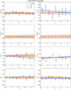 |
Fig. 4. GA reconstructions of the null tests mentioned in Sect. 3 using the Euclid-only BAO and Euclid + LSST SNe ΛCDM mock data. In all cases, the dashed line corresponds to the fiducial value of the corresponding test for ΛCDM, the red line is the GA fit, the blue line is the PA fit, the shaded regions correspond to the 68% uncertainties, and the black points correspond to the binned Euclid mock data. |
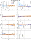 |
Fig. 5. GA reconstructions of the null tests mentioned in Sect. 3 using the Euclid + DESI BAO and Euclid + LSST SNe ΛCDM mock data. In all cases, the dashed line corresponds to the fiducial value of the corresponding test for ΛCDM, the red line is the GA fit, the blue line is the PA fit, the shaded regions correspond to the 68% uncertainties, and the black points correspond to the binned Euclid and DESI mock data. The vertical dashed line at z = 0.9 indicates the minimum redshift of the Euclid-only points. |
All of the panels of Fig. 4 show that in all cases, both the GA and the PA reconstructions along with the binned mock data are able to correctly predict the fiducial model to within the 95% uncertainties. Because of their agnostic nature, the uncertainties of the GA reconstructions (orange shaded regions) are somewhat larger than those of the PA (blue shaded regions), but they are very similar to those of the binning (black points). An exception to this is the OmdA(z) test, which in the case of the GA is dominated by the systematic uncertainties of the SNe data because of the joint reconstruction approach employed in this case, as was also observed in Martinelli et al. (2020). In particular, as we fit all the data (SNe and BAO) simultaneously, the errors of the GA reconstructions for the distances are dominated by the measurements with the larger (worst) errors, which in this case are the SNe. Hence, using the GA reconstructions for the angular diameter distance results in much larger errors than in the PA method. The PA method does not suffer from this issue as the PA fits the Taylor expansion directly only to the binned BAO angular diameter data.
On the other hand, when we also include the DESI BAO data at low and intermediate redshifts that do not overlap the Euclid points, as shown in Fig. 5, we find that the uncertainties in the case of the binning approach dramatically increase because the constraining power of DESI is lower than that of Euclid at this redshift range. This affects the PA (blue shaded regions), as in some cases, such as for the Σ(z) and the 𝒪K(z) tests, it misses the fiducial model (dashed line) by more than 1σ. The reason for this is that the PA is anchored to the Euclid points at intermediate redshifts, which have smaller error bars than the Euclid redshifts, and because the PA parameterization lacks flexibility, discrepancies appear at low redshifts. This also affects the GA reconstruction for Σ(z), but in the remaining cases, the GA efficiently predicts the correct cosmology as it uses the full SNe and BAO data. In either case, these deviations are due to the presence of derivatives in the null tests, which tend to cause instabilities in the reconstructions.
Overall, after analyzing the ΛCDM mocks, we find that Euclid, in combination with other surveys, will be able to improve current constraints by approximately a factor of three with the machine learning approach. The binning and parametric approach will provide an improvement of a further factor of two over the GA results.
7.2. Results from the CPL mocks
Next, we present in Fig. 6 the results of the GA and parametric reconstructions of the null tests for the Euclid-only CPL mocks. In Fig. 7 we show them for all mock data (Euclid + DESI).
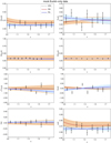 |
Fig. 6. GA reconstructions of the null tests mentioned in Sect. 3 using the Euclid-only BAO and Euclid + LSST SNe data for the CPL mock for (w0, wa) = (−0.8, −1). In all cases, the dashed line corresponds to the fiducial value of the corresponding test for CPL, the red line is the GA fit, the blue line is the PA fit, the shaded regions correspond to the 68% uncertainties, and the black points correspond to the binned Euclid mock data. |
This case now is more interesting because the nature of the DE model we chose means that many of the tests that probe the expansion history of the Universe, such as the OmH(z), have a distinct evolution with redshift. In the case of the Euclid-only mocks shown in Fig. 6, both approaches overall predict the fiducial cosmology within the errors, but in some cases, there is a small 1σ deviation. This occurs, for example, in the case of the OmH(z) test with the GA because the GA cannot anchor very well at z ∼ 1 because it lacks points at low redshift. On the other hand, in the case of the binning, for the 𝒪m(z) and 𝒪K(z) tests, the presence of derivatives in the expressions causes more scatter in the points, which is also propagated to the PA (blue line). This also affects the r0(z) test, where the effect is further amplified by the need to fix the baryon density parameter Ωb, 0 to its Planck best-fit value.
When we also include the DESI BAO data, see Fig. 7, we can extend the reconstructions of the tests to low redshifts, where many of the tests, such as the fiducial value of the OmH(z) test, manifest large deviations from a constant value. In this case, we find that while the GA follows the fiducial trend quite well, the PA (blue line) is anchored to the higher redshift Euclid points, as these have smaller uncertainties than the DESI points, and it deviates from the fiducial model by several σ; a similar effect is also visible for the r0(z) test. Finally, neither in Euclid-only nor in Euclid + DESI BAO data is the global shear test affected as expected, and the reconstructions are practically identical to the reconstruction of the ΛCDM mocks.
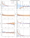 |
Fig. 7. GA reconstructions of the null tests mentioned in Sect. 3 using the Euclid + DESI BAO and Euclid + LSST SNe data for the CPL mock for (w0, wa) = (−0.8, −1). In all cases, the dashed line corresponds to the fiducial value of the corresponding test for CPL, the red line is the GA fit, the blue line is the PA fit, the shaded regions correspond to the 68% uncertainties, and the black points correspond to the binned Euclid and DESI mock data. The vertical dashed line at z = 0.9 indicates the minimum redshift of the Euclid-only points. |
7.3. Results from the ΛLTB mocks
Finally, we now present in Fig. 8 the results of the GA and PA for the Euclid-only ΛLTB mocks and in Fig. 9 for all mock data (Euclid + DESI). This particular case is even more interesting, as all the tests present large deviations compared to the simple ΛCDM case. This is due to the void profile we used. Specifically, when compared to the corresponding plots for the ΛCDM mocks, the ΛLTB mocks exhibit large deviations from a constant value at small redshifts, due to the shape of the void profile, in particular in the cases of OmH(z), r0(z), 𝒪m(z) and 𝒪K(z).
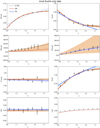 |
Fig. 8. GA reconstructions of the null tests mentioned in Sect. 3 using the Euclid-only BAO and Euclid + LSST SNe data for the ΛLTB mock. In all cases, the dashed line corresponds to the fiducial value of the corresponding test for the ΛLTB model, the red line is the GA fit, the blue line is the PA fit, the shaded regions correspond to the 68% uncertainties, and the black points correspond to the binned Euclid mock data. |
Fig. 8 shows that in the case of the Euclid-only BAO data, the PA given by Eq. (32) is not flexible enough to reproduce the fiducial model; see, for example, the top left panel of Fig. 8 for the OmH(z) reconstruction or the OmdL(z) and OmdA(z) tests in the second row. The latter actually give very high values of the matter density. This would be a smoking gun for the presence of voids. In the case of the 𝒪K(z) test, the GA is much closer to the fiducial model than to the PA, while for the r0(z) test, the deviation is again partly due to fixing the value of the baryon density, as before. When we also include the DESI BAO data, the reconstructions of Fig. 9 clearly highlight the ability of our approach to fully harness the power of the null tests of Sect. 3.
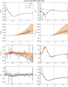 |
Fig. 9. GA reconstructions of the null tests mentioned in Sect. 3 using the Euclid + DESI BAO and Euclid + LSST SNe data for the ΛLTB mock. In all cases, the dashed line corresponds to the fiducial value of the corresponding test for the ΛLTB model, the red line is the GA fit, the blue line is the PA fit, the shaded regions correspond to the 68% uncertainties, and the black points correspond to the binned Euclid and DESI mock data. The vertical dashed line at z = 0.9 indicates the minimum redshift of the Euclid-only points. |
In particular, because of the choice of the ΛLTB profile, several of the tests, namely OmH(z), 𝒪K(z), r0(z), and Σ(z), have large deviations from a constant value, which the GA is able to capture correctly. The simultaneous fitting of the data with the GA, see Sect. 4.2, causes some correlations between the Hubble parameter and the luminosity distance, however. As a result, the fits in the redshift range covered by Euclid might differ between the Euclid-only and Euclid + DESI cases because of the added DESI BAO data at low z in the latter case, which may shift the fit. This difference in the fits between the two data sets can be seen, for example, in the OmdL(z) test shown in Fig. 8 and Fig. 9 for the two sets of mocks.
On the other hand, in these cases, the PA is again anchored at high redshifts because the uncertainties of the Euclid data are small, and because of its simple redshift evolution, it misses the features at small z. The same but in the opposite direction occurs for the reconstructions of the OmdL(z) and OmdA(z) tests, but in this case, the GA and the parametric approach are always within the errors.
8. Conclusions
We have constrained deviations from the Copernican principle, the spatial homogeneity of the Universe on large scales, and from the ΛCDM model using a set of null tests, that is, identities that have to be equal to a constant value at all redshifts, using current and forecast data. For the latter, we mainly focused on the constraints coming from synergies between Euclid and other surveys, namely DESI and LSST, using BAO and SNe data.
In Sect. 2 we presented several mechanisms for which fundamental assumptions of the standard cosmological model, such as spatial homogeneity and the Copernican principle, may break down, as in the case of Bianchi or LTB models, for instance. For this reason, we employed two theory-agnostic reconstruction approaches, one approach based on machine learning, called the GA, and another based on binning the data and then fitting a simple CPL-like parameterization, which we called the PA. These approaches allowed us to derive constraints on any deviation from the standard model with only a few assumptions on the redshift trends of these deviations. Avoiding any further assumptions is particularly important as assuming a particular model and then fitting the data introduces theoretical biases, and as we have shown, makes it prone to misinterpreting deviations from the standard model.
In order to probe for deviations from the Copernican principle, the spatial homogeneity of the Universe on large scales, and from the ΛCDM model we used a set of null tests proposed over the years in the literature, which we summarized in Sect. 3. These tests probe different aspects of the aforementioned assumptions and provide a holistic approach to quantifying whether we might be able to detect any deviations from them.
We first considered the currently available SNe and BAO data. Using the GA, we found that within the errors, all the tests are compatible with the null hypothesis, that is, there were no deviations from the assumptions of the standard cosmological model, see Sect. 6 and Fig. 3. This is to be expected to some extent because the uncertainties of the currently available SNe and BAO data are large, which makes it difficult to detect any trends in the underlying cosmological model.
The fact that our current constraints are limited by the available BAO data highlights the importance of future full-sky surveys, such as Euclid. Thus, we considered mock data based on the specifications of Euclid and also allowed for synergies with DESI and LSST, in order to forecast deviations from the assumptions of the standard cosmological model for three different fiducial cosmologies: one cosmology based on the ΛCDM model, one based on the CPL model for parameters at the 95% limit of the current Planck best-fit, and finally, another mock based on the ΛLTB model, which describes an inhomogeneous universe with a cosmological constant, as described in Sect. 5.
Performing a simultaneous fit of these mock SNe and BAO data with the GA, we found, using the quantitative method described in Appendix A, an improvement of a factor of three in each case over the current constraints for most of the consistency tests, assuming the ΛCDM mocks, as seen in Table A.1. Alongside the GA, we also applied the PA, which relies on the choice of a parameterization for the trend in redshift of the tests. Overall, we find that the GA provides larger errors than the PA, and this is for two main reasons. First, the GA is a nonparametric approach, thus is more agnostic, and it spans or explores the much larger functional space, instead of just the usual parameter space as in MCMCs. This tends to increase the errors; see Nesseris & García-Bellido (2012).
Second, the choice of a parameterization for the PA creates a lack of flexibility, which is particularly evident in the cases of the CPL and ΛLTB mocks. This results in reconstructions that deviate significantly from expectations. This lack of flexibility also results in error bars that are tighter than those of the GA because the posterior of PA parameters drops sharply moving away from their best fit. These issues can in principle be avoided by increasing the flexibility of the PA, for example, considering higher-order redshift terms in Eq. (32). However, in realistic situations, the degree of complexity needed for the reconstruction would be unknown, and we decided here to use a common way to parameterize a redshift trend. This stresses even more strongly the advantage of the GA, which does not require any a priori assumption to obtain the required level of flexibility.
Finally, we limited our analysis to the ΛCDM, CPL, and ΛLTB because it is currently not feasible to go beyond these models, for example, by considering extensions such as the Bianchi type-I or back-reaction models. We lack validated codes that might be used to estimate the necessary functions (distances and expansion rates). It is therefore quite difficult to test the response of our null tests to these extensions of the standard cosmological model, but with new developments in theoretical model simulation, we could explore them in the future.
In summary, this work highlights the benefits of synergies between the Euclid BAO survey and external probes in constraining any deviations from the fundamental assumptions of the standard cosmological model. In particular, we have demonstrated that such a BAO survey will make it possible to constrain deviations from the Copernican principle, the spatial homogeneity of the Universe, and the ΛCDM model at an unprecedented level in the near future using both non-parametric and parameterized approaches.
Here, H⊥ and M have units of Mpc−1, m has units of Mpc, and that k(r) is dimensionless.
Acknowledgments
We are grateful to S. Ávila for interesting discussions. J.G.B., M.M. and S.N. acknowledge support from the research project PGC2018-094773-B-C32, and the Centro de Excelencia Severo Ochoa Program SEV-2016-059. S.N. also acknowledges support from the Ramón y Cajal program through Grant No. RYC-2014-15843. M.M. also received support from “la Caixa” Foundation (ID 100010434), with fellowship code LCF/BQ/PI19/11690015. D.S. acknowledges financial support from the Fondecyt Regular project number 1200171. The work of CJM was financed by FEDER – Fundo Europeu de Desenvolvimento Regional funds through the COMPETE 2020 – Operational Programme for Competitiveness and Internationalisation (POCI), and by Portuguese funds through FCT – Fundação para a Ciência e a Tecnologia in the framework of the project POCI-01-0145-FEDER-028987. D.C. thanks CAPES for financial support. V.M. thanks CNPq and FAPES for partial financial support. L.L. was supported by a Swiss National Science Foundation (SNSF) Professorship grant (No. 170547). This project has received funding from the European Union’s Horizon 2020 research and innovation programme under the Marie Sklodowska-Curie grant agreement No 888258. C.C. is supported by the UK Science and Technology Facilities Council (STFC) Consolidated Grant ST/P000592/1. A.dS. acknowledges support from the Fundação para a Ciência e a Tecnologia (FCT) through the Investigador FCT Contract No. IF/01135/2015 and POCH/FSE (EC) and in the form of an exploratory project with the same reference. J.P.M. and A.dS. acknowledge support from FCT Projects with references EXPL/FIS-AST/1368/2021, PTDC/FIS-AST/0054/2021, UIDB/04434/2020, UIDP/04434/2020, CERN/FIS-PAR/0037/2019, PTDC/FIS-OUT/29048/2017. Z.S. acknowledges support from the IRAP and IN2P3 Lyon computing centers. P.F. received the support of a fellowship from “la Caixa” Foundation (ID 100010434). The fellowship code is LCF/BQ/PI19/11690018. I.T. acknowledges support from the Spanish Ministry of Science, Innovation and Universities through grant ESP2017-89838, and the H2020 programme of the European Commission through grant 776247. The Euclid Consortium acknowledges the European Space Agency and a number of agencies and institutes that have supported the development of Euclid, in particular the Academy of Finland, the Agenzia Spaziale Italiana, the Belgian Science Policy, the Canadian Euclid Consortium, the Centre National d’Etudes Spatiales, the Deutsches Zentrum für Luft-und Raumfahrt, the Danish Space Research Institute, the Fundação para a Ciência e a Tecnologia, the Ministerio de Economia y Competitividad, the National Aeronautics and Space Administration, the Netherlandse Onderzoekschool Voor Astronomie, the Norwegian Space Agency, the Romanian Space Agency, the State Secretariat for Education, Research and Innovation (SERI) at the Swiss Space Office (SSO), and the United Kingdom Space Agency. A complete and detailed list is available on the Euclid web site (http://www.euclid-ec.org).
References
- Abbott, T. M. C., Aguena, M., Allam, S., et al. 2022, Phys. Rev. D, 105, 043512 [CrossRef] [Google Scholar]
- Aizpuru, A., Arjona, R., & Nesseris, S. 2021, Phys. Rev. D, 104. 043521 [CrossRef] [Google Scholar]
- Akrami, Y., Scott, P., Edsjo, J., Conrad, J., & Bergstrom, L. 2010, J. High Energy Phys., 04, 057 [CrossRef] [Google Scholar]
- Alam, S., Aubert, M., Avila, S., et al. 2021, Phys. Rev. D, 103, 083533 [NASA ADS] [CrossRef] [Google Scholar]
- Albrecht, A., Bernstein, G., Cahn, R., et al. 2006, ArXiv e-prints [arXiv:astro-ph/0609591] [Google Scholar]
- Alnes, H., Amarzguioui, M., & Gron, O. 2006, Phys. Rev. D, 73, 083519 [NASA ADS] [CrossRef] [Google Scholar]
- Alonso, D., Salvador, A. I., Sánchez, F. J., et al. 2015, MNRAS, 449, 670 [NASA ADS] [CrossRef] [Google Scholar]
- Amendola, L., Appleby, S., Avgoustidis, A., et al. 2018, Liv. Rev. Rel., 21, 2 [Google Scholar]
- Andersson, L., & Coley, A. 2011, CQG, 28, 160301 [NASA ADS] [CrossRef] [Google Scholar]
- Anderson, L., Aubourg, E., Bailey, S., et al. 2014, MNRAS, 441, 24 [NASA ADS] [CrossRef] [Google Scholar]
- Angulo, R., Baugh, C., Frenk, C., & Lacey, C. 2008, MNRAS, 383, 755 [Google Scholar]
- Anselmi, S., Starkman, G. D., Corasaniti, P.-S., Sheth, R. K., & Zehavi, I. 2018, Phys. Rev. Lett., 121, 021302 [NASA ADS] [CrossRef] [Google Scholar]
- Arjona, R. 2020, JCAP, 08, 009 [CrossRef] [Google Scholar]
- Arjona, R., & Nesseris, S. 2020a, JCAP, 11, 042 [NASA ADS] [CrossRef] [Google Scholar]
- Arjona, R., & Nesseris, S. 2020b, Phys. Rev. D, 101, 123525 [CrossRef] [Google Scholar]
- Arjona, R., & Nesseris, S. 2021, Phys. Rev. D, 104, 103532 [CrossRef] [Google Scholar]
- Astier, P., Balland, C., Brescia, M., et al. 2014, A&A, 572, A80 [NASA ADS] [CrossRef] [EDP Sciences] [Google Scholar]
- Aubourg, E., et al. 2015, Phys. Rev. D, 92, 123516 [NASA ADS] [CrossRef] [Google Scholar]
- Ben-Dayan, I., Gasperini, M., Marozzi, G., Nugier, F., & Veneziano, G. 2013, JCAP, 06, 002 [CrossRef] [Google Scholar]
- Beutler, F., Blake, C., Colless, M., et al. 2011, MNRAS, 416, 3017 [NASA ADS] [CrossRef] [Google Scholar]
- Biswas, T., & Notari, A. 2008, JCAP, 06, 021 [CrossRef] [Google Scholar]
- Biswas, T., Notari, A., & Valkenburg, W. 2010, JCAP, 11, 030 [CrossRef] [Google Scholar]
- Blake, C., Brough, S., Colless, M., et al. 2012, MNRAS, 425, 405 [Google Scholar]
- Blanchard, A., Camera, S., Carbone, C., et al. 2020, A&A, 642, A191 [NASA ADS] [CrossRef] [EDP Sciences] [Google Scholar]
- Bogdanos, C., & Nesseris, S. 2009, JCAP, 05, 006 [CrossRef] [Google Scholar]
- Buchert, T. 2008, Gen. Rel. Grav., 40, 467 [NASA ADS] [CrossRef] [Google Scholar]
- Buchert, T., Carfora, M., Ellis, G. F. R., et al. 2015, CQG, 32, 215021 [NASA ADS] [CrossRef] [Google Scholar]
- Bull, P., Clifton, T., & Ferreira, P. G. 2012, Phys. Rev. D, 85, 024002 [NASA ADS] [CrossRef] [Google Scholar]
- Camarena, D., Marra, V., Sakr, Z., & Clarkson, C. 2021, MNRAS, 509, 1291 [NASA ADS] [CrossRef] [Google Scholar]
- Célérier, M.-N. 2000, A&A, 353, 63 [NASA ADS] [Google Scholar]
- Chevallier, M., & Polarski, D. 2001, Int. J. Mod. Phys. D, 10, 213 [Google Scholar]
- Chiang, H. W., Romano, A. E., Nugier, F., & Chen, P. 2019, JCAP, 11, 016 [CrossRef] [Google Scholar]
- Clarkson, C. 2012, C. R. Phys., 13, 682 [NASA ADS] [CrossRef] [Google Scholar]
- Clarkson, C., & Regis, M. 2011, JCAP, 02, 013 [CrossRef] [Google Scholar]
- Clarkson, C., Bassett, B., & Lu, T. H.-C. 2008, Phys. Rev. Lett., 101, 011301 [NASA ADS] [CrossRef] [Google Scholar]
- Clarkson, C., Ellis, G., Larena, J., & Umeh, O. 2011, Rept. Prog. Phys., 74, 112901 [NASA ADS] [CrossRef] [Google Scholar]
- Conley, A., Guy, J., Sullivan, M., et al. 2011, ApJS, 192, 1 [Google Scholar]
- Costille, A., Caillat, A., Rossin, C., et al. 2018, in Space Telescopes and Instrumentation 2018: Optical, Infrared, and Millimeter Wave, eds. M. Lystrup, H. A. MacEwen, G. G. Fazio, et al., Int. Soc. Opt. Photon. (SPIE), 10698, 730 [Google Scholar]
- Cropper, M., Pottinger, S., Azzollini, R., et al. 2018, in Space Telescopes and Instrumentation 2018: Optical, Infrared, and Millimeter Wave, eds. M. Lystrup, H. A. MacEwen, G. G. Fazio, et al., Int. Soc. Opt. Photon. (SPIE), 10698, 709 [Google Scholar]
- de la Torre, S., & Guzzo, L. 2012, MNRAS, 427, 327 [NASA ADS] [CrossRef] [Google Scholar]
- DESI Collaboration (Aghamousa, A., et al.) 2016, ArXiv e-prints [arXiv:1611.00036] [Google Scholar]
- Di Valentino, E., Mena, O., Pan, S., et al. 2021, CQG, 38, 153001 [NASA ADS] [CrossRef] [Google Scholar]
- Einstein, A., & Straus, E. G. 1945, Rev. Mod. Phys., 17, 120 [NASA ADS] [CrossRef] [Google Scholar]
- Eisenstein, D. J., & Hu, W. 1998, ApJ, 496, 605 [Google Scholar]
- Ellis, G. F. R., & MacCallum, M. A. H. 1969, Commun. Math. Phys., 12, 108 [NASA ADS] [CrossRef] [Google Scholar]
- Ellis, G. F. R., & van Elst, H. 1999, NATO Sci. Ser. C, 541, 1 [NASA ADS] [Google Scholar]
- Euclid Collaboration (Paykari, P., et al.) 2020, A&A, 635, A139 [NASA ADS] [CrossRef] [EDP Sciences] [Google Scholar]
- February, S., Larena, J., Smith, M., & Clarkson, C. 2010, MNRAS, 405, 2231 [NASA ADS] [Google Scholar]
- Font-Ribera, A., McDonald, P., Mostek, N., et al. 2014, JCAP, 05, 023 [CrossRef] [Google Scholar]
- Friedrich, O., Andrade-Oliveira, F., Camacho, H., et al. 2021, MNRAS, 508, 3125 [NASA ADS] [CrossRef] [Google Scholar]
- García-Bellido, J., & Haugboelle, T. 2008a, JCAP, 0804, 003 [CrossRef] [Google Scholar]
- García-Bellido, J., & Haugboelle, T. 2008b, JCAP, 0809, 016 [CrossRef] [Google Scholar]
- García-Bellido, J., & Haugboelle, T. 2009, JCAP, 0909, 028 [CrossRef] [Google Scholar]
- Giblin, J. T., Mertens, J. B., & Starkman, G. D. 2016, ApJ, 833, 247 [NASA ADS] [CrossRef] [Google Scholar]
- Gong, Y., Cooray, A., & Chen, X. 2010, ApJ, 709, 1420 [NASA ADS] [CrossRef] [Google Scholar]
- Green, S. R., & Wald, R. M. 2014, CQG, 31, 234003 [NASA ADS] [CrossRef] [Google Scholar]
- Harnois-Deraps, J., Giblin, B., & Joachimi, B. 2019, A&A, 631, A160 [NASA ADS] [CrossRef] [EDP Sciences] [Google Scholar]
- Heavens, A. F., Jimenez, R., & Maartens, R. 2011, JCAP, 09, 035 [CrossRef] [Google Scholar]
- Jonsson, J., Sullivan, M., Hook, I., et al. 2010, MNRAS, 405, 535 [NASA ADS] [Google Scholar]
- Kaiser, N. 2017, MNRAS, 469, 744 [NASA ADS] [Google Scholar]
- Kolb, E. W., Marra, V., & Matarrese, S. 2010, Gen. Rel. Grav., 42, 1399 [NASA ADS] [CrossRef] [Google Scholar]
- Kronborg, T., Hardin, D., Guy, J., et al. 2010, A&A, 514, A44 [NASA ADS] [CrossRef] [EDP Sciences] [Google Scholar]
- Laureijs, R., Amiaux, J., Arduini, S., et al. 2011, ArXiv e-prints [arXiv:1110.3193] [Google Scholar]
- Laurent, P., Le Goff, J.-M., Burtin, E., et al. 2016, JCAP, 11, 060 [CrossRef] [Google Scholar]
- Lewis, A. 2013, Phys. Rev. D, 87, 103529 [NASA ADS] [CrossRef] [Google Scholar]
- Lewis, A., & Bridle, S. 2002, Phys. Rev. D, 66, 103511 [Google Scholar]
- Linder, E. V. 2003, Phys. Rev. Lett., 90, 091301 [Google Scholar]
- LSST Science Collaboration (Abell, P. A., et al.) 2009, ArXiv e-prints [arXiv:0912.0201] [Google Scholar]
- Marra, V., & Notari, A. 2011, CQG, 28, 164004 [NASA ADS] [CrossRef] [Google Scholar]
- Marra, V., & Sapone, D. 2018, Phys. Rev. D, 97, 083510 [NASA ADS] [CrossRef] [Google Scholar]
- Marra, V., Kolb, E. W., Matarrese, S., & Riotto, A. 2007, Phys. Rev. D, 76, 123004 [NASA ADS] [CrossRef] [Google Scholar]
- Marra, V., Quartin, M., & Amendola, L. 2013, Phys. Rev. D, 88, 063004 [NASA ADS] [CrossRef] [Google Scholar]
- Martinelli, M., Martins, C. J. A. P., Nesseris, S., et al. 2020, A&A, 644, A80 [NASA ADS] [CrossRef] [EDP Sciences] [Google Scholar]
- Moffat, J. W., & Tatarski, D. C. 1995, ApJ, 453, 17 [NASA ADS] [CrossRef] [Google Scholar]
- Mustapha, N., Hellaby, C., & Ellis, G. F. R. 1997, MNRAS, 292, 817 [NASA ADS] [Google Scholar]
- Nadolny, T., Durrer, R., Kunz, M., & Padmanabhan, H. 2021, JCAP, 11, 009 [CrossRef] [Google Scholar]
- Naselsky, P., Zhao, W., Kim, J., & Chen, S. 2012, ApJ, 749, 31 [NASA ADS] [CrossRef] [Google Scholar]
- Nesseris, S., & García-Bellido, J. 2012, JCAP, 11, 033 [Google Scholar]
- Nesseris, S., & García-Bellido, J. 2013, Phys. Rev. D, 88, 063521 [NASA ADS] [CrossRef] [Google Scholar]
- Nesseris, S., & Sapone, D. 2014, Phys. Rev. D, 90, 063006 [NASA ADS] [CrossRef] [Google Scholar]
- Nesseris, S., & Sapone, D. 2015, Int. J. Mod. Phys. D, 24, 1550045 [NASA ADS] [CrossRef] [Google Scholar]
- Nesseris, S., & Shafieloo, A. 2010, MNRAS, 408, 1879 [NASA ADS] [CrossRef] [Google Scholar]
- Nesseris, S., Sapone, D., & García-Bellido, J. 2015, Phys. Rev. D, 91, 023004 [NASA ADS] [CrossRef] [Google Scholar]
- Peebles, P. J. E. 2020, Cosmology’s Century: An Inside History of our Modern Understanding of the Universe (Princeton University Press) [Google Scholar]
- Perivolaropoulos, L., & Skara, F. 2021, ArXiv e-prints [arXiv:2105.05208] [Google Scholar]
- Pitrou, C., Coc, A., Uzan, J.-P., & Vangioni, E. 2021, MNRAS, 502, 2474 [NASA ADS] [CrossRef] [Google Scholar]
- Planck Collaboration VI. 2020, A&A, 641, A6 [NASA ADS] [CrossRef] [EDP Sciences] [Google Scholar]
- Pozzetti, L., Hirata, C. M., Geach, J. E., et al. 2016, A&A, 590, A3 [NASA ADS] [CrossRef] [EDP Sciences] [Google Scholar]
- Quartin, M., Marra, V., & Amendola, L. 2014, Phys. Rev. D, 89, 023009 [NASA ADS] [CrossRef] [Google Scholar]
- Racca, G. D., et al. 2016, Proc. SPIE Int. Soc. Opt. Eng., 9904, 0O [Google Scholar]
- Redlich, M., Bolejko, K., Meyer, S., Lewis, G. F., & Bartelmann, M. 2014, A&A, 570, A63 [NASA ADS] [CrossRef] [EDP Sciences] [Google Scholar]
- Reichardt, C. L., Patil, S., Ade, P. A. R., et al. 2021, ApJ, 908, 199 [NASA ADS] [CrossRef] [Google Scholar]
- Sahni, V., Shafieloo, A., & Starobinsky, A. A. 2008, Phys. Rev. D, 78, 103502 [NASA ADS] [CrossRef] [Google Scholar]
- Sakr, Z., Ilić, S., Blanchard, A., Bittar, J., & Farah, W. 2018, A&A, 620, A78 [NASA ADS] [CrossRef] [EDP Sciences] [Google Scholar]
- Sapone, D., Majerotto, E., & Nesseris, S. 2014, PRD, 90, 023012 [NASA ADS] [CrossRef] [Google Scholar]
- Scolnic, D. M., Jones, D. O., Rest, A., et al. 2018, ApJ, 859, 101 [NASA ADS] [CrossRef] [Google Scholar]
- Scrimgeour, M., et al. 2012, MNRAS, 425, 116 [NASA ADS] [CrossRef] [Google Scholar]
- Seikel, M., Yahya, S., Maartens, R., & Clarkson, C. 2012, Phys. Rev. D, 86, 083001 [NASA ADS] [CrossRef] [Google Scholar]
- Tomita, K. 2000, ApJ, 529, 38 [NASA ADS] [CrossRef] [Google Scholar]
- Torrado, J., & Lewis, A. 2021, JCAP, 05, 057 [Google Scholar]
- Valkenburg, W., Marra, V., & Clarkson, C. 2014, MNRAS, 438, L6 [CrossRef] [Google Scholar]
- von Marttens, R., Casarini, L., Mota, D. F., & Zimdahl, W. 2019a, Phys. Dark Univ., 23, 100248 [NASA ADS] [CrossRef] [Google Scholar]
- von Marttens, R., Marra, V., Casarini, L., Gonzalez, J. E., & Alcaniz, J. 2019b, Phys. Rev. D, 99, 043521 [CrossRef] [Google Scholar]
- von Marttens, R., Gonzalez, J. E., Alcaniz, J., Marra, V., & Casarini, L. 2021, Phys. Rev. D, 104, 043515 [CrossRef] [Google Scholar]
- Wang, Y., Chuang, C.-H., & Hirata, C. M. 2013, MNRAS, 430, 2446 [NASA ADS] [CrossRef] [Google Scholar]
- Yahya, S., Seikel, M., Clarkson, C., Maartens, R., & Smith, M. 2014, Phys. Rev. D, 89, 023503 [NASA ADS] [CrossRef] [Google Scholar]
- Zhang, P., & Stebbins, A. 2011, Phys. Rev. Lett., 107, 041301 [NASA ADS] [CrossRef] [Google Scholar]
- Zibin, J. P. 2011, Phys. Rev. D, 84, 123508 [NASA ADS] [CrossRef] [Google Scholar]
- Zibin, J. P., & Moss, A. 2011, CQG, 28, 164005 [NASA ADS] [CrossRef] [Google Scholar]
- Zunckel, C., & Clarkson, C. 2008, Phys. Rev. Lett., 101, 181301 [NASA ADS] [CrossRef] [Google Scholar]
Appendix A: Improvement factors
Here we briefly present our method for quantifying the improvement factors expected from the forthcoming surveys compared to the currently available data. We use the GA and two complimentary approaches to do this.
First, we calculate the average deviation of the GA best-fit in units of sigma values from the null hypothesis (either the best-fitting ΛCDM or the fiducial ΛCDM, depending on the data) over the whole redshift range of the data for each of the tests. Then we estimate the ratio of the average deviations for the current and mock data in order to quantify the improvement brought by Euclid. In particular, assuming the GA produces a reconstruction function for one of the null tests, denoted by fGA(z) along with some error σfGA(z), we can quantify the average absolute deviation in sigma values from the null hypothesis as
 (A.1)
(A.1)
where fnull(z) is the value of the null test for the null hypothesis, and zmin, zmax are the minimum and maximum values of the redshift range of the data.
Second, for consistency with previous analyses (see Martinelli et al. 2020), we also estimate the average size of the errors over the whole redshift range, which is similar to a figure of merit, thus providing an estimate by how much forthcoming surveys will improve the errors in the reconstructions of the test. Specifically, to quantify this improvement, we calculate the average size of the errors in the redshift range of the data as follows:
 (A.2)
(A.2)
In Table A.1 we present the improvement factors for the average absolute deviation in sigma values from the null hypothesis ⟨Dnull⟩ given by Eq. (A.1) and the average size of the errors ⟨σGA⟩ given by Eq. (A.2) in the redshift range of the current and mock data, along with the corresponding improvement. In the last two rows, we also present the average and median improvement factor across all the tests. Specifically, as listed in Table A.1, data from forthcoming surveys will bring an improvement factor of about a factor of three or more for most null tests. In order to reduce the possible double counting, as some of the tests are strongly correlated with each other, we also consider the median of the ratios of the improvement factors of the tests, which also gives an improvement of about a factor of three. Hence, in order to be conservative, we quote a factor of three as our final improvement factor when we compare the reconstructions of the null tests using the GA for the current and forthcoming data.
Improvement factors for the average absolute deviation in sigma values from the null hypothesis ⟨Dnull⟩ given by Eq. (A.1) and the average size of the errors ⟨σGA⟩ given by Eq. (A.2) in the redshift range of the current and mock data, along with the corresponding improvement ratio. In the last two rows, we also present the average and median improvement factor for all the tests.
All Tables
Improvement factors for the average absolute deviation in sigma values from the null hypothesis ⟨Dnull⟩ given by Eq. (A.1) and the average size of the errors ⟨σGA⟩ given by Eq. (A.2) in the redshift range of the current and mock data, along with the corresponding improvement ratio. In the last two rows, we also present the average and median improvement factor for all the tests.
All Figures
|
Fig. 1. Flowchart describing the consistency tests presented in Sect. 3. The color-coding corresponds to green for the tests that require the Hubble parameter H(z), red for those that require the angular diameter distance DA(z), yellow = red + green for tests that require both H(z) and DA(z), and finally, blue for the test that requires the luminosity distance DL(z). In all cases, we inverted or solved for crucial quantities (a process denoted by an arrow) that describe the expansion history of the Universe based on the ΛCDM model, making assumptions about the curvature as required in each test (denoted above the arrows). As an example, we can solve the Hubble parameter H(Ωm, 0, z) of ΛCDM for Ωm, 0, and assuming flatness, we can write the matter density parameter in terms of the dimensionless Hubble parameter h(z), see Eq. (11). Clearly, OmH(z)→Ωm, 0 only if ΛCDM is the correct description of the expansion of the Universe. A similar process is also followed for the remaining tests, which we can write in terms of the dimensionless distances dL(z) and dA(z). |
| In the text | |
|
Fig. 2. Matter density contrast of the ΛLTB model as a function of redshift z for δ0 = −0.65 and zB = 1.5. |
| In the text | |
|
Fig. 3. GA reconstructions of the null tests mentioned in Sect. 3 using the currently available BAO and Pantheon SNe data, as described in Sect. 4. In all cases, the dashed line at zero corresponds to the best-fit ΛCDM model, described by Eq. (10) and the parameters (Ωm, 0 = 0.303, h = 0.659), the red line is the GA fit, and the orange shaded region corresponds to the 68% GA uncertainties. |
| In the text | |
|
Fig. 4. GA reconstructions of the null tests mentioned in Sect. 3 using the Euclid-only BAO and Euclid + LSST SNe ΛCDM mock data. In all cases, the dashed line corresponds to the fiducial value of the corresponding test for ΛCDM, the red line is the GA fit, the blue line is the PA fit, the shaded regions correspond to the 68% uncertainties, and the black points correspond to the binned Euclid mock data. |
| In the text | |
|
Fig. 5. GA reconstructions of the null tests mentioned in Sect. 3 using the Euclid + DESI BAO and Euclid + LSST SNe ΛCDM mock data. In all cases, the dashed line corresponds to the fiducial value of the corresponding test for ΛCDM, the red line is the GA fit, the blue line is the PA fit, the shaded regions correspond to the 68% uncertainties, and the black points correspond to the binned Euclid and DESI mock data. The vertical dashed line at z = 0.9 indicates the minimum redshift of the Euclid-only points. |
| In the text | |
|
Fig. 6. GA reconstructions of the null tests mentioned in Sect. 3 using the Euclid-only BAO and Euclid + LSST SNe data for the CPL mock for (w0, wa) = (−0.8, −1). In all cases, the dashed line corresponds to the fiducial value of the corresponding test for CPL, the red line is the GA fit, the blue line is the PA fit, the shaded regions correspond to the 68% uncertainties, and the black points correspond to the binned Euclid mock data. |
| In the text | |
|
Fig. 7. GA reconstructions of the null tests mentioned in Sect. 3 using the Euclid + DESI BAO and Euclid + LSST SNe data for the CPL mock for (w0, wa) = (−0.8, −1). In all cases, the dashed line corresponds to the fiducial value of the corresponding test for CPL, the red line is the GA fit, the blue line is the PA fit, the shaded regions correspond to the 68% uncertainties, and the black points correspond to the binned Euclid and DESI mock data. The vertical dashed line at z = 0.9 indicates the minimum redshift of the Euclid-only points. |
| In the text | |
|
Fig. 8. GA reconstructions of the null tests mentioned in Sect. 3 using the Euclid-only BAO and Euclid + LSST SNe data for the ΛLTB mock. In all cases, the dashed line corresponds to the fiducial value of the corresponding test for the ΛLTB model, the red line is the GA fit, the blue line is the PA fit, the shaded regions correspond to the 68% uncertainties, and the black points correspond to the binned Euclid mock data. |
| In the text | |
|
Fig. 9. GA reconstructions of the null tests mentioned in Sect. 3 using the Euclid + DESI BAO and Euclid + LSST SNe data for the ΛLTB mock. In all cases, the dashed line corresponds to the fiducial value of the corresponding test for the ΛLTB model, the red line is the GA fit, the blue line is the PA fit, the shaded regions correspond to the 68% uncertainties, and the black points correspond to the binned Euclid and DESI mock data. The vertical dashed line at z = 0.9 indicates the minimum redshift of the Euclid-only points. |
| In the text | |
Current usage metrics show cumulative count of Article Views (full-text article views including HTML views, PDF and ePub downloads, according to the available data) and Abstracts Views on Vision4Press platform.
Data correspond to usage on the plateform after 2015. The current usage metrics is available 48-96 hours after online publication and is updated daily on week days.
Initial download of the metrics may take a while.