| Issue |
A&A
Volume 660, April 2022
|
|
|---|---|---|
| Article Number | A108 | |
| Number of page(s) | 15 | |
| Section | Stellar structure and evolution | |
| DOI | https://doi.org/10.1051/0004-6361/202142203 | |
| Published online | 20 April 2022 | |
Accretion variability from minute to decade timescales in the classical T Tauri star CR Cha⋆
1
European Southern Observatory, Karl-Schwarzschild-Strasse 2, 85748 Garching bei München, Germany
e-mail: This email address is being protected from spambots. You need JavaScript enabled to view it.
2
Konkoly Observatory, Research Centre for Astronomy and Earth Sciences, Eötvös Loránd Research Network (ELKH), Konkoly-Thege Miklós út 15-17, 1121 Budapest, Hungary
3
Max Planck Institute for Astronomy, Königstuhl 17, 69117 Heidelberg, Germany
4
ELTE Eötvös Loránd University, Institute of Physics, Pázmány Péter sétány 1/A, 1117 Budapest, Hungary
5
European Space Agency (ESA), European Space Research and Technology Centre (ESTEC), Keplerlaan 1, 2201 AZ Noordwijk, The Netherlands
6
Univ. Grenoble Alpes, CNRS, IPAG, 38000 Grenoble, France
7
MTA CSFK Lendület Near-Field Cosmology Research Group, Konkoly Thege Miklós út 15-17, 1121 Budapest, Hungary
Received:
10
September
2021
Accepted:
7
January
2022
Abstract
Context. Classical T Tauri stars are pre-main-sequence stars that are surrounded by a circumstellar disk from which they accrete material. The mass accretion process is essential in the formation of Sun-like stars. Although often described with simple and static models, the accretion process is inherently time variable.
Aims. We examine the accretion process of the low-mass young stellar object CR Cha on a wide range of timescales from minutes to a decade by analyzing both photometric and spectroscopic observations from 2006, 2018, and 2019.
Methods. We carried out a period analysis of the light curves of CR Cha from the TESS mission and the ASAS-SN and the ASAS-3 databases. We studied the color variations of the system using I, J, H, K-band photometry obtained contemporaneously with the TESS observing window. We analyzed the amplitude, timescale, and the morphology of the accretion tracers found in a series of high-resolution spectra obtained in 2006 with the AAT/UCLES, in 2018 with the HARPS, and in 2019 with the ESPRESSO and the FEROS spectrographs.
Results. All photometric data reveal periodic variations compatible with a 2.327-day rotational period. In addition, the ASAS-SN and ASAS-3 data indicate a long-term brightening by 0.2 mag between 2001 and 2008, and a slightly lower brightening than 0.1 mag in the 2015–2018 period. The near-infrared photometry indicates a short-term brightening trend during the observations in 2019. The corresponding color variations can be explained either by a changing accretion rate or changes in the inner disk structure. The Hα line profile variability suggests that the amplitude variations of the central peak, likely due to accretion, are most significant on daily or hourly timescales. On yearly timescales, the line morphology also changes significantly.
Conclusions. The photometric variability shows that the period of about 2.3 days is stable in the system over decades. Our results show that the amplitude of the variations in the Hα emission increases on timescales from hours to days or weeks, after which it remains similar even at decadal timescales. On the other hand, we found significant morphological variations on yearly or decadal timescales, indicating that the different physical mechanisms responsible for the line profile changes, such as accretion or wind, are present to varying degrees at different times.
Key words: stars: pre-main sequence / stars: variables: T Tauri / Herbig Ae/Be / stars: individual: CR Cha / accretion, accretion disks
Based on observations collected at the European Southern Observatory under ESO programs 2103.C-5025, 0103.A-9008, and 0100.C-0708(A).
© ESO 2022
1. Introduction
Classical T Tauri stars are low-mass stars at an early stage of their evolution. They are surrounded by a circumstellar disk made of gas and dust, from which they accrete material. The current paradigm of the accretion process is best described by the magnetospheric accretion model (Hartmann et al. 2016). According to this model, the innermost part of the disk is truncated by the stellar magnetic field at a few stellar radii. From this truncation radius, the disk material is channeled along the magnetic field lines from the inner disk onto the stellar surface (Bouvier et al. 2007). This process is best probed with spectroscopy.
Photometric and spectroscopic observations of classical T Tauri stars show that variability is a general characteristic of these targets. These young stars show both rapid and slow variations that appear either irregular or, in many cases, periodic or quasi-periodic (Herbst et al. 1994). Different physical processes can cause these variations. They include variable accretion, rotational modulation, obscuration by a dust cloud between the observer and the source, or rapid structural changes in the inner disk (Cody et al. 2014). Studying these variations in photometric and spectroscopic data of young stars is key to shedding light on the variability of the accretion process, and on the evolution over time of the stellar photosphere and their inner disks.
The spectra of T Tauri stars display some peculiar features (Herbig 1962). Photospheric lines are generally shallow because the spectra are veiled by excess continuum emission arising from the accretion process (e.g., Calvet & Gullbring 1998; Manara et al. 2013). As accretion is variable on short timescales of a day or less as well, the veiling of photospheric lines can also vary on similar timescales. The spectra of T Tauri stars are also characterized by several strong emission lines, which are also highly variable as they are thought to originate in accretion columns (e.g., Muzerolle et al. 1998). Typical accretion tracers in the optical wavelength range are the hydrogen Balmer lines, He I, Ca II, or Na I (e.g., Alcalá et al. 2014; Hartmann et al. 2016). The flux and shape of these lines depend on the geometry of the accretion process, the physical properties in the magnetospheric region, and on the mass accretion rate (Ṁacc) onto the star. The large line widths of some emission lines, whose maximum velocities are roughly consistent with the free-fall velocities, indicate that they must form in the magnetosphere. Certain emission lines such as the Na I doublet, the Hα, and the He I lines exhibit redshifted absorption in many cases. These are interpreted as signature of the magnetospheric accretion infall (e.g., Hartmann et al. 2016). However, this signature could be less evident in some lines, especially in the hydrogen Balmer series. While in general, asymmetries and redshifted absorption components are expected in the hydrogen lines profiles, the redshifted absorption component might be completely filled in, and the overall blueward asymmetry might be significantly reduced as damping wing broadening can produce significant high-velocity emission in the Hα line, and to a lesser extent, also in the other Balmer lines (Muzerolle et al. 2001).
This study focuses on CR Cha, a classical T Tauri star with K spectral type (Hussain et al. 2009; Manara et al. 2016). This star is located in the Chamaeleon I star-forming region at a distance of 184.7 ± 0.4 pc (Bailer-Jones et al. 2021; Gaia Collaboration 2018). It has an effective temperature of 4900 K, a stellar luminosity of L* = 3.3−3.8 L⊙, and a rotational period of 2.3 days (Bouvier et al. 1986), it shows an average brightness level of V = 11.0 mag, with photometric variability on the scale of a few tenths of a magnitude. Considering its luminosity and temperature, the stellar mass and age reported in the literature are in the range of M* = 1.2−2 M⊙, and an age of 1−3 Myr (D’Antona & Mazzitelli 1994; Siess et al. 2000; Hussain et al. 2009; Manara et al. 2016). The star displays moderate accretion of Ṁacc ∼ 2.8 × 10⁻⁹ M⊙ yr−1 (Manara et al. 2016, 2019) and hosts a protoplanetary disk with an i = 31° inclination (Kim et al. 2020). Recent ALMA observations revealed a dust gap at r ∼ 90 au and a ring at r ∼ 120 au in the disk (Kim et al. 2020).
CR Cha possesses a complex, multipolar magnetic field (Hussain et al. 2009), which might be explained by the star having developed a radiative core. In contrast, fully convective stars have simpler, large-scale almost fully poloidal fields (Donati et al. 2008; Reiners & Basri 2009). The complex magnetic field with a weaker dipole component may allow the inner disk to penetrate closer to the star than the corotation radius.
Here, we present a multi-epoch photometric and spectroscopic analysis of CR Cha using data covering more than a decade, with the goal of understanding the variability of the accretion process on a range of timescales. CR Cha is chosen as the target of this study as it is an excellent candidate for studying variability. CR Cha is a typical classical T Tauri star, and its magnetic field has already been mapped (Hussain et al. 2009). In addition, it is known to be a single star and to have a low-mass accretion rate. These two aspects make it less complicated to interpret the observed variations in the photometry and in the spectra. The paper is structured as follows. Section 2 presents the three observing campaigns used in this work and briefly describes the data reduction processes. Section 3 explains how the photometric and spectroscopic data were analyzed, detailing the results of the study of both regular (periodic) and irregular photometric and spectroscopic variations. We then discuss the results in Sect. 4 and summarize our conclusions in Sect. 5.
2. Observations and data reduction
We monitored CR Cha in three different observing seasons. We carried out spectroscopic observations in 2006, 2018, and 2019, and we complemented our data with ground-based multifilter photometry and high-cadence space photometry. In the following sections, we describe the three observing seasons.
2.1. 2006 observing season
Spectropolarimetric observations were made with the 3.9 m Anglo-Australian Telescope (AAT) over five consecutive nights from 2006 April 9 to 13. One to four observations were obtained per night due to varying weather conditions, which resulted in an incomplete phase coverage. A visitor polarimeter (SemelPol) was mounted at the Cassegrain focus of the telescope and was coupled with the UCLES spectrograph, covering the wavelength range from 437.6−682 nm with a spectral resolution of about 70 000. As described by Hussain et al. (2009), the spectra were reduced using the ESPRIT data reduction package, which includes bias subtraction, flat fielding, wavelength calibration, and optimal extraction of (un)polarized échelle spectra (see Donati et al. 1997, 1999, 2003; Donati et al. 2011, 2014).
V-band photometric observations are publicly available from the ASAS-3 catalog (Pojmanski 2003) for the AAT observing period. CR Cha was observed once every one to three nights using a 9° × 9° wide-field camera with a pixel size of 15″. The V-band magnitudes were calculated using aperture photometry through five different apertures (2 to 6 pixels), and the results are publicly available from the online catalog1. For the 2006 data, we used the dataset with the smallest aperture of two pixels. We note that the ASAS-3 V-band observations are available for the period 2001−2009.
2.2. 2018 observing season
Spectropolarimetric measurements were taken with the HARPS instrument on the ESO 3.6 m telescope in La Silla (Pr.Id.0100.C-0708, PI F. Villebrun). The data were acquired using HARPS in polarimetric mode (Piskunov et al. 2011), yielding spectra with a resolving power of about 105 000 and covering wavelengths spanning from 380 to 690 nm. All spectra were recorded as sequences of four individual subexposures taken in different configurations of the polarimeter to allow a full circular polarization analysis. The data reduction process was carried out using the LIBRE-ESPRIT package (Donati et al. 1997; Hébrard et al. 2016). In total, 24 circularly polarized sequences were acquired over six consecutive nights, from 2018 March 3 to 9, with peak signal-to-noise ratio (S/N) levels ranging from 46 to 140. For a few observations, the blue arm was not extracted due to lower S/N, therefore the whole spectrum is accessible for only 19 observations.
V- and g-band photometric observations are available from the ASAS-SN catalog (Kochanek et al. 2017; Shappee et al. 2014) for the HARPS observing period. The camera has a field of view of 4.5° × 4.5° with a pixel size of 8″. Aperture photometry with a 2-pixel aperture radius was performed to obtain the V- and g-band magnitudes, and the dataset is publicly available from the online catalog2. Multiple measurements are available per night, but the cadence of the ASAS-SN observations is irregular: at times, these observations were made within 1−2 h, and at other times, they are separated by a few hours. In total, the V-band observations are available for the 2014–2018 period, and g-band observations have been carried out since the end of 2017. This means that observations made in both bands are available for the 2018 HARPS observing period.
2.3. 2019 observing season
The Chamaeleon I star-forming region, including CR Cha, was covered in Sectors 11 and 12 of the Transiting Exoplanet Survey Satellite (TESS, Ricker et al. 2015) in 2019. The observations started on 2019 April 22 and were completed on June 19, providing almost uninterrupted broadband optical photometric observations with a 30-min cadence. Details of the TESS data reduction and photometry can be found in Plachy et al. (2021) and Pál et al. (2020). We only summarize the main steps here. Photometry of the source was performed via differential image analysis using the ficonv and fiphot tools of the FITSH package (Pál 2012). This requires a reference frame, which we constructed as a median of 11 individual 64 × 64 subframes obtained close to the middle of the observing sequence. The convolution-based approach used here exploits all of the information in the images by minimizing the difference and simultaneously correct for the various temporal aberrations (e.g., differential velocity aberration, variations in the point spread function, PSF, and pointing jitter corrections). A more detailed description of these methods can be found in Plachy et al. (2021) or Pál et al. (2020). This method is therefore equivalent to an ensemble analysis and requires basically no further post-processing of the light curves such as cotrending or similar types of decorrelartion methods. The photometry process also requires a reference flux to correct for various instrumental and intrinsic differences between the target and the reference frames. For this, we used the median of our SMARTS I-band photometry (see below) taken over the same time period as the TESS data. We obtained aperture photometry in the TESS images using an aperture radius of 2 pixels and a sky annulus between 5 and 10 pixels (the pixel scale is about 20″). We note that we also inspected the most recent TESS observations, obtained between 2021 April 2 and June 24, and those data were reduced with the same procedure.
We carried out contemporaneous photometric observations with the optical-infrared imager ANDICAM mounted on the 1.3 m telescope at Cerro Tololo (Chile) operated by the SMARTS Consortium. We obtained observations on almost every night between 2019 April 30 and June 13. We started taking images in the Johnson-Kron-Cousins VRCIC optical and CIT/CTIO JHK infrared filters, but after the first three nights, the V and RC filters were unavailable for our observations. Therefore, all the remaining optical images were taken with the IC filter. On each observing night, we typically obtained 9 images in the IC band with an exposure time of 14 s for a single image, and 5−7 images in the near-infrared bands with exposure times between 4 s and 15 s. For the optical images, standard bias and flatfield correction was applied by the SMARTS team. For the infrared images, dithering was performed to enable bad-pixel removal and sky subtraction, which was done using custom IDL scripts. Photometric calibration in the optical was done using six comparison stars in the 6′ × 6′ field of view whose magnitudes were taken from the APASS9 catalog (Henden et al. 2015) and transformed to the Johnson-Cousins system using the equations of Jordi et al. (2006). For the photometric calibration in the infrared, we used 2MASS magnitudes (Cutri et al. 2003) of two comparison stars visible in the  field of view.
We obtained four high-resolution (R = 140 000) optical spectra with the VLT/ESPRESSO instrument as part of the DDT proposal Pr.Id.2103.C-5025, PI Á. Kóspál between 2019 May 31 and 2019 August 3, partly simultaneously with the TESS observing period. The spectra were reduced using version 3.13.2 of the EsoReflex/ESPRESSO pipeline (Freudling et al. 2013). The pipeline carries out the bias, dark, and flat field corrections and the wavelength calibration, it extracts 2D spectra and merged, rebinned 1D spectra, and removes the sky lines from the spectra. We obtained two additional spectra with the FEROS instrument (R = 48 000) on the MPEG/ESO 2.2 m telescope on 2019 June 6 and 2019 June 11. The observations were carried out in the object-calib mode, where simultaneous spectra of a ThAr lamp were taken using a comparison fiber. The spectra were reduced using a modified version of the FEROSPIPE pipeline (Brahm et al. 2017) written in PYTHON. The original pipeline extracts all 33 échelle orders, but it calibrates only 25, as it was developed to precisely measure the radial velocity. Our modified pipeline allows calibration of all 33 échelle orders by fitting pairs of pixel value and wavelength using identified emission lines in the corresponding ThAr spectra. A more detailed description of the modified pipeline can be found in Nagy et al. (2021).
3. Data analysis
In the following, we present the analysis of the photometric and spectroscopic data obtained in the three observing seasons. In particular, we look for periodicity in the light curves, and for color variations. We then analyze the variability of multiple emission lines, and of the veiling.
3.1. Analysis of the light curves
The TESS light curves present the best cadence of the datasets available for CR Cha. They cover 56 days. The 2019 TESS light curve (Fig. 1, middle panel), taken with a 30 min cadence, reveals both periodic and stochastic variations with a peak-to-peak amplitude of ∼0.04 mag. In order to find periodic signals in these photometric data, we computed the Lomb-Scargle periodogram (Lomb 1976; Scargle 1982), which is shown in the bottom panel of Fig. 1. The periodogram resulted in significant peaks at 2.314 ± 0.033 days and 1.156 ± 0.009 days. An analysis of the more recent TESS light curve taken with a 10 min cadence between 2021 April and June (Fig. 2), obtained with the same analysis technique as for the 2019 data (see Sect. 2.3), confirms the presence of these two peaks. The peak at 2.314 days is consistent with the stellar rotational period found in previous studies (P = 2.3 days; Bouvier et al. 1986), suggesting the presence of starspots on the stellar surface. The 1.156-day period is half the stellar rotational period. The TESS light curve also indicates a long-term oscillation with a timescale of ∼25 days, but the time coverage of our dataset is not long enough to probe these longer timescales. Robinson et al. (2021) modeled the effect of inclination on how periodic a light curve appears. They found that higher inclinations lead to more burst-dominated light curves. The moderate 31° inclination of CR Cha indicates that the light curve is expected to be not purely periodic. We were able to detect a rotational period in our analysis of the light curve, but at the same time, additional effects, such as accretion variation and flares also significantly contribute to the observed light curve. The TESS light curve shows a few flare-like events as well, indicated by the blue points in the middle panel of Fig. 1. During the 56-day-long TESS observing period in 2019, we found five flares with durations ranging from 3.8−7.2 h, which gives a flare rate of 0.09 days−1. However, these were events showing ∼0.02 mag brightening.
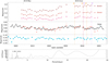 |
Fig. 1. TESS light curve, indicated with a black curve. The flare-like events are colored in blue. The ground-based IJHK-band measurements are shown with colored dots and were shifted along the y-axis by the values indicated in the corresponding labels in the figure. The nightly averaged ASAS-SN g-band observations obtained during the TESS observing period are plotted with blue points. The vertical dashed orange and purple lines show the epochs when the ESPRESSO (E) and FEROS (F) spectra were taken, respectively. The long tickmarks at the top of the figure indicate the beginning of each month. Bottom panel: Lomb-Scargle periodogram obtained using the TESS data. |
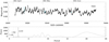 |
Fig. 2. TESS light curve, obtained in 2021, indicated with a black curve. The flare-like events are colored in blue. The long tickmarks at the top of the figure indicate the beginning of each month. Bottom panel: Lomb-Scargle periodogram obtained from the 2021 TESS data. |
The ASAS-SN data taken between 2014 and 2020 have a sparser time coverage than TESS, but are useful to learn about the long-term behavior of CR Cha. We calculated the Lomb-Scargle periodogram for all the available ASAS-SN data taken between 2014 and 2020 (Fig. 3). Since the Lomb-Scargle algorithm suited exploration of the Fourier-spectrum also in the case of unevenly sampled data like ours well, this method is able to reveal the existing periods in the ASAS-SN dataset as well. V-band observations are available between 2014 and 2018, and g-band observations are accessible between 2017 and 2020. The most significant peaks of the periodograms are at P = 2.327 ± 0.0014 in the V band and P = 2.326 ± 0.0019 days in the g band. These periods agree with the stellar rotational period found in the TESS light curves. Moreover, we found significant periods of about one day in the V and g bands, which appear to be due to the fact that the observations were taken with a nightly cadence. An additional 1.754-day period appears to be present in the ASAS-SN data. The TESS data from 2019 do not show signs of a period around 1.7 days, whereas an indication of this periodicity is present in the 2021 observations with TESS. We thus examined whether shorter sections of the ASAS-SN data indicate its presence. We found that during the 2019 TESS observing period, the ASAS-SN data do not show any period around 1.7 days either. However, randomly selected 56-day-long slices of the ASAS-SN light curves show a period around 1.7 days with varying intensity. The origin of this periodic signal is unclear and is surely very variable with time.
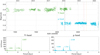 |
Fig. 3. ASAS-SN V- and g-band light curves are shown in the top panel along with epochs when the HARPS (dashed gray lines), the ESPRESSO (dashed orange lines) and the FEROS (dashed purple lines) were taken. The black dots indicate the median brightness for each group of data. Bottom left panel: Lomb-Scargle periodogram for the V-band data, and right panel: Lomb-Scargle periodogram for the g-band data. |
The long-term behavior of the V-band light curve indicates a general, slow brightening of the system by ∼0.05 mag over about four years. This effect is not observed in the g-band light curve, either because the effect is no longer present after 2018, or because the bluer wavelength coverage of the g-band filter weakens the effect.
Similarly to the ASAS-SN data, the available ASAS-3 V-band photometric data, obtained between 2001 and 2009, are useful for studying the long-term trends in CR Cha. These data are shown in the top panel of Fig. 4. We computed the Lomb-Scargle periodogram for the ASAS-3 observations, which we show in the bottom panel of Fig. 4. The data show a well-defined period at P = 2.327 days, which is consistent with the stellar rotation period, and we interpret this signal as rotational modulation due to spots. This period agrees with the previous results and with the other datasets shown here. The 2.3-day period is present in the system for decades, and the most recent high-resolution data also confirm its presence. In the long term, the data reveal an increasing trend in the brightness by ∼0.2 mag over 8 years, which is in line with the brightening observed in the ASAS-SN data. However, no sudden, extreme brightening or dimming was detected, which indicates the stable behavior of the system.
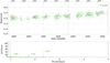 |
Fig. 4. ASAS-3 light curve with the phases when the AAT spectra were taken (top; vertical dashed lines), and the black dots show the median brightness for each group of data. Bottom panel: Lomb-Scarge periodogram for the whole ASAS-3 dataset. |
As the TESS light curve reveals more stochastic variations due to its more frequent timescales sampling, and because the ASAS-SN and ASAS-3 data have longer time coverage, we adopted the P = 2.327-day period as the stellar rotation period found in the ASAS-SN and ASAS-3 data for our target. We used this period to construct the phase-folded light curves (Fig. 5). Before creating the phase-folded light curve for the ASAS-3 data, we subtracted the linear brightening trend and shifted it back to the median brightness level. In addition, we also removed the long-term oscillating trend from the TESS light curve, and shifted it back to the median brightness level. We fit a sine curve to all the different datasets. The datasets are indicated with orange curves in Fig. 5. The TESS light curve (top panel of Fig. 5) reveals a trend that can be better fit with the sum of two sine curves, indicating that multiple spots contribute to the modulation. The peak-to-peak amplitude of the fitted curves show the rotational modulation with different amplitudes in the different bands ranging from ∼0.009 mag in the TESS observations to ∼0.09 mag in the ASAS-3 measurements.
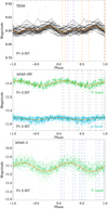 |
Fig. 5. Phase-folded light curves of CR Cha. Vertical dashed lines indicate the epochs of the spectroscopic observations. Top panel: TESS measurements with the ESPRESSO (orange lines) and FEROS (purple lines) epochs, middle panel: ASAS-SN observations with the HARPS epochs (gray lines), and bottom panel: ASAS-3 data with the AAT epochs (dark blue lines). The orange curve shows the fitted sine curves to each data set. |
3.2. Color variations
The IC, J, H, K-band SMARTS observations were obtained simultaneously with the TESS observation (Fig. 1) in the 2019 observing period. For most nights, the ground-based IC-band magnitudes reproduce the space-based broadband optical TESS photometry well. The near-infrared J, H, K-band light curves also follow the variability seen in the TESS observations in the first 20 days, although with smaller amplitude. In contrast, in the second half of the TESS observing window, the near-infrared light curves show a brightening trend of 0.1−0.2 mag, whereas the TESS magnitudes remain constant to within 0.03 mag. Because the time coverage of the data is limited, we did not attempt to perform a periodogram analysis on the ground-based data.
In Fig. 6 we show the color-magnitude and the color–color diagrams obtained from our IC, J, H, K-band measurements. The color-magnitude diagrams indicates that the source becomes redder as it becomes brighter (negative slope). We indicate the more recent data with lighter colors in the color-magnitude diagrams, and they suggest that the system was brightening at near-infrared wavelengths during the last days of the 2019 observing period.
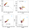 |
Fig. 6. Color-magnitude and color–color diagrams based on SMARTS photometry taken in 2019. The more recent measurements are indicated with lighter colors. The arrow shows a change in extinction of AV = 1 mag. The blue triangles show the (rescaled) models by Carpenter et al. (2001). The color changes for different sizes of the disk inner radius from 1 to 2 and to 4 R⊙. |
The trajectories in the color-magnitude diagrams can help distinguish different possible physical mechanisms that might cause the variability. These physical mechanisms include rotating starspots on the stellar surface, variable accretion, or extinction caused by the circumstellar matter. We indicate the effect of extinction change corresponding to AV = 1 mag in Fig. 6 with an arrow, which highlights that the data are distributed orthogonal to the reddening vector. In addition, the presence of starspots would also result in a positive slope (redder as it becomes fainter) in the color-magnitude diagrams (Carpenter et al. 2001). Therefore, starspots and extinction cannot explain all of the variability characteristics we observed, which suggests the presence of an additional mechanism that affects the emission at longer wavelengths more than at shorter wavelengths. These color variations are discussed in Sect. 4.3. We explored the [g–TESS] versus TESS color-magnitude diagram, the analysis of which resulted in a nearly colorless variation. We also examined whether shorter-term color variations associated with rotation period appear in the color-magnitude diagrams, but we found no significant trends.
3.3. Spectroscopy
In order to display the phase coverage of the spectroscopic observations, we indicate in Fig. 5 with vertical dashed lines the phases in which the spectra were taken that we used in this work. The middle panel of the figure shows that the HARPS data from 2018 cover the whole phase-space. On the other hand, the AAT observations from 2006 do not cover the dimmest phase (bottom panel), and the ESPRESSO and FEROS measurements from 2019 are more sparse in the phase coverage (top panel). Even though two ESPRESSO observations were taken outside of the TESS observing period, we overplot them in the top panel in order to display the phase coverage of all observations.
The shape of the emission line profiles present in the spectra of CR Cha changes throughout the observing seasons on yearly, monthly, and daily timescales. The strongest emission line in all spectra is the Hα line. In addition, we detected the Hβ and the [O I] 630 nm lines in weaker emission. The [O I] 557 nm emission line present in the HARPS and AAT spectra is not astronomical, but due to emission in our atmosphere. This line was removed from the ESPRESSO and the FEROS spectra during the data reduction process. In addition to the emission lines, we detected the Na I doublet and the Li I 670.8 nm absorption lines in all spectra. The Ca II infrared triplet region (CaIRT) is covered only by the FEROS spectra. Because one line of the triplet is located between two orders, only two CaIRT lines were detected, and they appear in weak absorption. In addition, the Ca II H and K lines appear in emission in the ESPRESSO and FEROS spectra, but they are not covered by the AAT observations. The Ca II K line was detected in the HARPS spectra as well, but the noise level is too high to identify the Ca II H line. In the following, we analyze the variability of the two permitted emission lines detected in the spectra and of the veiling of the photospheric lines.
3.3.1. Analysis of the Hα line
The Hα line profile shows both short-term and long-term variability. The mean Hα line profiles for each observing season, indicated with thick black lines in Fig. 7, show that the general Hα line profile has changed remarkably on yearly timescales.
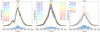 |
Fig. 7. Hα line profiles for all three observing seasons. The mean profiles are indicated by a thick black curve, and the variance profile is shown with blue shaded area. The numbers indicate the JD of observations with the corresponding color. |
All Hα line profiles show a strong central component, but the intensity of this component varies over time. The largest change in the amplitude, including the weakest peaks, appears during the 2019 observing season. However, it should be noted that this observing season is more sparsely sampled, but covers a longer period than the earlier seasons: the sampling probes the monthly timescales. In addition to the amplitude variations, the Hα line exhibits morphological variations. A red bump appears at about 100 km s−1 on the night with the strongest emission, moreover, the entire blue wing becomes relatively strong during one of our observations. In contrast, the 2006 data display different line profiles with respect to the more recent datasets. The central peak reaches a maximum among our spectra, but also varies by a factor of 1.5 in peak intensity. A strong blueshifted absorption feature is present around −100 km s−1, and this line profile shape is preserved during the entire 2006 observing period with varying amplitudes. The 2018 data show very stable line profiles during the entire HARPS observing period with a small amplitude variation. A small blue absorption appears here as well, but the profiles are more symmetric than in 2019.
In order to examine the temporal variance of the line profiles in each velocity bin, we calculated the variance profile as described in Johns & Basri (1995). We show the variance profiles in Fig. 7 as the blue shaded areas. The variance profiles indicate the strongest variability of the lines at the central peak for all three observing periods, with the largest amplitude variations in 2019. This is likely caused by the varying accretion onto the star. The 2018 data show only small amplitude changes with little variations of the amplitude with velocity. In contrast, the 2006 observations indicate variability at the dip around −100 km s−1 as well as changes in the amplitude of the central peak, which might indicate a varying wind component. Finally, the 2019 data show strong variations both in the central peak and at +100 and −100 km s−1. While the latter could be again ascribed to a varying wind, the former is possibly the result of varying accretion geometry.
We show the Hα line profiles ordered by phase for all observations in Fig. 8 along with the median profile indicated in black. The 2006 observations in the top panel show that the blueshifted absorption around −100 km s−1 becomes more pronounced from phase 0 to 0.3, then the strength of the component approaches the level of the median profile toward the photometric minimum. As the light curve comes out of a minimum, the absorption again becomes more pronounced. The redshifted excess emission compared to the median profile around 150 km s−1 weakens as the phase progresses, and it is weakest right before the minimum. After the photometric minimum, this component strengthens again.
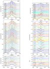 |
Fig. 8. Hα spectra ordered by rotation phase (left), and the Hβ lines ordered by rotation phase (right) for each observing season. Top panels: AAT, middle panels: HARPS, and bottom panels: ESPRESSO and FEROS measurements. The phases with rotational number are indicated on the left side of each line. The thick black lines indicate the mean line profile for each observing season. |
We show the Hα line profiles ordered by phase for the 2018 observations in the middle panel of Fig. 8. In this case, the blueshifted bump at −150 km s−1 becomes stronger from phase 0 to phase 0.2. Toward the photometric minimum, this component becomes weaker than the median value, but it becomes stronger again closest to the minimum. As the light curve leaves the minimum, this component weakens again. At the same time, the central peak weakens from phase 0 to phase 0.4, but it also becomes stronger closest to the minimum, and weakens again as the light curve leaves the minimum.
The bottom panel of Fig. 8 shows the 2019 ESPRESSO and FEROS observations ordered by phase. Because these observations cover a longer time span, they are less sensitive to the variability on short timescales, but they can reveal the variability on monthly timescales. This shows that the amplitude of central component of the Hα line is highly variable during our observing period, which suggests changing accretion onto the central star.
The observed emission lines consist of multiple components and display variability on various timescales. These components might originate from different physical processes. In order to examine the relation between the variations of these components, we calculated correlation matrices (Johns & Basri 1995). We divided each emission line into small velocity intervals and calculated the correlation coefficient (r) between every pair of velocity bins as follows:
where x and y contain the intensity values of each epoch for a chosen velocity bin. Calculating the correlation coefficient between every pair of velocity bin results in a correlation matrix.
The autocorrelation matrices for the Hα lines are shown in Fig. 9. The 2006 observations show correlation in the blue wing of the Hα line, between around −150 and −250 km s−1. There is also an anticorrelation between about −80 and −250 km s−1, and −80 and −150 km s−1. The pattern is slightly different for the 2018 observations: anticorrelation appears between the red and the blue parts of the line, at ∼50 and −120 km s−1. The ESPRESSO and FEROS observations resulted in very different autocorrelation matrices. This probably results from the larger temporal gap between the individual observation.
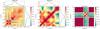 |
Fig. 9. Correlation matrices for the Hα lines. The positive values (darker red) indicate a correlation, the negative values (darker blue) show an anticorrelation, and the values around zero (yellow) indicate no correlation. Left: 2006 (AAT), middle: 2018 (HARPS), right: 2019 (ESPRESSO and FEROS). |
In order to examine whether the photometry and the spectroscopy are linked in a way that lines vary with the same period as the photometric brightness, we applied a Lomb-Scargle periodogram analysis in each velocity bin for the Hα and the Hβ lines. The resulting 2D periodograms for the 2006 and the 2018 observing seasons are plotted in Fig. 10. We drew contours around the regions corresponding to the 85% and 95% confidence levels.
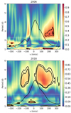 |
Fig. 10. Two-dimensional periodogram for the Hα lines. The color bar represents the periodogram power varying from zero (blue) to maximum power (red). The inner contours correspond to the 95% confidence level, and the outer contours correspond to the 85% confidence level. The stellar rotational period is marked by the horizontal dashed white line. |
During the 2006 observing season, the red wing of the Hα line and the blueshifted absorption component (∼100 km s−1) showed significant periodic behavior with a period of ∼1.1 days, about half of the stellar rotation period. As the data cover 4.24 days, which is less than the twice the rotational period, we might not be sensitive to variability on timescales of the rotation period. However, a ∼2- to 3-day period was found in the redshifted wing of the Hα line with a 85% confidence level. In contrast, the 2018 HARPS observations reveal a somewhat longer periodicity (∼3−5 days) in the redshifted side between 0 and 250 km s−1 and on the blueshifted side between −100 and −200 km s−1, and do not seem to be modulated by the rotational period.
3.3.2. Analysis of the Hβ line
The profile of the Hβ line also displays variability throughout the years, but during a given observing period, it shows variability with small amplitude. We calculated the normalized variance profiles as described above, and indicate them as the blue shaded area in Fig. 11.
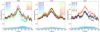 |
Fig. 11. Hβ line profiles for all three observing seasons. The mean profiles are indicated by a thick black curve, and the variance profile is shown as the blue shaded area. |
There are several photospheric absorption lines in the Hβ region, which are superposed on the Hβ emission. In order to eliminate the effects of the absorption lines, we subtracted the rotationally broadened spectrum of ϵ Eri, which has the same spectral type as CR Cha, from the observed spectra. This process resulted in more defined peaks. The results show (Fig. 11) that most of the variability comes from the amplitude changes of the line during all observing seasons. On the other hand, the strength of the mean line profile slightly changes throughout the years. Overall, the lines vary not as strongly as the Hα line. We present the Hβ line profiles ordered by phase in Fig. 8. The results show a similar pattern in the amplitude variations as the Hα line, but no significant morphological variations were found.
The 2D periodograms for the Hβ line are shown in Fig. 12. The 2006 measurements reveal a period of about the rotation period in the red wing of the line, but the 2018 data only show a period of ∼3−4 days, similarly to Hα, but with a smaller extent in terms of velocity.
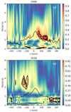 |
Fig. 12. Two-dimensional periodogram for the Hβ lines. The color bar represents the periodogram power, and the inner contours correspond to the confidence levels (as in Fig. 10). |
3.3.3. Veiling measurements
The photospheric spectrum of classical T Tauri stars is often veiled by additional continuum emission. The veiling continuum is attributed to the shock-heated gas, which results in a hot spot on the stellar surface below the accretion stream. The veiling of a star can be determined by measuring the equivalent widths of photospheric lines,
where Weq is the measured equivalent width,  is the reference equivalent width, and V is the veiling.
Instead of using only a single absorption line, we constructed an average absorption line profile using the least-squares deconvolution (LSD) method (Donati & Collier Cameron 1997). We used the unpolarized LSD profiles to calculate the veiling, but because veiling is wavelength dependent, we recalculated the LSD profiles for a smaller region of the spectrum between 530 and 700 nm. As ϵ Eri is a nonaccreting star with the same spectral type as CR Cha, we used the rotationally broadened spectrum of ϵ Eri as a reference spectrum in order to calculate the absolute veiling of CR Cha. CR Cha shows moderate veiling of ∼0.2 with small variations. As veiling is often considered a measure of the accretion rate, the small veiling variations indicate a modest change in the accretion rate by a factor of ∼3.
We also examined whether the veiling, which was obtained from the absorption lines, varies in phase with the rotation period. Figure 13 shows that the majority of the veiling values is almost constant, and the values are only slightly modulated by the rotational period. However, we note that our results show three additional outlying data points in terms of the veiling at phases 0.33 and 0.76, which are beyond the range of Fig. 13.
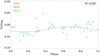 |
Fig. 13. Veiling variations during the three observing seasons as a function of orbital phase, using the P = 2.327-day period obtained from our period analysis of the light curves. |
4. Discussion
CR Cha shows small-amplitude but significant photometric variability on timescales from hours to years, with a peak-to-peak amplitude ranging from ∼0.05 mag in the optical TESS observations to ∼0.15 mag in the K-band data. Periodic behavior was found in the two new TESS observations from 2019 to 2021 and archive ASAS-SN (2014–2020) and ASAS-3 (2000–2010) catalogs. This confirmed that the ∼2.3-day periodicity is present in the system for decades. This periodicity can be attributed to stellar rotation caused by spots on the stellar surface. The brightness variations can be modeled with simple spot models, but the available colors and the uncertainty on each value do not allow us to distinguish between cold (T ∼ 4350 K) and hot (T ∼ 5300 K) spots. It is likely that both exist on the surface of this star, which is known to host a complex magnetic field (Hussain et al. 2009). In addition,
the ASAS-3 and the ASAS-SN V-band observations indicate a general, slow brightening of the system: the ASAS-3 data show ∼0.2 mag brightening during about eight years of observations, and the ASAS-SN V-band light curve indicates a brightening of ∼0.05 mag over about four years. The origin of this brightening is unclear, but it changes in the average spot coverage as spots that slowly evolve over time might contribute to the observed behavior effect. On the other hand, the TESS data with their much higher photometric accuracy reveal a more stochastic behavior with peak-to-peak amplitude of ∼0.05 mag, probably due to accretion variability, and a few flares. The shapes of the multifilter J-, H-, and K-band light curves are similar to those of the TESS light curve, but the amplitude of the variability is different. The J-band data have the smallest amplitude of ∼0.09 mag, and the amplitude increases toward the K band, which has a peak-to-peak amplitude of ∼0.17 mag. While the TESS data probe the variability on the shortest timescales, ground-based photometry reveals a trend beyond the rotational modulation.
The most striking variable features in the spectra are the highly variable Balmer emission lines. The mean Hα line profiles show strong variations in both intensity and line profiles on a yearly timescale. This suggests that different physical mechanisms contribute to the observed variability. In this section we discuss how we interpret these spectroscopic and photometric variations.
4.1. Line morphology variations
We discuss here the variability of the emission line profiles during the three observing periods. The observed shifts in the variability period on decadal timescales might originate from the formation of multiple hot spots on the stellar surface at different times: one dominant hot spot would cause modulation at the stellar rotation period, while multiple hot spots at different latitudes would result in different variability periods. Multiple hot spots are expected on CR Cha, as the star hosts a complex magnetic field (Hussain et al. 2009). As the phase coverage of the 2019 observations is poorer than that of the previous epochs, we cannot check if there is any periodicity.
In comparison with studies focused on other T Tauri systems, the period analysis of the Hα lines for this target often do not exhibit a single and highly significant peak. As the Hα line is expected to form not only at the accretion spot, but also in the accretion funnel and in the stellar winds, the variability of this line is also influenced by the variations of the circumstellar environment. However, the rotation period might appear with varying strengths in the periodograms. It is instructive to compare our findings with similar analyses of individual targets. In the LkCa 15 system, the strength of the emission at the line center is modulated by stellar rotation, and this effect is clearly displayed in the periodogram (Alencar et al. 2018). On the other hand, the inverse P Cygni profile of the Hα line of the HQ Tau system displays modulation on the timescale of the stellar rotation not only in the line center, but all the way to the red wing (Pouilly et al. 2020). Another interesting system to mention is V2129 Oph. When analyzing this target, Sousa et al. (2021) compared their results with the periodograms for the same system as was analyzed by Alencar et al. (2012), and they found some differences on timescales of a decade, similarly to our results. Sousa et al. (2021) discussed a few possible explanations for the observed phenomena, such as variations in the magnetic field strength, which would result in variations in the magnetospheric truncation radius, or latitudinal differential rotation, or a more complex magnetic structure with two major funnel flows originating at different radii in the inner disk. However, in the case of V2129 Oph, a periodicity longer than the stellar rotation period is present at the line center for a time of almost a decade. The likely cause of the periodicity is a structure that is present beyond the corotation radius that is stable for almost a decade. In the case of CR Cha, the rotation period has been stable for decades, but the line profiles (and the photometry as well) also vary with longer periods, likely because of variations in the circumstellar environment.
The overall Hα line profile variations show different characteristics during the three observing seasons, indicating the significance of different variable physical mechanisms on a yearly timescale. The 2018 observations show the least amount of variability, mostly showing modulations presumably due to changes in the accretion rate. The 2006 observations reveal a slightly different line profile with an additional blueshifted absorption component, which is usually associated with ejection processes, such as wind. In addition, the amplitude variations of the central peak are larger than those during the HARPS observations in 2018, which suggests a stronger change in the accretion rate. The 2019 observations show line profiles similar to those measured in 2018, but based on their variance profile, these data show the largest amount of variability due to the changing accretion, similarly to the 2018 observing season.
The Hβ line profiles do not show as prominent morphological changes as the Hα lines. However, the amplitude of the Hβ lines vary both over the observing seasons and within one set of observations. The 2018 data show the least amount of variability, similarly to the Hα line, indicating very small changes in the accretion rate. The 2019 and 2006 data exhibit a comparable and a larger amount of variability across the whole line, which indicates slightly stronger changes in the accretion rate. We quantify these variations in the next section.
4.2. Timescales of accretion variability
After describing how the observed emission lines vary in morphology with time, we wish to investigate the timescales on which these variations are largest. Our data allow us to explore the timescales from hours to a decade in one particular object. We calculated the equivalent width of the Hα line at each epoch, and because our photometric observations indicate that the brightness of the star barely changes, the equivalent width should be proportional to flux variations. In order to confirm that the variations in equivalent width roughly correspond to variations in accretion rates, we converted the equivalent width values into accretion rates for each observation with the following procedure. First, we calculated the Hα line luminosity using the continuum flux value around the Hα line measured on the flux-calibrated X-shooter spectra of this target in 2010 (Manara et al. 2016). As the mean brightness of the system did not change significantly between 2010 and 2019 (see Figs. 3 and 4), we used the same continuum flux value for both the 2018 and the 2019 observations, whereas we accounted for the ∼0.1 mag dimmer state during the 2006 by decreasing the continuum flux by the corresponding flux ratio. The line luminosity was then converted into accretion rate using the empirical relation from Alcalá et al. (2017). Finally, we computed Ṁacc with the classical relation (Hartmann et al. 2016). The values of Ṁacc at the time of our observations are shown in Fig. 14, and fall between ∼2−5 × 10⁻⁹ M⊙ yr−1, in line with previous results (e.g., Manara et al. 2016, 2019).
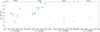 |
Fig. 14. Mass accretion rates calculated at each observing epoch from the estimated luminosity of the Hα line for CR Cha. |
We then obtained the relative amplitude of the accretion rate variations compared to the mean accretion rate value. In order to cover all the possible timescales from our dataset, every value of the accretion rate was compared with the values obtained from every other spectrum. They are displayed with small blue dots in Fig. 15. We also mark the median amplitude of the variations for the different timescales with larger colored dots, and indicate the 0.25 to the 0.75 percentile of the distribution of the points with black lines. Our results show that the amplitude of the variations increases from hours to several days, and it saturates when in the range between a week to a month, which is not well sampled by our data. This result partially agrees with the conclusions of Costigan et al. (2014). The comparison of this result with the stellar rotation period suggests that the maximum of the variations is on timescales that are longer than the rotation period, whereas Costigan et al. (2014) suggested that the maximum variability is on timescales of about the rotation period. In addition, there is an apparent drop at the timescales of a decade. However, this effect might arise from the fact that our sample on a decadal timescale contains fewer data than on shorter timescales.
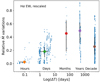 |
Fig. 15. Relative variations in Ṁacc, computed from the estimated luminosity of the Hα line, on timescales from hours to 13 years. |
Studies of large samples of low-mass young stars show that the amplitudes of the variability in the accretion rate range from small fractions to about one order of magnitude, with typical value of ∼0.4 dex (Venuti et al. 2014; Manara et al. 2021). In this context, the accretion rate of CR Cha is smaller than the typical value for young stars with mass > 1 M⊙, but the accretion rate variations of CR Cha reach the typical value presented in Venuti et al. (2014). The typical timescales of accretion variability of classical T Tauri stars has also been explored in previous works in the framework of large surveys. Nguyen et al. (2009) examined the spectra of several low-mass pre-main-sequence stars and found that the amplitude of the variations increases from hours to several days, after which it saturates. Costigan et al. (2012) analyzed the optical spectra of 25 targets in the Chamaeleon I region and derived an upper limit on the dominant timescale of the accretion variability: They suggested that observations on timescales of a few weeks are sufficient to characterize the majority of the accretion-related variations in typical young stars over a period of about one year. Costigan et al. (2014) studied 15 T Tauri and Herbig Ae stars over a wide range of timescales and found that the majority of the variations occurs as gradual changes in the Hα emission and that the period of days is the dominant timescale of these variations. Our data confirm that accretion variability has a maximum of intensity on timescales of weeks to months.
4.3. Explanation of the color variations
As discussed in Sect. 3.2, the data we have obtained allow us to study the variations in the near-infrared colors for CR Cha in 2019. We compare these variations with the models developed by Carpenter et al. (2001).
Carpenter et al. (2001) examined the near-infrared color variations of young stars and described three physical models as the possible origin of the observed color changes. In the first of their models, the light variations are caused by starspots, which modulate the brightness of a star as stellar rotation alters the fractional spot coverage. This model resulted in either nearly colorless fluctuations or in a positive slope on the color-magnitude diagram (i.e., the object becomes bluer as it becomes brighter), depending on the fractional spot coverage and spot temperature. This is not observed for CR Cha. The extinction model attributes the observed color changes to extinction, which results from inhomogeneities in either the inner circumstellar environment or in the molecular cloud that move across the line of sight. The extinction vectors can be calculated from the interstellar reddening law, and they also result in a positive slope on the color-magnitude diagram. However, the extinction slope is shallower by 25° than the slopes expected from hot spots. Again, this is not what is observed for our target.
The third model that Carpenter et al. (2001) considered is an accretion disk model, which takes the emission from a circumstellar disk as a source of near-infrared variability into account. The near-infrared variability may originate either from changes in the mass accretion rate or from changes in the inner disk structure that alter the amount of absorbed and reprocessed stellar radiation. Variations in the accretion rate or in the structure of the inner disk result in a negative slope in the near-infrared color-magnitude diagram. This negative slope (target becomes redder as it becomes brighter) in the color-magnitude diagrams we observe in CR Cha (Fig. 6) is peculiar and is typically observed in a small fraction of targets (∼1%, Carpenter et al. 2001). This behavior suggests that the color variations are not due to changing extinction or to the presence of stellar spots, but are more consistent with the accretion disk model described by Carpenter et al. (2001).
Based on our available data, we can attempt to test the hypothesis that the variations in Ṁacc are the cause of the color variability. In order to test this hypothesis, we compared the equivalent widths of the Hα lines in the 2019 observing epoch (Table 1) with the data points on the color-magnitude diagrams that were taken on the same nights (indicated in green in Fig. 6). Unfortunately, as these data points only cover a small range in the diagram, it is difficult to recognize any pattern. However, a rough comparison is possible. The disk model in Carpenter et al. (2001) indicates that the expected photometric variations can be a few tenths of a magnitude for accretion rates changing from Ṁ ∼ 3 × 10⁻⁹ M⊙ yr−1 to Ṁ = 10−7 M⊙ yr−1. The comparison between these models and our photometric data suggests that, if the color variations are only due to accretion rate variations, the variability of the accretion rate during our observations were smaller than a factor of ∼5. This is in line with equivalent width variations, which indicate that the accretion rate varies by a factor of ∼3. Thus, the possibility that the color variations are due to an accretion rate variation is compatible with our data.
Equivalent widths of the Hα lines for the 2019 campaign.
On the other hand, variations in the size of the disk inner hole, or variations in the thickness of the inner edge of a warped disk, may also result in changes in the reprocessed radiation (e.g., Carpenter et al. 2001). The models of Carpenter et al. (2001) suggest a variation of a few tenths of a magnitude in the near-infrared bands when the size of the disk inner hole changes between 1 R⊙ and 4 R⊙. CR Cha shows variation smaller than one-tenth of a magnitude in Fig. 6, indicating a smaller change in the size of the inner hole. We indicate in Fig. 6 the model values of the color and the magnitude changes from Carpenter et al. (2001) with respect to the bluest datapoint of our observations on each panel. Our data line up with two of the open triangles, which corresponds to a change in the sizes of the inner hole from 4 to 2 R⊙ in the case of a mass-accretion rate of Ṁ ∼ 3 × 10⁻⁹ M⊙ yr−1, which is in line with the measured value for CR Cha. Therefore, variations in the structure of the inner disk are also in line with the observations.
Roquette et al. (2020) carried out an investigation of the near-infrared color variations of a large sample of young stars using J-, H-, and K-band observations. They calculated the trajectories in the color space and measured slopes for stars describing linear trajectories. They found that 115 systems of the 144 measured  slopes had negative slopes. On the other hand, only 3 systems of the 196 measured
  slopes had negative slopes. This might imply that the amplitudes of the variability that are due to variable accretion rate and changes in the inner disk are more significant for J magnitude and J − H color than for K magnitude and H − K color. However, the flux in the J band is mainly dominated by stellar flux, whereas the amount of light that is re-emitted by the disk in the near-infrared is larger for longer wavelengths. All in all, Roquette et al. (2020) still found 1.7 times more stars with variability caused by extinction or a spot than caused by changes in the inner disk or accretion, which places CR Cha in the class of the rarer systems.
Unfortunately, we cannot measure the size of the inner disk hole with our data. However, the circularly polarized spectra from our 2006 AAT and 2018 HARPS observations allow us to derive the expected magnetic field truncation radius (Rtr). Hussain et al. (2009) showed that CR Cha hosts a complex magnetic field that also includes dipole and octuple magnetic field components. As the dipole component is expected to truncate the disk while the octupole dominates on a smaller scale and at the surface of the star (Gregory et al. 2008), we determined the magnetospheric truncation radius using the dipole component. Assuming a dipole field configuration, the magnetic field truncation radius can be calculated using the following relation (Bouvier et al. 2007):
We caution that this relation to derive the truncation radius may not be applicable to stars hosting complex multipolar fields. With this caveat, we can calculate Rtr for CR Cha. According to Hussain et al. (2009), the dipole component of the large-scale magnetic field is ∼100 G; this results in Rtr = 2.9 R⋆, which is equivalent to 7.3 R⊙, assuming R⋆ = 2.5 R⊙ (Hussain et al. 2009). Figure 6, depicting the 2019 data, indicates that the change in the size of the inner disk hole is from 4 R⊙ to 1 R⊙. Ignoring variations in Ṁacc, on which Rtr depends only little, this variation would imply a variation in B⋆ of 24 G. Unfortunately, our data cannot test this variations. Future studies should aim to cover several rotational periods with spectropolarimetric data and near-infrared photometry to test whether variations in the magnetic field strength, and thus in the truncation radius, are compatible with the observed color variations. For now, we can only conclude that the variations in the near-infrared colors are compatible with the observed variations in Ṁacc, but we cannot exclude that variations in the inner disk structure also contribute to these color variations.
5. Conclusions
We presented a spectroscopic and photometric study of the classical T Tauri star CR Cha. We examined several datasets from three different observing seasons in 2006, 2018, and 2019. Based on the analysis of the photometric data, we found that a 2.326-day period is present in the dataset, which agrees with the stellar rotation period. This indicates that the photometric variations are modulated by the stellar rotation period due to the presence of stellar spots. In addition, the TESS light curves revealed a few flare-like events thanks to its high temporal resolution. By comparing the color changes of the I-, J-, H-, and K-band observations with the models of Carpenter et al. (2001), we found that the color variations are due to changes in the inner disk properties. These can be due to variations in the mass accretion rates compatible with those we observe, or with changes in the inner hole size of the circumstellar disk.
The presence of the hydrogen Balmer lines allowed us to examine the accretion process in more detail. The Hα line shows the largest variability in shape in 2019, whereas it showed only small-amplitude variations in 2018. The comparison between the three observing seasons indicates significant morphological changes, but the variations in central peak strengths due to changes in the accretion were the most significant differences in all observing seasons.
Our extensive dataset allowed us to examine the variability on timescales from minutes to decades. The photometric data can be interpreted as variations on timescales of ∼2.3 days due to stellar rotation. On a decadal timescale, we found a slight brightening trend, and on the shortest timescales of minutes to hours, flare-like (∼0.02 mag) events also cause short brightenings.
The Hα line amplitude, thus accretion rate changes, show fluctuations on a wide range of timescales. The amplitude of the variability increases from minutes to several days, and it saturates when it reaches the timescale of weeks to months. Our results suggest that about a week is the dominant timescale of accretion variability for this target. This is in line with previous works and suggest that, apart from secular variability, any measurement of accretion is likely to vary by ∼0.4 dex on a timescale of weeks to months.
Future works covering various timescales of variability with spectroscopy should aim at covering the phase of the periodicity of the target at all observing seasons, which would provide the possibility of verifying whether variations in accretion are due to variations in the magnetic field topology. CR Cha belongs to the rare class of targets that becomes bluer when fainter at infrared wavelengths. This phenomenon should be investigated with surveys, in order to verify whether the size of the inner disk varies with time, as suggested by the models. In the brightest of these systems, it would be important to assess whether this behavior is predominantly associated with a particular type of stellar magnetic field (e.g., complex, variable multipolar fields, or more stable simple axisymmetric fields).
Acknowledgments
G.Zs. has received support from the ESO Studentship Program Europe. This project has received funding from the European Research Council (ERC) under the European Union’s Horizon 2020 research and innovation program under grant agreement No. 716155 (SACCRED). This project has received funding from the European Union’s Horizon 2020 research and innovation program under the Marie Sklodowska-Curie grant agreement No. 823823 (DUSTBUSTERS). This research received financial support from the project PRIN-INAF 2019. This work was partly supported by the Deutsche Forschungs-Gemeinschaft (DFG, German Research Foundation) – Ref no. FOR 2634/1 TE 1024/1-1. “Spectroscopically Tracing the Disk Dispersal Evolution”. The research leading to these results has received funding from the LP2018-7 Lendület grants of the Hungarian Academy of Sciences. G.Zs. is supported by the ÚNKP20-3 New National Excellence Program of the Ministry for Innovation and Technology from the source of the National Research, Development and Innovation Fund. This work has received financial support of the Hungarian National Research, Development and Innovation Office NKFIH Grant K-138962. We thank K. Vida for the service in the spot modeling.
References
- Alcalá, J. M., Natta, A., Manara, C. F., et al. 2014, A&A, 561, A2 [NASA ADS] [CrossRef] [EDP Sciences] [Google Scholar]
- Alcalá, J. M., Manara, C. F., Natta, A., et al. 2017, A&A, 600, A20 [NASA ADS] [CrossRef] [EDP Sciences] [Google Scholar]
- Alencar, S. H. P., Bouvier, J., Walter, F. M., et al. 2012, A&A, 541, A116 [NASA ADS] [CrossRef] [EDP Sciences] [Google Scholar]
- Alencar, S. H. P., Bouvier, J., Donati, J.-F., et al. 2018, A&A, 620, A195 [NASA ADS] [CrossRef] [EDP Sciences] [Google Scholar]
- Bailer-Jones, C. A. L., Rybizki, J., Fouesneau, M., et al. 2021, AJ, 161, 147 [NASA ADS] [CrossRef] [Google Scholar]
- Bouvier, J., Bertout, C., Benz, W., et al. 1986, A&A, 165, 110 [NASA ADS] [Google Scholar]
- Bouvier, J., Alencar, S. H. P., Harries, T. J., et al. 2007, in Protostars and Planets V, eds. B. Reipurth, D. Jewitt, & K. Keil, 479 [Google Scholar]
- Brahm, R., Jordán, A., & Espinoza, N. 2017, PASP, 129, 034002 [Google Scholar]
- Calvet, N., & Gullbring, E. 1998, ApJ, 509, 802 [Google Scholar]
- Carpenter, J. M., Hillenbrand, L. A., & Skrutskie, M. F. 2001, AJ, 121, 3160 [NASA ADS] [CrossRef] [Google Scholar]
- Cody, A. M., Stauffer, J., Baglin, A., et al. 2014, AJ, 147, 82 [Google Scholar]
- Costigan, G., Scholz, A., Stelzer, B., et al. 2012, MNRAS, 427, 1344 [Google Scholar]
- Costigan, G., Vink, J. S., Scholz, A., et al. 2014, MNRAS, 440, 3444 [NASA ADS] [CrossRef] [Google Scholar]
- Cutri, R. M., Skrutskie, M. F., van Dyk, S., et al. 2003, VizieR Online Data Catalog: II/246 [Google Scholar]
- D’Antona, F., & Mazzitelli, I. 1994, ApJS, 90, 467 [Google Scholar]
- Donati, J.-F., & Collier Cameron, A. 1997, MNRAS, 291, 1 [Google Scholar]
- Donati, J.-F., Semel, M., Carter, B. D., et al. 1997, MNRAS, 291, 658 [NASA ADS] [CrossRef] [Google Scholar]
- Donati, J.-F., Collier Cameron, A., Hussain, G. A. J., et al. 1999, MNRAS, 302, 437 [NASA ADS] [CrossRef] [Google Scholar]
- Donati, J.-F., Collier Cameron, A., Semel, M., et al. 2003, MNRAS, 345, 1145 [NASA ADS] [CrossRef] [Google Scholar]
- Donati, J.-F., Morin, J., Petit, P., et al. 2008, MNRAS, 390, 545 [NASA ADS] [CrossRef] [Google Scholar]
- Donati, J.-F., Bouvier, J., Walter, F. M., et al. 2011, MNRAS, 412, 2454 [Google Scholar]
- Donati, J.-F., Hébrard, E., Hussain, G., et al. 2014, MNRAS, 444, 3220 [NASA ADS] [CrossRef] [Google Scholar]
- Freudling, W., Romaniello, M., Bramich, D. M., et al. 2013, A&A, 559, A96 [NASA ADS] [CrossRef] [EDP Sciences] [Google Scholar]
- Gaia Collaboration (Brown, A. G. A., et al.) 2018, A&A, 616, A1 [NASA ADS] [CrossRef] [EDP Sciences] [Google Scholar]
- Gregory, S. G., Matt, S. P., Donati, J.-F., et al. 2008, MNRAS, 389, 1839 [NASA ADS] [CrossRef] [Google Scholar]
- Hartmann, L., Herczeg, G., & Calvet, N. 2016, ARA&A, 54, 135 [Google Scholar]
- Hébrard, É. M., Donati, J.-F., Delfosse, X., et al. 2016, MNRAS, 461, 1465 [CrossRef] [Google Scholar]
- Henden, A. A., Levine, S., Terrell, D., et al. 2015, Am. Astron. Soc. Meet. Abstr., 225, 336.16 [NASA ADS] [Google Scholar]
- Herbig, G. H. 1962, Adv. Astron. Astrophys., 1, 47 [Google Scholar]
- Herbst, W., Herbst, D. K., Grossman, E. J., et al. 1994, AJ, 108, 1906 [NASA ADS] [CrossRef] [Google Scholar]
- Hussain, G. A. J., Collier Cameron, A., Jardine, M. M., et al. 2009, MNRAS, 398, 189 [Google Scholar]
- Johns, C. M., & Basri, G. 1995, AJ, 109, 2800 [Google Scholar]
- Jordi, K., Grebel, E. K., & Ammon, K. 2006, A&A, 460, 339 [NASA ADS] [CrossRef] [EDP Sciences] [Google Scholar]
- Kim, S., Takahashi, S., Nomura, H., et al. 2020, ApJ, 888, 72 [Google Scholar]
- Kochanek, C. S., Shappee, B. J., Stanek, K. Z., et al. 2017, PASP, 129, 104502 [Google Scholar]
- Lomb, N. R. 1976, Ap&SS, 39, 447 [Google Scholar]
- Manara, C. F., Beccari, G., Da Rio, N., et al. 2013, A&A, 558, A114 [NASA ADS] [CrossRef] [EDP Sciences] [Google Scholar]
- Manara, C. F., Fedele, D., Herczeg, G. J., et al. 2016, A&A, 585, A136 [NASA ADS] [CrossRef] [EDP Sciences] [Google Scholar]
- Manara, C. F., Mordasini, C., Testi, L., et al. 2019, A&A, 631, L2 [NASA ADS] [CrossRef] [EDP Sciences] [Google Scholar]
- Manara, C. F., Frasca, A., Venuti, L., et al. 2021, A&A, 650, A196 [NASA ADS] [CrossRef] [EDP Sciences] [Google Scholar]
- Muzerolle, J., Calvet, N., & Hartmann, L. 1998, ApJ, 492, 743 [NASA ADS] [CrossRef] [Google Scholar]
- Muzerolle, J., Calvet, N., & Hartmann, L. 2001, ApJ, 550, 944 [Google Scholar]
- Nagy, Z., Szegedi-Elek, E., Ábrahám, P., et al. 2021, MNRAS, 504, 185 [NASA ADS] [CrossRef] [Google Scholar]
- Nguyen, D. C., Scholz, A., van Kerkwijk, M. H., et al. 2009, ApJ, 694, L153 [NASA ADS] [CrossRef] [Google Scholar]
- Pál, A. 2012, MNRAS, 421, 1825 [Google Scholar]
- Pál, A., Szakáts, R., Kiss, C., et al. 2020, ApJS, 247, 26 [CrossRef] [Google Scholar]
- Piskunov, N., Snik, F., Dolgopolov, A., et al. 2011, The Messenger, 143, 7 [NASA ADS] [Google Scholar]
- Plachy, E., Pál, A., Bódi, A., et al. 2021, ApJS, 253, 11 [NASA ADS] [CrossRef] [Google Scholar]
- Pojmanski, G. 2003, Acta Astron., 53, 341 [NASA ADS] [Google Scholar]
- Pouilly, K., Bouvier, J., Alecian, E., et al. 2020, A&A, 642, A99 [NASA ADS] [CrossRef] [EDP Sciences] [Google Scholar]
- Reiners, A., & Basri, G. 2009, A&A, 496, 787 [NASA ADS] [CrossRef] [EDP Sciences] [Google Scholar]
- Ricker, G. R., Winn, J. N., Vanderspek, R., et al. 2015, J. Astron. Telesc. Instrum. Syst., 1, 014003 [Google Scholar]
- Robinson, C. E., Espaillat, C. C., & Owen, J. E. 2021, ApJ, 908, 16 [NASA ADS] [CrossRef] [Google Scholar]
- Roquette, J., Alencar, S. H. P., Bouvier, J., et al. 2020, A&A, 640, A128 [NASA ADS] [CrossRef] [EDP Sciences] [Google Scholar]
- Scargle, J. D. 1982, ApJ, 263, 835 [Google Scholar]
- Shappee, B. J., Prieto, J. L., Grupe, D., et al. 2014, ApJ, 788, 48 [Google Scholar]
- Siess, L., Dufour, E., & Forestini, M. 2000, A&A, 358, 593 [Google Scholar]
- Sousa, A. P., Bouvier, J., Alencar, S. H. P., et al. 2021, A&A, 649, A68 [NASA ADS] [CrossRef] [EDP Sciences] [Google Scholar]
- Venuti, L., Bouvier, J., Flaccomio, E., et al. 2014, A&A, 570, A82 [NASA ADS] [CrossRef] [EDP Sciences] [Google Scholar]
All Tables
All Figures
|
Fig. 1. TESS light curve, indicated with a black curve. The flare-like events are colored in blue. The ground-based IJHK-band measurements are shown with colored dots and were shifted along the y-axis by the values indicated in the corresponding labels in the figure. The nightly averaged ASAS-SN g-band observations obtained during the TESS observing period are plotted with blue points. The vertical dashed orange and purple lines show the epochs when the ESPRESSO (E) and FEROS (F) spectra were taken, respectively. The long tickmarks at the top of the figure indicate the beginning of each month. Bottom panel: Lomb-Scargle periodogram obtained using the TESS data. |
| In the text | |
|
Fig. 2. TESS light curve, obtained in 2021, indicated with a black curve. The flare-like events are colored in blue. The long tickmarks at the top of the figure indicate the beginning of each month. Bottom panel: Lomb-Scargle periodogram obtained from the 2021 TESS data. |
| In the text | |
|
Fig. 3. ASAS-SN V- and g-band light curves are shown in the top panel along with epochs when the HARPS (dashed gray lines), the ESPRESSO (dashed orange lines) and the FEROS (dashed purple lines) were taken. The black dots indicate the median brightness for each group of data. Bottom left panel: Lomb-Scargle periodogram for the V-band data, and right panel: Lomb-Scargle periodogram for the g-band data. |
| In the text | |
|
Fig. 4. ASAS-3 light curve with the phases when the AAT spectra were taken (top; vertical dashed lines), and the black dots show the median brightness for each group of data. Bottom panel: Lomb-Scarge periodogram for the whole ASAS-3 dataset. |
| In the text | |
|
Fig. 5. Phase-folded light curves of CR Cha. Vertical dashed lines indicate the epochs of the spectroscopic observations. Top panel: TESS measurements with the ESPRESSO (orange lines) and FEROS (purple lines) epochs, middle panel: ASAS-SN observations with the HARPS epochs (gray lines), and bottom panel: ASAS-3 data with the AAT epochs (dark blue lines). The orange curve shows the fitted sine curves to each data set. |
| In the text | |
|
Fig. 6. Color-magnitude and color–color diagrams based on SMARTS photometry taken in 2019. The more recent measurements are indicated with lighter colors. The arrow shows a change in extinction of AV = 1 mag. The blue triangles show the (rescaled) models by Carpenter et al. (2001). The color changes for different sizes of the disk inner radius from 1 to 2 and to 4 R⊙. |
| In the text | |
|
Fig. 7. Hα line profiles for all three observing seasons. The mean profiles are indicated by a thick black curve, and the variance profile is shown with blue shaded area. The numbers indicate the JD of observations with the corresponding color. |
| In the text | |
|
Fig. 8. Hα spectra ordered by rotation phase (left), and the Hβ lines ordered by rotation phase (right) for each observing season. Top panels: AAT, middle panels: HARPS, and bottom panels: ESPRESSO and FEROS measurements. The phases with rotational number are indicated on the left side of each line. The thick black lines indicate the mean line profile for each observing season. |
| In the text | |
|
Fig. 9. Correlation matrices for the Hα lines. The positive values (darker red) indicate a correlation, the negative values (darker blue) show an anticorrelation, and the values around zero (yellow) indicate no correlation. Left: 2006 (AAT), middle: 2018 (HARPS), right: 2019 (ESPRESSO and FEROS). |
| In the text | |
|
Fig. 10. Two-dimensional periodogram for the Hα lines. The color bar represents the periodogram power varying from zero (blue) to maximum power (red). The inner contours correspond to the 95% confidence level, and the outer contours correspond to the 85% confidence level. The stellar rotational period is marked by the horizontal dashed white line. |
| In the text | |
|
Fig. 11. Hβ line profiles for all three observing seasons. The mean profiles are indicated by a thick black curve, and the variance profile is shown as the blue shaded area. |
| In the text | |
|
Fig. 12. Two-dimensional periodogram for the Hβ lines. The color bar represents the periodogram power, and the inner contours correspond to the confidence levels (as in Fig. 10). |
| In the text | |
|
Fig. 13. Veiling variations during the three observing seasons as a function of orbital phase, using the P = 2.327-day period obtained from our period analysis of the light curves. |
| In the text | |
|
Fig. 14. Mass accretion rates calculated at each observing epoch from the estimated luminosity of the Hα line for CR Cha. |
| In the text | |
|
Fig. 15. Relative variations in Ṁacc, computed from the estimated luminosity of the Hα line, on timescales from hours to 13 years. |
| In the text | |
Current usage metrics show cumulative count of Article Views (full-text article views including HTML views, PDF and ePub downloads, according to the available data) and Abstracts Views on Vision4Press platform.
Data correspond to usage on the plateform after 2015. The current usage metrics is available 48-96 hours after online publication and is updated daily on week days.
Initial download of the metrics may take a while.