| Issue |
A&A
Volume 660, April 2022
|
|
|---|---|---|
| Article Number | A59 | |
| Number of page(s) | 15 | |
| Section | Extragalactic astronomy | |
| DOI | https://doi.org/10.1051/0004-6361/202141928 | |
| Published online | 12 April 2022 | |
Search and analysis of giant radio galaxies with associated nuclei (SAGAN)
III. New insights into giant radio quasars⋆
1
Inter-University Centre for Astronomy and Astrophysics (IUCAA), Pune 411007, India
e-mail: This email address is being protected from spambots. You need JavaScript enabled to view it.
2
Observatoire de Paris, LERMA, Collège de France, CNRS, PSL University, Sorbonne University, 75014 Paris, France
3
Department of Physics, Tezpur University, Tezpur 784028, India
4
Department of Physics and Electronics, CHRIST (Deemed to be University), Bengaluru 560029, India
5
Kavli Institute for Astronomy and Astrophysics, Peking University, Beijing 100871, PR China
6
Department of Astronomy, School of Physics, Peking University, Beijing 100871, PR China
7
School of Physics and Astronomy, University of Birmingham, Birmingham B15 2TT, UK
Received:
1
August
2021
Accepted:
22
November
2021
Abstract
Giant radio quasars (GRQs) are radio-loud active galactic nuclei (AGN) that propel megaparsec-scale jets. In order to understand GRQs and their properties, we have compiled all known GRQs (‘the GRQ catalogue’) and a subset of small (size < 700 kpc) radio quasars (SRQs) from the literature. In the process, we have found ten new Fanaroff-Riley type-II GRQs in the redshift range of 0.66 < z < 1.72, which we include in the GRQ catalogue. Using the above samples, we have carried out a systematic comparative study of GRQs and SRQs using optical and radio data. Our results show that the GRQs and SRQs statistically have similar spectral index and black hole mass distributions. However, SRQs have a higher radio core power, core dominance factor, total radio power, jet kinetic power, and Eddington ratio compared to GRQs. On the other hand, when compared to giant radio galaxies (GRGs), GRQs have a higher black hole mass and Eddington ratio. The high core dominance factor of SRQs is an indicator of them lying closer to the line of sight than GRQs. We also find a correlation between the accretion disc luminosity and the radio core and jet power of GRQs, which provides evidence for disc-jet coupling. Lastly, we find the distributions of Eddington ratios of GRGs and GRQs to be bi-modal, similar to that found in small radio galaxies (SRGs) and SRQs, which indicates that size is not strongly dependent on the accretion state. Using all of this, we provide a basic model for the growth of SRQs to GRQs.
Key words: galaxies: jets / galaxies: active / radio continuum: galaxies / quasars: general
Catalogues are only available at the CDS via anonymous ftp to cdsarc.u-strasbg.fr (130.79.128.5) or via http://cdsarc.u-strasbg.fr/viz-bin/cat/J/A+A/660/A59
© ESO 2022
1. Introduction
Ever since their discovery (Hazard et al. 1963; Schmidt 1963), quasars have been the subject of numerous studies, ranging from use in black hole physics to being probes of large-scale structures. Quasars are the most extreme forms of active galactic nuclei (AGN) and also show a radio-loud–radio-quiet dichotomy (Cirasuolo et al. 2003; Jiang et al. 2007; Kellermann et al. 2016; Beaklini et al. 2020). The first quasars discovered were of radio-loud nature, and later radio-quiet quasars (Sandage 1965) were also found. The quest to understand the reasons for the radio-loud–radio-quiet dichotomy has been the focus of several studies in the past few decades, and recent studies (Retana-Montenegro & Röttgering 2017) suggest that radio-loud quasars (RLQs) tend to reside in more massive host halos as compared to radio-quiet quasars (RQQs).
Several sample studies (e.g. Hintzen et al. 1983; Bridle & Perley 1984; Owen & Puschell 1984; Bridle et al. 1994) have been carried out to study and understand the radio morphology of RLQs. The extended radio morphology of RLQs are mostly of Fanaroff-Riley type-II (FR-II) nature (Fanaroff & Riley 1974), which shows bright emissions in hotspots on either side of the radio core fed by the radio jets. Owing to the bright emission exhibited by the RLQs, it is possible to detect high redshift RLQs as well as map their radio morphology in detail.
Since the 1950s, thousands of radio galaxies (RGs) and RLQs have been found with a wide range of sizes and shapes; however, sources with overall sizes greater than 700 kpc are found to be relatively rare. Such sources are broadly called giant radio galaxies (GRGs), and if they are powered by a quasar then they are specifically referred to as giant radio quasars (GRQs). Recent studies by Dabhade et al. (2020a,b) have shown that only ∼20% of the total known GRG population are associated with quasars or GRQs. The formation and growth of RGs and RLQs to megaparsec scales is not completely understood and has been the subject of some recent studies (Kuźmicz et al. 2018, 2019; Dabhade et al. 2020a,b,c; Bassani et al. 2021), which have helped improve our understanding of these relatively rare gigantic objects.
Under the project SAGAN1, we have compiled a list of all known GRGs from the literature, along with some newly reported GRGs presented in Paper I (Dabhade et al. 2020b; henceforth SAGAN.I), to study their properties. We also compared their AGN and large-scale radio properties with small radio galaxies (SRGs; size < 700 kpc) in an attempt to identify the similarities and dissimilarities between the two. SAGAN.I primarily focused on GRGs with non-quasar AGN and their properties. In this paper (SAGAN.III), we have first compiled a sample of GRQs, which includes ten new GRQs that we report here, 121 GRQs from our catalogue from SAGAN.I, and 134 new ones reported by Kuźmicz & Jamrozy (2021, henceforth KJ21), to form a ‘GRQ catalogue’ that consists of 265 GRQs (Sect. 2). For this sample, we estimate and consider several physical properties for comparison with smaller-sized quasars, as well as with galaxies, to provide insights into the formation and evolution of these giant sources.
Recently, KJ21 considered a sample of 272 GRQs and 367 small radio quasars (SRQs; 0.2 ≤ size < 0.7 Mpc) and found no evidence of significant differences between the GRQs and SRQs with respect to their optical and infrared properties. The optical properties include black hole mass, Eddington ratio, and the distribution of GRQs and SRQs on the Eigenvector 1 plane, an optical plane characterised by the ratio between the equivalent width (EW) of FeII and the Hβ broad line as a function of the full width at half maximum of the Hβ broad line. Based on their findings, they argue that GRQs and SRQs are evolved AGN with high black hole masses and low accretion rates. The basic conclusion is similar to that drawn in an earlier paper from a much smaller sample of sources (Kuźmicz & Jamrozy 2012), where they reported that while GRQs and SRQs differ in size, their black hole masses, accretion rates, and prominence of radio cores are similar.
In this paper, we report the finding of ten new GRQs and present our robust catalogues of GRQs and SRQs. Using these catalogues, we have carried out a comparative study of properties of GRQs and SRQs with redshift-matched sub-samples. It is important to consider samples matched in redshift to minimise any effects of the evolution of source properties with cosmic epoch. The properties studied here probe parsec to hundreds of kiloparsecs scale aspects of the sources using optical and radio data, such as the black hole mass, the Eddington ratio on a smaller scale and the radio power, the core dominance factor (CDF), the jet kinetic power, and the integrated spectral index on larger scales. We report significant differences between GRQs and SRQs from the redshift-matched samples. Utilising our results, we connect them to proposed models in the literature and interpret our findings in the discussion section; for example, we explore the prevalence of disc-jet coupling in GRQs and SRQs by showing correlations between AGN bolometric luminosity and jet kinetic power and between the Eddington ratio and the Eddington-luminosity-normalised radio core luminosity. We also compare the black hole mass and Eddington ratio for GRQs and SRQs with GRGs and smaller-sized radio galaxies to explore the differences between galaxies and quasars. Lastly, we also propose a possible model for the formation of GRQs from SRQs based on our findings from this paper and discuss the importance of identifying and studying high redshift GRQs.
The paper is organised as follows: In Sect. 2 we describe the methodology of finding the new GRQ sample and creating the GRQ catalogue and the SRQ sample. Section 3 discusses the multi-wavelength properties of GRQs and SRQs. In Sect. 4 and the subsections therein, we discuss the methods of analysing the samples in order to carry out a systematic comparative study, which is followed by our results. Section 5 outlines the implications of our results and future prospects, and we conclude in Sect. 6 with a brief summary of our results.
The flat Λ cold dark matter cosmological model has been adopted throughout this paper, based on the Planck results (H0 = 67.8 km s−1 Mpc−1, Ωm = 0.308, and ΩΛ = 0.692; Planck Collaboration XIII 2016). The images are presented in the J2000 coordinate system. We use the Sν ∝ ν−α convention in the rest of the paper, where Sν is the flux density at frequency ν and α is the spectral index.
2. Sample
In this section we describe the details of the GRQ and SRQ samples. Two subsections are dedicated to GRQs and one to SRQs.
2.1. The new GRQ sample
Kimball et al. (2011, hereinafter K11) have created a large sample of radio quasars with optical data from the Sloan Digital Sky Survey (SDSS; York et al. 2000) and the radio data from the Faint Images of the Radio Sky at Twenty-centimeters (FIRST; Becker et al. 1995). They used an automated algorithm to classify the radio morphology of the sources. The entire K11 sample of 4714 objects has a radio flux density greater than 2 mJy at 1400 MHz. Out of them, 619 sources are reported to have proper lobe-core-lobe (triple) radio morphology. This compilation of 619 objects serves as a useful database for creating an SRQ sample and finding new GRQs. Hence, we carried out an independent visual inspection of 619 RLQs using radio surveys such as the FIRST, the NRAO VLA Sky Survey (NVSS; Condon et al. 1998), the TIFR GMRT Sky Survey Alternative Data Release 1 (TGSS ADR1; Intema et al. 2017), and the Very Large Array Sky Survey (VLASS; Lacy et al. 2020) to verify their morphology and to check for possible extended emission missed by the FIRST. As a result, we have found ten new GRQs, which we report in this paper along with their radio properties (Table 1). The radio images of the GRQs are presented in Figs. 3 and 4.
Basic radio properties of the ten new GRQs.
2.2. The GRQ catalogue
The GRQ catalogue is the compendium of all the GRQs reported in the literature and our new GRQ sample. It consists of 265 sources, out of which 121 are from the GRG catalogue in SAGAN.I (Dabhade et al. 2020b), 134 are from KJ21, and 10 are the new GRQs reported in this paper. We remeasured all angular sizes from hotspot to hotspot uniformly to ensure that our classification as a giant source is robust, as described in more detail in Sect. 3.1. Although KJ21 reported 174 new GRQs, upon careful examination we found that 30 of these had already been reported earlier in the literature (Amirkhanyan 2016; Hardcastle et al. 2016; Kozieł-Wierzbowska & Stasińska 2011). There are ten sources that we did not include, three of which (J0034+3330, J1014+6047, and J1432+5200) require further radio observations to clarify their radio structures, including a possible association of nearby components, in order to get reliable values of the source parameters. A further two (J0846+1413 and J1408+1010) were excluded as they did not occur in the catalogue of confirmed quasars from the SDSS (Pâris et al. 2018). These five are mentioned as ‘ambiguous’ in Fig. 1, which depicts how the GRQ catalogue was made. The remaining five sources (J0053−0210, J0235+0329, J0811+1652, J0849+4216, and J1145+4423) were found to be slightly smaller than our limit of 700 kpc and, hence, not included in our sample of GRQs. With the recent emphasis on, and the finding of, new GRQs, the GRQ catalogue now constitutes ∼30% of the total GRG (quasar plus non-quasar AGN) population known to date.
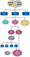 |
Fig. 1. Flow chart for creating the GRQ catalogue and the SRQ sample used for our analysis in this paper. Here, Kimball refers to the RLQ catalogue of Kimball et al. (2011), Paris to the Quasar catalogue of Pâris et al. (2018), Kuźmicz to the GRQ catalogue by Kuźmicz & Jamrozy (2021), and SAGAN-I to the GRG catalogue of Dabhade et al. (2020b). The ‘Others’ category consists of 19 sources with ambiguous morphology, 5 sources showing ghost emission due to artefacts, and 2 with false detection. The details of the steps illustrated here can be found in Sect. 2. |
2.3. The SRQ sample
In order to compare the properties of GRQs with SRQs, one needs to create a robust SRQ catalogue (size < 700 kpc). Hence, we compiled a sample of SRQs from the catalogue of K11, as described in Sect. 2.1. The K11 catalogue was compiled using optical data from the SDSS DR5 and the ancillary FIRST radio data. Hence, it is essential to update the redshifts from the latest products of SDSS (DR16), which have been revised over the years. We cross-matched the ‘triple’ category of 619 sources from the K11 catalogue with the robust quasar catalogue of Pâris et al. (2018). As a result, we have found a total of 616 RLQs to have reliable redshifts from Pâris et al. (2018). Of the 616 RLQs, 100 sources belong to the ‘unclassified’ or ‘X’ category as given by K11. Based on our analysis, we have identified 19 sources as having ambiguous radio morphology, 5 sources as having ghost emission (i.e. artefacts), and 2 sources as being wrongly classified, and 11 are found to be candidate Hybrid Morphology Radio Sources (HyMoRSs; Saikia et al. 1996; Gopal-Krishna & Wiita 2000). These 137 sources (100+19+5+2+11) are not being considered further in our study. However, we found 57 GRQs from the remaining 479 sources (47 are known, 10 are new), and hence, the final SRQ sample of 422 sources was formed. The above steps are illustrated in the form of a flow chart in Fig. 1.
3. Analysis
In this section we describe the methods used for computing various properties of the GRQ and SRQ samples.
3.1. Size
All ten new GRQs reported in this paper show FR-II radio morphology, as seen in the radio maps (Figs. 3 and 4). The projected linear size was measured as the distance between two hotspots (peak flux densities within 3 sigma contours) of lobes. The sizes are measured using the formula given in Sect. 3 of SAGAN.I. For the radio quasars in the SRQ sample, the FIRST radio maps were used for the measurement and confirmation of sizes. In the case of the sources in the GRQ catalogue, the angular sizes of 176 GRQs were estimated from the FIRST radio maps. For 17 GRQs, the angular sizes were taken from their respective reporting papers (Laing et al. 1983; de Bruyn 1989; Bhatnagar et al. 1998; Ishwara-Chandra & Saikia 1999; Schoenmakers et al. 2000a, 2001; Lara et al. 2001; Machalski et al. 2001, 2007; Saripalli et al. 2005; Hardcastle et al. 2016) as they had better maps than the FIRST. The sizes of the remaining 72 sources were measured using the LOFAR Two-meter Sky Survey (LoTSS; Shimwell et al. 2019; 18), TGSS ADR1 (25), and NVSS (29) radio images due to the unavailability of FIRST radio maps. The same method as described above was employed for all size measurements. All the radio sources considered in this paper belong to the FR-II class.
3.2. Radio core power
The radio core power (Pcore) of the SRQ sample was estimated at the rest-frame frequency of 1400 MHz from the observed core flux densities at 1400 MHz (FIRST) taken from K11 using the spectral index of 0 (Bridle et al. 1994; K11; Maithil et al. 2020). For sources in the GRQ catalogue, the core flux densities were obtained from the FIRST source catalogue (Helfand et al. 2015).
3.3. Total radio power
The integrated flux densities (entire source) at 150 MHz and 1400 MHz of the SRQs and the GRQs were measured from the TGSS and the NVSS radio maps, respectively, using CASA2 by selecting the regions of radio emission of the sources manually. For estimating the errors in the flux density measurements, we employed the method of Klein et al. (2003), considering 20% and 3% flux density calibration errors for the TGSS and NVSS, respectively. The total radio power at the respective rest-frame frequencies (P150 and P1400) was tabulated using the formula given in Sect. 3 of SAGAN.I.
3.4. Core dominance factor
The CDF is the ratio of core flux density (Score) to the extended flux density (Sext). The extended flux density is the flux density from the extended regions of the RLQ except from the core (e.g. lobes). It was estimated by subtracting the core flux density (measured from the FIRST) from the total integrated flux density (measured from the NVSS). The CDF was estimated at the rest-frame frequency (νrest) of 5000 MHz (or 5 GHz) for the sources. We derived the flux densities (both Score and Sext) at the 5 GHz rest-frame frequency from the respective flux densities observed at 1400 MHz (νobs) using the following formula:
 (1)
(1)
where Sνrest is the rest-frame flux density at νrest, and Sνobs is the observed flux density at νobs of the core and extended regions. The redshift is denoted by z for the source. Here, the spectral index, α, is assumed to be 0 and 0.75 (Dennett-Thorpe et al. 1999; Maithil et al. 2020) for the radio core and the extended emission, respectively. The CDF has also been referred to as ‘core fraction’ (fc), ‘core prominence’, and ‘radio core dominance’ in the literature. It is also often denoted as ‘R’.
3.5. Jet kinetic power
The jet kinetic power (QJet) is estimated from the low-frequency radio observations to avoid the effects of Doppler boosting, which is prominent in higher-frequency observations. For our analysis, it is measured using total radio power at 150 MHz from the TGSS maps, as described in Sect. 3 of SAGAN.I. For the GRQs in the GRQ catalogue taken from Dabhade et al. (2020a), the 144 MHz flux densities from the LoTSS were used to estimate the jet kinetic power.
3.6. Spectral index
The two-point spectral index ( ) was computed using the flux densities measured at 150 MHz (TGSS) and 1400 MHz (NVSS). For the sources that are either partially or not detected in the TGSS, we considered the spectral index to be 0.70 for both GRQs and SRQs. This is the median spectral index value of both the GRQ catalogue and the SRQ sample, which is used further for the estimation of the total radio powers.
3.7. Black hole mass
We cross-matched our GRQ catalogue and the SRQ sample with the SDSS-DR14 quasar catalogue made by Rakshit et al. (2020) to obtain the black hole masses (MBH), estimated using spectroscopic emission lines. Rakshit et al. (2020) used the emission lines of Hβ, MgII, and CIV for the redshift range of z < 0.8, 0.8 ≤ z < 1.9, and z ≥ 1.9, respectively. The black hole masses for 33 GRQs and 1 SRQ are not available from the catalogue of Rakshit et al. (2020). The MBH of 5 × 10⁷ M⊙ corresponds to a stellar velocity dispersion (σ) of 70 km s−1, which is the instrumental resolution limit of the SDSS spectra. Hence, only sources with masses above 5 × 10⁷ M⊙ were considered. We also took other quality filters recommended by Rakshit et al. (2020) into account while considering the MBH. Hence, 41 GRQs and 49 SRQs were not taken into account for analysing MBH and related properties.
3.8. Eddington ratio
The Eddington ratio (λEdd) of a source is related to the accretion rate of its supermassive black hole (SMBH). It is defined as the ratio of bolometric luminosity (Lbol) to the Eddington luminosity (LEdd) corresponding to its mass. Similar to MBH as described in Sect. 3.7, the Lbol was also obtained from the sample of Rakshit et al. (2020), who used the monochromatic line luminosity at 5100 Å, 3000 Å, and 1350 Å to estimate Lbol for the z range of z < 0.8, 0.8 ≤ z < 1.9, and z ≥ 1.9, respectively. We derived LEdd from MBH using the formula  ) erg s−1.
4. Results
The redshift (z) for the SRQ sample (422) ranges from 0.11 to 3.02, and for the GRQs (265) it ranges from 0.08 to 2.94. The redshift distributions of the final GRQ and SRQ samples are shown in Fig. 2a. The sample of GRQs has a mean redshift of about 0.91, whereas the distribution of SRQs has a mean value of 1.20. Figure 2b shows the distribution of GRQs and SRQs on the P − z (radio power – redshift) plane, where the radio power spans over three orders of magnitude. The non-availability of sources in the lower-right quadrant is due to Malmquist bias. It is observed that with the increase in redshift, the number of sources decreases. Most of the sources are populated around z ∼ 0.5 to 1.5. The most powerful GRQs, with radio power ∼1027 W Hz−1, are clustered between redshifts 1.0 and 2.0.
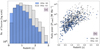 |
Fig. 2. Redshift distributions and relation with radio power. Left (a): redshift (z) distributions of all GRQs and SRQs. Right (b): all the GRQs and SRQs plotted on the P − z plane. The blue circles represent the GRQs and the plus signs the SRQs. The 1400 MHz NVSS flux density measurements were not available for two GRQs due to their position beyond the coverage area of the NVSS. For four SRQs, the flux densities at 1400 MHz are contaminated by the presence of other sources due to the low resolution of the NVSS. Therefore, (b) has 418 out of the 422 SRQs, and 263 out of the 265 GRQs. |
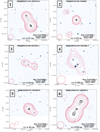 |
Fig. 3. Radio maps of the ten new GRQs (this page has numbers 1 to 6) as described in Sect. 2.1. The crimson contour represents the radio emission detected in the NVSS and black contours that from the FIRST survey. The background (blue) colour images are from the Pan-STARRS r band. In the lower-left corner, the beams of the NVSS and the FIRST are shown. The bottom middle of each image shows the angular scale for reference. The numbers in the upper-left corner represent the serial numbers from Table 1. Contour levels are at 3σ × [ − 1, 1, 1.4, 2.0, 2.8, 5.6, 11.2, 22.4] for the NVSS and 3σ × [ − 1, 1.4, 2.0, 2.8, 5.6, 11.2, 22.4] for the FIRST, where dashed contours represent negative values. The typical σ values for the FIRST and the NVSS are 0.15 and 0.45 mJy beam−1, respectively. |
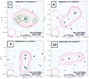 |
Fig. 4. Same as in Fig. 3, but for GRQ numbers 7−10, as described in Sect. 2.1. In the case of GRQ 7 (or GRQ J132217.27+294551.3), the radio emission from the TGSS is shown in green contours for clarity of the source morphology, where the σ is 2.7 mJy beam−1 and six contours levels are drawn above 3σ. |
Our aim is to understand how different or similar the SRQ and GRQ populations are in terms of their optical and radio properties, and under what conditions the SRQs grow into GRQs. To achieve this, we studied the samples by comparing properties in redshift-matched sub-samples. In this method, we divided the samples into two redshift bins depending on the median values of the entire z distributions. The median value of the GRQ sample is 0.82, whereas the median z value for the SRQ sample is 1.16. We considered the average of these two median values (z = 1.00) to divide the GRQ and SRQ sample into two bins. Both the bins – the lower one (z ≤ 1.00) and the upper one (1.00 < z ≤ 2.45) – are matched in redshift with a Kolmogorov–Smirnov (K-S) test p value and a Wilcoxon-Mann-Whitney (WMW) test p value for the lower bin being 0.23 and 0.05 and for the upper bin being 0.11 and 0.05, respectively. Figures 5a and 6a show the respective distributions.
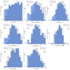 |
Fig. 5. Properties of the redshift-matched samples (z ≤ 1.00), where GRQs and SRQs are represented in unhatched and hatched bins, respectively. The mean and median values of the distributions are given in Table 2. Panel a: redshift distributions for z ≤ 1.00; Panel b: distributions of radio core power (Pcore) at 1400 MHz obtained from the FIRST; Panel c: distributions of the CDF; Panel d: distributions of total radio power (P1400) at 1400 MHz obtained from the NVSS; Panel e: distributions of jet kinetic power (QJet); Panel f: distributions of spectral index ( |

Based on the above method, we compared properties of GRQs and SRQs, such as Pcore, CDF, P1400, QJet,  , MBH, and λEdd, as discussed in Sect. 3. The results are summarised in Table 2, where we have provided the statistics related to all sub-samples with respect to their properties, such as the mean, median, and the p values of the statistical tests. We reject the null hypothesis that the two samples were drawn from the same distribution if the p value is less than the significance level.
Mean and median values of properties for comparison between GRQs and SRQs.
4.1. Distributions of radio core power
The Pcore distributions of GRQs and SRQs are shown in Fig. 5b for the lower redshift bin and in Fig. 6b for the upper redshift bin. Both distributions show that the SRQs have higher Pcore than the GRQs. This is supported by the p values of statistical tests given in Table 2. The Pcore of SRQs is found to be more than twice that of GRQs.
4.2. Distributions of core dominance factor
The radio cores of powerful radio-loud AGN (e.g. quasars) are Doppler boosted due to relativistic beaming (Blandford & Königl 1979; Scheuer & Readhead 1979; Orr & Browne 1982; Kapahi & Saikia 1982) if the source axis is close to our line of sight. Hence, the CDF can act as an independent statistical estimator of the orientation of the sources (Wills & Brotherton 1995; Marin & Antonucci 2016). The CDF distributions of SRQs and GRQs for both redshift-matched samples are shown in Figs. 5c and 6c for the lower and upper redshift bins, respectively. The range of CDF values of SRQs and GRQs are consistent with the findings of previous studies (Browne & Murphy 1987; Marin & Antonucci 2016; Maithil et al. 2020). We find that the CDF of SRQs is more than that of GRQs by a factor of nearly two for both redshift-matched samples. This implies that radio cores of SRQs appear more powerful than GRQs, which is also seen in Sect. 4.1. It may be relevant to note here that for galaxies alone, which are believed to be inclined at large angles to the line of sight in the unification scheme, Ishwara-Chandra & Saikia (1999) did not find any significant difference in the degree of core prominence between GRGs and smaller ones when they are matched in total radio luminosity.
4.3. Distributions of total radio power
The distributions of P1400 for SRQs and GRQs for redshift-matched samples are shown in Figs. 5d and 6d for lower and upper bins, respectively. Similar to the Pcore and CDF, the trend for P1400 is also the same, with SRQs being more powerful than GRQs.
4.4. Distributions of jet kinetic power
The QJet shows no exception to the earlier three properties, as reflected in Figs. 5e and 6e for the lower and upper bins of redshift-matched samples and the statistical test results tabulated in Table 2. This indicates that SRQs have more powerful jets as compared to GRQs.
4.5. Distributions of the spectral index
The  distributions for GRQs and SRQs are found to be similar for both the lower and upper bins of redshift-matched samples. The distributions of
  are shown in Fig. 5f for the lower bin and in Fig. 6f for the upper bin. Analogous to SRGs and GRGs (Dabhade et al. 2020b), the SRQs and GRQs have similar spectral index values.
4.6. Distributions of black hole mass
The distributions of MBH for redshift-matched samples are shown in Figs. 5g and 6g for the lower and upper bins, respectively. The MBH of GRQs is found to be similar to that of SRQs. This result is in line with the case of GRGs and SRGs (Dabhade et al. 2020b), where the black hole masses of GRGs and SRGs have similar distributions that peak at similar values. Moreover, if we compare the MBH of GRGs and SRGs (Table 3 of SAGAN.I and our Fig. 8) with that of GRQs and SRQs, we notice that the black holes of the latter population are more massive than those of the former.
4.7. Distributions of Eddington ratio
The results of comparing the distributions of the Eddington ratios of GRQs and SRQs are found to be on similar lines with those of the GRGs and SRGs (Dabhade et al. 2020b). This accounts for the fact that SRQs have higher λEdd than GRQs, similar to SRGs when compared to GRGs. The λEdd distributions for SRQs and GRQs can be seen in Figs. 5h and 6h for the lower and upper bins of redshift-matched samples, respectively. When we compare GRGs and SRGs with GRQs and SRQs, it is interesting to find that the λEdd of the galaxy population is less than that of the quasar population (see Table 3 of SAGAN.I and our Fig. 8).
5. Discussion
In this section we discuss our results in detail and provide a possible model for GRQ growth.
5.1. CDF-size relation
As per the relativistic beaming model (Blandford & Königl 1979), the radio core emission is significantly enhanced with respect to the extended components when observed from an angle close to the line of sight in comparison to a larger viewing angle. Hence, the CDF could be a statistical measure of the inclination of the jet axis with respect to the line of sight. As per the AGN orientation unification scheme, the CDF is expected to be anti-correlated with projected linear sizes of the sources; in other words, sources with larger linear sizes should have less prominent cores, as shown first in Kapahi & Saikia (1982). This is evident in Fig. 7, where it can be observed that SRQs have more prominent cores as compared to GRQs. It is suggested in the literature (e.g. Gopal-Krishna et al. 1989) that giant radio sources have higher core prominence as compared to smaller radio sources, implying that the former have stronger nuclear activity. Our analysis shows that the CDF of SRQs is almost twice that of GRQs in both bins of redshift-matched samples. This is largely due to the beaming effect in which SRQs, on average, are viewed at smaller angles to the line of sight compared to GRQs.
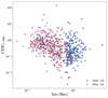 |
Fig. 7. CDF shown as a function of the size of RLQs. We observe a trend of decreasing CDF as the size of the source increases, possibly showing the effect of Doppler boosting. |
5.2. Role of black hole mass and Eddington ratio
In SAGAN.I, we presented the results of the MBH and λEdd properties of giants, with AGN (non-quasars) having both low and high excitation types, and it was found that the high excitation giant radio galaxies (HEGRGs) have higher λEdd than the low excitation giant radio galaxies (LEGRGs). A small overlap of λEdd was observed for HEGRGs and LEGRGs; this has also been observed for the small-sized RGs (Whittam et al. 2018), although they are thought to have a bi-modal distribution, as seen in the work of Best & Heckman (2012). The MBH distributions were found to be similar for SRGs and GRGs in SAGAN.I.
In order to investigate the role of MBH and λEdd in the exceptionally large size of radio galaxies and quasars, we considered the samples from SAGAN.I in addition to our SRQ-GRQ samples for comparative study. To compare properties (MBH and λEdd) of GRGs, SRGs, GRQs, and SRQs, we opted to use box plots, as seen in Fig. 8, instead of the traditional histograms.
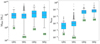 |
Fig. 8. Box plots as described in Sect. 5.2, which show distributions of black hole mass (left) and Eddington ratio (right) for GRGs, SRGs, SRQs, and GRQs. The number shown in the green box represents the number of sources in each sample. The solid red line indicates the median of the distribution, and the dashed purple line denotes the mean. |
Box plots (Tukey 1977) are also known as box and whisker diagrams or plots with outliers. Here, the upper and lower ends of the box represent the upper and lower quartiles, respectively, for a dataset. The two lines extending from the box are known as whiskers, which indicate variability outside the upper and lower quartiles. The dots are the outliers in the dataset, and the line in the middle of the box represents the median of the sample. They represent a graphical method that is better for showing variations in a dataset and for an analysis consisting of multiple datasets.
In Fig. 8 we can see the box plot illustrating the distributions of MBH and λEdd of GRGs and SRGs (non-quasar hosts) as well as GRQs and SRQs. In order to avoid possible problems with redshift evolution, we only considered objects matched in redshift, and hence, the sample is restricted below the redshift of 1. For MBH we observe significant overlap between GRGs and GRQs, with GRQs tending to have higher MBH than GRGs, and the giants having marginally higher values of MBH than smaller sources for both galaxies and quasars. However, a clear bi-modal distribution or contrasting difference is observed for λEdd, with negligible overlap. Also, this result indicates a higher accretion rate for the giants with quasar hosts or GRQs compared with GRGs; a similar result is seen for their smaller-sized counterparts (SRGs and SRQs). Although the smaller sources appear to have marginally higher values of λEdd for both galaxies and quasars, it can be seen that λEdd does not depend strongly on the size of radio-loud AGN. Now, having shown this result observationally, we can investigate other properties of SRGs and SRQs and GRGs and GRQs, which could provide us further clues as to their giant sizes (e.g. environment).
5.3. Disc-jet coupling in radio quasars
Extragalactic radio jets of various shapes and sizes have been known for nearly five decades (Hardcastle & Croston 2020). New observations and numerical simulations have revealed new information and help in the quest for understanding the launching and collimation of astrophysical jets. The recipe of jet launching involves accretion, magnetic field, and spin, but it is still not properly understood how an accretion disc gives rise to ordered collimated outflows. According to the Blanford–Znajek mechanism (Blandford & Znajek 1977), spin and magnetic flux threading the horizon determine the jet power. One of the possible ways to understand this is to explore the disc-jet symbiosis (Falcke & Biermann 1995; Willott et al. 1999; Merloni et al. 2003; Fender 2010). The disc-jet connection depicts an interlink between the accretion process (rate, mode, field geometry, and strength) and the power output or jets (McNamara & Nulsen 2007; Fender 2010; Stepanovs & Fendt 2016), where the jets are rooted in the nuclear region of the accretion disc and move along the axis of rotation, a phenomenon also known as disc-jet coupling. Some of the earliest observational evidence was given by Rawlings & Saunders (1991) through a correlation between jet power and the disc luminosity indicator for FR-II RGs. Cao & Jiang (1999) confirmed this via probing the correlation between radio luminosity at 5 GHz and broad-line emission (an indicator for accretion power) for RLQs. Several other studies have also confirmed the inter-connection between discs and jets, via monitoring the X-ray and optical variability, by exploring the radio–X-ray correlation for RG 3C 120 (Marscher et al. 2002; Chatterjee et al. 2009), or through the correlation observed between broad-line region (BLR) luminosity and jet power traced using γ-ray luminosity for blazars and radio luminosity for RGs (Sbarrato et al. 2014).
Recently, the Event Horizon Telescope (EHT) collaboration (Event Horizon Telescope Collaboration 2021) has imaged the polarised emission of the swirling plasma in the event horizon of the SMBH of Messier 87. The EHT observations of M 87 along with favouring results from simulations indicate that the magnetic fields near the event horizon are dynamically important and play a crucial role in the formation of jets (Blandford & Znajek 1977; Narayan & Yi 1994; Tchekhovskoy et al. 2011; Davis & Tchekhovskoy 2020) and in the physics (Hawley & Balbus 1991; Davis & Tchekhovskoy 2020) of the accretion disc.
As the magnetic field lines encompassing the black hole build up near the event horizon, this gives rise to a magnetically arrested disc (MAD) scenario (Narayan et al. 2003; Tchekhovskoy et al. 2011). It affects the disc properties and hinders the gas infall into the accreting black hole. The magnetic flux in the rotating disc is so intense that the magnetic field lines are piled up and twisted in the direction perpendicular to the plane of the accretion disc (Zamaninasab et al. 2014), leading to the launching and collimation of jets. Zamaninasab et al. (2014) have shown that the magnetic field strength in jets strongly scales with accretion disc luminosity (Lbol). Taking Lbol as a proxy for magnetic flux in the jet-launching site, the Lbol − QJet correlation indicates the contribution of the magnetic field in powering jets, which in turn hints at the disc-jet coupling. Based on our results, we find strong evidence of a disc-jet interplay for our sample of SRQs and GRQs (or RLQs broadly speaking), as shown in Fig. 9a, where Lbol, representing accretion disc luminosity, is plotted as a function of QJet. Spearman’s correlation coefficient of 0.55 supports this scenario. Part of the scatter in the plot could be due to either measurement uncertainties or radiative loss due to the interaction of the jet with its immediate environment. Another factor, in addition to the accretion phenomenon contributing to jet kinetic power, could be the possible contribution of spin (van Velzen & Falcke 2013).
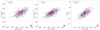 |
Fig. 9. Correlations between Lbol and QJet in sub-figure (a), Lbol and Pcore in sub-figure (b), and λEdd and Eddington scaled Pcore in sub-figure (c) for GRQs and SRQs. The Spearman’s correlation coefficients are 0.55, 0.65, and 0.70, respectively. |
In SAGAN.I, a similar correlation was found for a relatively small sample of GRGs, confirming the close interlink between the disc properties and the collimated jetted output of SMBHs. We find that nearly 10% of the accretion luminosity of GRQs and SRQs contributes to the jet kinetic power as given by the coupling parameter QJet ≡ QJet/Lbol = 0.09; this is significantly lower than the findings of Willott et al. (1999), who reported QJet to be 20%. Moreover, our study sample has five SRQs and two GRQs with QJet > 1. Based on the study by Ghisellini et al. (2014), QJet > 1 is a plausible astrophysical scenario, as they have shown for flat spectrum radio quasars (FSRQs) or BL Lac objects. They measured jet power from γ-ray luminosity and found that relativistic jets have more power than the luminosity of the accretion disc. Such a scenario can be explained when the extraction of spin energy from a black hole (Tchekhovskoy et al. 2011) is invoked along with disc-jet coupling. The higher spin values for jet production in RLQs have also been suggested by other studies (Schulze et al. 2017; Chen et al. 2021).
In addition, we also examined the possible correlation between Lbol and Pcore (Fig. 9b) and found them to have a strong correlation with a Spearman’s correlation coefficient of 0.65. When normalised to LEdd, the resulting correlation of λEdd as a function of Pcore/LEdd gets even stronger, with a correlation coefficient of 0.7 (Fig. 9c). Due to the resolution limit (5″), the radio emission of the nuclear region (or radio core) that we are addressing here possibly includes parsec-scale jets in some sources. Therefore, this relation provides another piece of evidence for the contribution of the accretion properties of the SMBH in fueling the relativistic radio jets. The sub-plots of Fig. 9 give a clearer view of how the disc magnetic field affects the formation of relativistic jets. The high Eddington ratio (accretion rate) leads to a higher accumulation of magnetic fields in the vicinity of the black hole, and, once the magnetic field reaches the saturation state, the magneto-rotational instabilities are triggered. This process carries away the angular momentum of the disc into a jetted outflow. The spin plays the role of twisting the magnetic field lines and confirms the transfer of magnetic energy into the Poynting flux of relativistic jets.
Lastly, there have been studies suggesting the possible contribution of relativistic beaming affecting the optical continuum emission in quasars. However, recent studies by Van Gorkom et al. (2015) have shown that such a contribution is negligible.
5.4. SRQ to GRQ
In this decade, the arrival of new sensitive instruments and the advancement in software has facilitated the discovery of a larger sample of GRGs, especially the ones with low surface brightness (e.g. Dabhade et al. 2020a; Delhaize et al. 2021). However, the question about the conditions under which an SRG or an SRQ becomes a giant remains to be well understood. In an effort to answer this question, we carried out a comparative study between the properties of GRQs and SRQs. In Sect. 4, distributions of properties concerning the host and large-scale properties of GRQs and SRQs are discussed. Our results show that SRQs have more prominent cores as compared to GRQs. They have a Pcore and a CDF twice as large as those of GRQs. Similarly, for large-scale properties such as P1400 and QJet, SRQs tend to show more powerful jets that carry almost double the radio power than the GRQs. However, interestingly, and irrespective of SRQs appearing to be more powerful, the spectral index distributions of both SRQs and GRQs are observed to be the same. This indicates that the AGN activity in the GRQs has not ceased. Owing to their larger sizes, GRQs are more susceptible to higher radiation losses due to adiabatic expansion and inverse Compton scattering and yet have similar spectral indices between about 150 and 1400 MHz. This indicates that the AGN activity is perhaps more dominant or prolonged than that of SRQs. It should be noted that the re-acceleration of radiating particles in the jets and lobes can also lead to flatter spectral indices.
If we consider the samples in the lower and upper redshift bins, it is observed that sources at high redshifts are more powerful. This is because with the increase in redshift there is a decrease in the detection of less powerful sources due to Malmquist bias. It is also noticed that sources in the upper bin (high z) have steeper spectra. This could possibly be the consequence of the radio luminosity–spectral index (P − α) correlation, where sources with high radio power are observed to have steeper spectral indices (Blundell et al. 1999; Dabhade et al. 2020b). Sources with high QJet have enhanced magnetic fields in the hotspots. This eventually results in the rapid cooling of relativistic electrons, and, as a result, electrons with steeper spectra are injected into the lobes.
The black hole mass distributions of both SRQs and GRQs are found to be statistically similar, although the former are accreting faster than the latter, which is reflected in their higher values of λEdd. Based on our analysis, we suggest the following basic model for the growth and evolution of GRQs: the GRQ progenitor is an SRQ with a high accretion rate, which grows with time in terms of overall size. This is supported by the self-regulated black hole growth scenario (Hopkins et al. 2005a,b), where it is shown that the feedback energy from the AGN can heat up gas in the host galaxy and result in the quenching of the accretion process. This in turn will lead to a decrease in the λEdd. Hence, this could lead to a reduction in the overall output from the disc and affect the jet power. Our results presented in Sect. 4 show that Pcore, QJet, P1400, and λEdd are lower for GRQs compared with SRQs, which is consistent with the above model. This can be tested by comparing the ‘effective’ lifetimes (Hopkins & Hernquist 2009) of the quasars with the spectral and dynamical ages of the SRQs and GRQs. The measurement of spectral and dynamical ages of large samples of SRQs and GRQs via multi-frequency radio observations is quite difficult owing to the large time requirements. Spectral age measurements of a few quasars (Parma et al. 1999) indicate their ages to be in the range of ∼1−20 Myr, which is comparable to the quasar lifetimes obtained in the studies of Hopkins et al. (2005a).
The signs of restarted radio AGN (Saikia & Jamrozy 2009) based on radio morphology were revealed with the discovery of ‘double-double radio galaxies’ (Schoenmakers et al. 2000b) nearly two decades ago; only about 110 such sources are known so far. However, only a very few have quasar hosts (e.g. 4C 02.27 or J0935+0204 Jamrozy et al. 2009, J0746+4526 Nandi et al. 2014, J1244+5941 Saikia & Jamrozy 2009), indicating their rarity. Also, there are only a few examples of RLQs with intermittent jet activity (e.g. PKS 1127–145 Siemiginowska et al. 2007; 3C 273 Stawarz 2004). Hence, it is possible that SRQs and GRQs have episodic activity on a very short timescale, which seldom manifests as the double-double morphology for us to observe.
5.5. High redshift GRQs
The radio emission from radio sources is quenched due to enhanced inverse Compton losses against the cosmic microwave background (CMB) for higher redshift sources. For a radio-loud AGN that has grown to larger volumes over a period of a relatively long time, the internal magnetic energy density in the radio lobes is expected to be less than the energy density of the CMB photons. This was clearly demonstrated by Ishwara-Chandra & Saikia (1999) for their sample of giant and smaller sources. In such scenarios, the relativistic radio-emitting electrons will preferentially lose energy via inverse Compton collisions with the CMB photons. This will lead to enhanced X-ray emission and the suppression of radio emission. The hotspots in the lobes are relatively less affected by this due to their compactness and higher magnetic energy density. There is a (1 + z)4 factor dependence of the CMB energy density, and hence, for high redshifts, the quenching of radio emission is expected to be much larger. Therefore, at higher redshift, inverse Compton ghosts of radio galaxies or radio quasars (Mocz et al. 2011) are observed, where the jets of such sources have switched off and the lobes are visible in X-ray only (e.g. Tamhane et al. 2015).
In our GRQ catalogue we have eight high-z sources with 2 < z ≤ 2.94 that have radio powers of ∼1027 W Hz−1 at 1400 MHz. The radio maps reveal their FR-II radio morphologies, indicating that these GRQs must be enormously powerful to negate the quenching effect of the high-z CMB. Studies (Mocz et al. 2011; Fabian et al. 2014; Ghisellini et al. 2015) have shown the existence of double-lobed radio sources at higher redshifts, though not for sources of megaparsec sizes. Recently, Bañados et al. (2021) discovered the farthest RLQ, at a redshift of 6.82, which is when the age of the Universe was only ∼0.8 Gyr. These studies have shown the existence of radio jetted AGN at higher redshifts or when the Universe was in its early stages, where black holes managed to grow to supermassive sizes. It is possible that a population of such sources is currently invisible to us due to the sensitivity limits and, hence, are prime targets for future telescopes such as the Square Kilometre Array (SKA) and Athena. Based on the best current data available (radio and optical), only 3 of the total 200 quasars known above the redshift of 6 are radio-loud (Bañados et al. 2021). High-z radio-loud AGN are often found in over-dense environments and, hence, also are tracer of protoclusters (Venemans et al. 2007; Wylezalek et al. 2013; Hatch et al. 2014), which could be the progenitors of the present-day galaxy clusters. It is vital to study these objects as they are probes of the high redshift Universe and their study holds the key to understanding the formation, growth, and evolution of radio sources.
6. Summary
The results of our study and analysis are summarised as follows:
-
We report the discovery of ten new GRQs in the redshift range of 0.66−1.72, with the largest one having a projected linear size of 1.55 Mpc. All of them have an FR-II type radio morphology.
-
We have constructed a GRQ catalogue that consists of 121 sources from Dabhade et al. (2020b) and 134 sources from Kuźmicz & Jamrozy (2021), in addition to our 10 new GRQs. We also created a well-defined SRQ sample of 422 sources selected from Kimball et al. (2011).
-
To understand how similar GRQs and SRQs are, we have compared their various properties, such as Pcore, CDF, P1400, QJet,
 , MBH, and λEdd. For samples in the redshift-matched bins, we found that SRQs have higher Pcore, CDF, P1400, QJet, and λEdd as compared to GRQs. But in the case of MBH and
  , they both show similar distributions. The higher values of the CDF suggest that, statistically, the SRQs are inclined at smaller angles to the line of sight than the GRQs.
 -
Our results show that the central engines of SRQs are more powerful than those in GRQs.
-
When compared to GRGs and SRGs, the GRQs and SRQs have higher MBH and λEdd, indicating that quasar engines are more active.
-
We find tight correlations between Lbol and QJet and between Lbol and Pcore. This implies that the disc-jet coupling has a significant contribution towards launching jets.
-
The λEdd distributions of both GRGs and GRQs and SRGs and SRQs are bi-modal, with the quasars having significantly higher values of λEdd. The smaller sources appear to have marginally higher values of λEdd for both galaxies and quasars, suggesting only small changes in the accretion process as radio sources grow to their giant sizes.
In the coming time, spectroscopic optical data via new surveys will enable us to find more GRQs with wider multi-wavelength data coverage and hence will allow us to study them in more depth.
Search & Analysis of Giant radio galaxies with Associated Nuclei.
Common Astronomy Software Applications (CASA; McMullin et al. 2007) task ‘CASA-VIEWER’.
Acknowledgments
We thank the anonymous reviewer for critically reading the manuscript and providing with valuable comments. We thank IUCAA (especially Radio Physics Lab. (http://www.iucaa.in/~rpl/)), Pune for providing all the facilities during the period the work was carried out. M.M. would like to dedicate this paper in the loving memory of her father (Mr. Shakti Pada Mahato). L.C.H. was supported by the National Key R&D Program of China (2016YFA0400702) and the National Science Foundation of China (11721303, 11991052). We gratefully acknowledge the use of Edward (Ned) Wright’s online Cosmology Calculator. This research has made use of the VizieR catalogue tool, CDS, Strasbourg, France (Ochsenbein et al. 2000). This research has made use of the CIRADA cutout service at URL (http://cutouts.cirada.ca), operated by the Canadian Initiative for Radio Astronomy Data Analysis (CIRADA). CIRADA is funded by a grant from the Canada Foundation for Innovation 2017 Innovation Fund (Project 35999), as well as by the Provinces of Ontario, British Columbia, Alberta, Manitoba and Quebec, in collaboration with the National Research Council of Canada, the US National Radio Astronomy Observatory and Australia’s Commonwealth Scientific and Industrial Research Organisation. We acknowledge that this work has made use of ASTROPY (Astropy Collaboration 2013), APLPY (Robitaille & Bressert 2012), MATPLOTLIB (Hunter 2007) and TOPCAT (Taylor 2005).
References
- Amirkhanyan, V. R. 2016, Astrophys. Bull., 71, 384 [NASA ADS] [CrossRef] [Google Scholar]
- Astropy Collaboration (Robitaille, T. P., et al.) 2013, A&A, 558, A33 [NASA ADS] [CrossRef] [EDP Sciences] [Google Scholar]
- Bañados, E., Mazzucchelli, C., Momjian, E., et al. 2021, ApJ, 909, 80 [CrossRef] [Google Scholar]
- Bassani, L., Ursini, F., Malizia, A., et al. 2021, MNRAS, 500, 3111 [Google Scholar]
- Beaklini, P. P. B., Quadros, A. V. C., de Avellar, M. G. B., Dantas, M. L. L., & Cançado, A. L. F. 2020, MNRAS, 497, 1463 [NASA ADS] [CrossRef] [Google Scholar]
- Becker, R. H., White, R. L., & Helfand, D. J. 1995, ApJ, 450, 559 [Google Scholar]
- Best, P. N., & Heckman, T. M. 2012, MNRAS, 421, 1569 [NASA ADS] [CrossRef] [Google Scholar]
- Bhatnagar, S., Gopal-Krishna, & Wisotzki, L. 1998, MNRAS, 299, L25 [NASA ADS] [CrossRef] [Google Scholar]
- Blandford, R. D., & Königl, A. 1979, ApJ, 232, 34 [Google Scholar]
- Blandford, R. D., & Znajek, R. L. 1977, MNRAS, 179, 433 [NASA ADS] [CrossRef] [Google Scholar]
- Blundell, K. M., Rawlings, S., & Willott, C. J. 1999, AJ, 117, 677 [Google Scholar]
- Bridle, A. H., & Perley, R. A. 1984, ARA&A, 22, 319 [NASA ADS] [CrossRef] [Google Scholar]
- Bridle, A. H., Hough, D. H., Lonsdale, C. J., Burns, J. O., & Laing, R. A. 1994, AJ, 108, 766 [NASA ADS] [CrossRef] [Google Scholar]
- Browne, I. W. A., & Murphy, D. W. 1987, MNRAS, 226, 601 [NASA ADS] [Google Scholar]
- Cao, X., & Jiang, D. R. 1999, MNRAS, 307, 802 [NASA ADS] [CrossRef] [Google Scholar]
- Chatterjee, R., Marscher, A. P., Jorstad, S. G., et al. 2009, ApJ, 704, 1689 [NASA ADS] [CrossRef] [Google Scholar]
- Chen, Y., Gu, Q., Fan, J., et al. 2021, ApJ, 913, 93 [NASA ADS] [CrossRef] [Google Scholar]
- Cirasuolo, M., Magliocchetti, M., Celotti, A., & Danese, L. 2003, MNRAS, 341, 993 [NASA ADS] [CrossRef] [Google Scholar]
- Condon, J. J., Cotton, W. D., Greisen, E. W., et al. 1998, AJ, 115, 1693 [Google Scholar]
- Dabhade, P., Röttgering, H. J. A., Bagchi, J., et al. 2020a, A&A, 635, A5 [NASA ADS] [CrossRef] [EDP Sciences] [Google Scholar]
- Dabhade, P., Mahato, M., Bagchi, J., et al. 2020b, A&A, 642, A153 [NASA ADS] [CrossRef] [EDP Sciences] [Google Scholar]
- Dabhade, P., Combes, F., Salomé, P., Bagchi, J., & Mahato, M. 2020c, A&A, 643, A111 [NASA ADS] [CrossRef] [EDP Sciences] [Google Scholar]
- Davis, S. W., & Tchekhovskoy, A. 2020, ARA&A, 58, 407 [Google Scholar]
- de Bruyn, A. G. 1989, A&A, 226, L13 [NASA ADS] [Google Scholar]
- Delhaize, J., Heywood, I., Prescott, M., et al. 2021, MNRAS, 501, 3833 [Google Scholar]
- Dennett-Thorpe, J., Bridle, A. H., Laing, R. A., & Scheuer, P. A. G. 1999, MNRAS, 304, 271 [NASA ADS] [CrossRef] [Google Scholar]
- Event Horizon Telescope Collaboration (Akiyama, K., et al.) 2021, ApJ, 910, L13 [Google Scholar]
- Fabian, A. C., Walker, S. A., Celotti, A., et al. 2014, MNRAS, 442, L81 [NASA ADS] [CrossRef] [Google Scholar]
- Falcke, H., & Biermann, P. L. 1995, A&A, 293, 665 [NASA ADS] [Google Scholar]
- Fanaroff, B. L., & Riley, J. M. 1974, MNRAS, 167, 31P [Google Scholar]
- Fender, R. 2010, in ‘Disc-Jet’ Coupling in Black Hole X-ray Binaries and Active Galactic Nuclei, ed. T. Belloni, 794, 115 [Google Scholar]
- Ghisellini, G., Tavecchio, F., Maraschi, L., Celotti, A., & Sbarrato, T. 2014, Nature, 515, 376 [NASA ADS] [CrossRef] [Google Scholar]
- Ghisellini, G., Haardt, F., Ciardi, B., et al. 2015, MNRAS, 452, 3457 [Google Scholar]
- Gopal-Krishna, & Wiita, P. J. 2000, A&A, 363, 507 [Google Scholar]
- Gopal-Krishna, Wiita, P. J., & Saripalli, L. 1989, MNRAS, 239, 173 [NASA ADS] [CrossRef] [Google Scholar]
- Hardcastle, M. J., & Croston, J. H. 2020, New Astron. Rev., 88, 101539 [Google Scholar]
- Hardcastle, M. J., Gürkan, G., van Weeren, R. J., et al. 2016, MNRAS, 462, 1910 [Google Scholar]
- Hatch, N. A., Wylezalek, D., Kurk, J. D., et al. 2014, MNRAS, 445, 280 [NASA ADS] [CrossRef] [Google Scholar]
- Hawley, J. F., & Balbus, S. A. 1991, ApJ, 376, 223 [NASA ADS] [CrossRef] [Google Scholar]
- Hazard, C., Mackey, M. B., & Shimmins, A. J. 1963, Nature, 197, 1037 [NASA ADS] [CrossRef] [Google Scholar]
- Helfand, D. J., White, R. L., & Becker, R. H. 2015, ApJ, 801, 26 [NASA ADS] [CrossRef] [Google Scholar]
- Hintzen, P., Ulvestad, J., & Owen, F. 1983, AJ, 88, 709 [NASA ADS] [CrossRef] [Google Scholar]
- Hopkins, P. F., & Hernquist, L. 2009, ApJ, 698, 1550 [NASA ADS] [CrossRef] [Google Scholar]
- Hopkins, P. F., Hernquist, L., Martini, P., et al. 2005a, ApJ, 625, L71 [Google Scholar]
- Hopkins, P. F., Hernquist, L., Cox, T. J., et al. 2005b, ApJ, 630, 705 [NASA ADS] [CrossRef] [Google Scholar]
- Hunter, J. D. 2007, Comput. Sci. Eng., 9, 90 [NASA ADS] [CrossRef] [Google Scholar]
- Intema, H. T., Jagannathan, P., Mooley, K. P., & Frail, D. A. 2017, A&A, 598, A78 [NASA ADS] [CrossRef] [EDP Sciences] [Google Scholar]
- Ishwara-Chandra, C. H., & Saikia, D. J. 1999, MNRAS, 309, 100 [NASA ADS] [CrossRef] [Google Scholar]
- Jamrozy, M., Saikia, D. J., & Konar, C. 2009, MNRAS, 399, L141 [NASA ADS] [CrossRef] [Google Scholar]
- Jiang, L., Fan, X., Ivezić, Ž., et al. 2007, ApJ, 656, 680 [Google Scholar]
- Kapahi, V. K., & Saikia, D. J. 1982, JApA, 3, 465 [NASA ADS] [Google Scholar]
- Kellermann, K. I., Condon, J. J., Kimball, A. E., Perley, R. A., & Ivezić, Ž. 2016, ApJ, 831, 168 [Google Scholar]
- Kimball, A. E., Ivezić, Ž., Wiita, P. J., & Schneider, D. P. 2011, AJ, 141, 182 [NASA ADS] [CrossRef] [Google Scholar]
- Klein, U., Mack, K.-H., Gregorini, L., & Vigotti, M. 2003, A&A, 406, 579 [NASA ADS] [CrossRef] [EDP Sciences] [Google Scholar]
- Kozieł-Wierzbowska, D., & Stasińska, G. 2011, MNRAS, 415, 1013 [CrossRef] [Google Scholar]
- Kuźmicz, A., & Jamrozy, M. 2012, MNRAS, 426, 851 [CrossRef] [Google Scholar]
- Kuźmicz, A., & Jamrozy, M. 2021, ApJS, 253, 25 [CrossRef] [Google Scholar]
- Kuźmicz, A., Jamrozy, M., Bronarska, K., Janda-Boczar, K., & Saikia, D. J. 2018, ApJS, 238, 9 [Google Scholar]
- Kuźmicz, A., Czerny, B., & Wildy, C. 2019, A&A, 624, A91 [NASA ADS] [CrossRef] [EDP Sciences] [Google Scholar]
- Lacy, M., Baum, S. A., Chandler, C. J., et al. 2020, PASP, 132, 035001 [Google Scholar]
- Laing, R. A., Riley, J. M., & Longair, M. S. 1983, MNRAS, 204, 151 [NASA ADS] [CrossRef] [Google Scholar]
- Lara, L., Cotton, W. D., Feretti, L., et al. 2001, A&A, 370, 409 [NASA ADS] [CrossRef] [EDP Sciences] [Google Scholar]
- Machalski, J., Jamrozy, M., & Zola, S. 2001, A&A, 371, 445 [NASA ADS] [CrossRef] [EDP Sciences] [Google Scholar]
- Machalski, J., Koziel-Wierzbowska, D., & Jamrozy, M. 2007, Acta Astron., 57, 227 [NASA ADS] [Google Scholar]
- Maithil, J., Runnoe, J. C., Brotherton, M. S., et al. 2020, ApJ, 904, 179 [NASA ADS] [CrossRef] [Google Scholar]
- Marin, F., & Antonucci, R. 2016, ApJ, 830, 82 [NASA ADS] [CrossRef] [Google Scholar]
- Marscher, A. P., Jorstad, S. G., Gómez, J.-L., et al. 2002, Nature, 417, 625 [NASA ADS] [CrossRef] [Google Scholar]
- McMullin, J. P., Waters, B., Schiebel, D., Young, W., & Golap, K. 2007, in Astronomical Data Analysis Software and Systems XVI, eds. R. A. Shaw, F. Hill, & D. J. Bell, ASP Conf. Ser., 376, 127 [Google Scholar]
- McNamara, B. R., & Nulsen, P. E. J. 2007, ARA&A, 45, 117 [NASA ADS] [CrossRef] [Google Scholar]
- Merloni, A., Heinz, S., & di Matteo, T. 2003, MNRAS, 345, 1057 [Google Scholar]
- Mocz, P., Fabian, A. C., & Blundell, K. M. 2011, MNRAS, 413, 1107 [NASA ADS] [CrossRef] [Google Scholar]
- Nandi, S., Roy, R., Saikia, D. J., et al. 2014, ApJ, 789, 16 [NASA ADS] [CrossRef] [Google Scholar]
- Narayan, R., & Yi, I. 1994, ApJ, 428, L13 [Google Scholar]
- Narayan, R., Igumenshchev, I. V., & Abramowicz, M. A. 2003, PASJ, 55, L69 [NASA ADS] [Google Scholar]
- Ochsenbein, F., Bauer, P., & Marcout, J. 2000, A&AS, 143, 23 [NASA ADS] [CrossRef] [EDP Sciences] [Google Scholar]
- Orr, M. J. L., & Browne, I. W. A. 1982, MNRAS, 200, 1067 [CrossRef] [Google Scholar]
- Owen, F. N., & Puschell, J. J. 1984, AJ, 89, 932 [NASA ADS] [CrossRef] [Google Scholar]
- Pâris, I., Petitjean, P., Aubourg, É., et al. 2018, A&A, 613, A51 [Google Scholar]
- Parma, P., Murgia, M., Morganti, R., et al. 1999, A&A, 344, 7 [NASA ADS] [Google Scholar]
- Planck Collaboration XIII. 2016, A&A, 594, A13 [NASA ADS] [CrossRef] [EDP Sciences] [Google Scholar]
- Rakshit, S., Stalin, C. S., & Kotilainen, J. 2020, ApJS, 249, 17 [Google Scholar]
- Rawlings, S., & Saunders, R. 1991, Nature, 349, 138 [NASA ADS] [CrossRef] [Google Scholar]
- Retana-Montenegro, E., & Röttgering, H. J. A. 2017, A&A, 600, A97 [NASA ADS] [CrossRef] [EDP Sciences] [Google Scholar]
- Robitaille, T., & Bressert, E. 2012, Astrophysics Source Code Library [record ascl:1208.017] [Google Scholar]
- Saikia, D. J., & Jamrozy, M. 2009, Bull. Astron. Soc. India, 37, 63 [NASA ADS] [Google Scholar]
- Saikia, D. J., Thomasson, P., Jackson, N., Salter, C. J., & Junor, W. 1996, MNRAS, 282, 837 [NASA ADS] [CrossRef] [Google Scholar]
- Sandage, A. 1965, ApJ, 141, 1560 [NASA ADS] [CrossRef] [Google Scholar]
- Saripalli, L., Hunstead, R. W., Subrahmanyan, R., & Boyce, E. 2005, AJ, 130, 896 [Google Scholar]
- Sbarrato, T., Padovani, P., & Ghisellini, G. 2014, MNRAS, 445, 81 [NASA ADS] [CrossRef] [Google Scholar]
- Scheuer, P. A. G., & Readhead, A. C. S. 1979, Nature, 277, 182 [NASA ADS] [CrossRef] [Google Scholar]
- Schmidt, M. 1963, Nature, 197, 1040 [Google Scholar]
- Schoenmakers, A. P., Mack, K. H., de Bruyn, A. G., et al. 2000a, A&AS, 146, 293 [NASA ADS] [CrossRef] [EDP Sciences] [Google Scholar]
- Schoenmakers, A. P., de Bruyn, A. G., Röttgering, H. J. A., van der Laan, H., & Kaiser, C. R. 2000b, MNRAS, 315, 371 [Google Scholar]
- Schoenmakers, A. P., de Bruyn, A. G., Röttgering, H. J. A., & van der Laan, H. 2001, A&A, 374, 861 [NASA ADS] [CrossRef] [EDP Sciences] [Google Scholar]
- Schulze, A., Done, C., Lu, Y., Zhang, F., & Inoue, Y. 2017, ApJ, 849, 4 [NASA ADS] [CrossRef] [Google Scholar]
- Shimwell, T. W., Tasse, C., Hardcastle, M. J., et al. 2019, A&A, 622, A1 [NASA ADS] [CrossRef] [EDP Sciences] [Google Scholar]
- Siemiginowska, A., Stawarz, Ł., Cheung, C. C., et al. 2007, ApJ, 657, 145 [Google Scholar]
- Stawarz, Ł. 2004, ApJ, 613, 119 [NASA ADS] [CrossRef] [Google Scholar]
- Stepanovs, D., & Fendt, C. 2016, ApJ, 825, 14 [Google Scholar]
- Tamhane, P., Wadadekar, Y., Basu, A., et al. 2015, MNRAS, 453, 2438 [Google Scholar]
- Taylor, M. B. 2005, in Astronomical Data Analysis Software and Systems XIV, eds. P. Shopbell, M. Britton, & R. Ebert, ASP Conf. Ser., 347, 29 [Google Scholar]
- Tchekhovskoy, A., Narayan, R., & McKinney, J. C. 2011, MNRAS, 418, L79 [NASA ADS] [CrossRef] [Google Scholar]
- Tukey, J. W. 1977, Exploratory Data Analysis (Massachusetts: Addison-Wesley) [Google Scholar]
- Van Gorkom, K. J., Wardle, J. F. C., Rauch, A. P., & Gobeille, D. B. 2015, MNRAS, 450, 4240 [NASA ADS] [CrossRef] [Google Scholar]
- van Velzen, S., & Falcke, H. 2013, A&A, 557, L7 [NASA ADS] [CrossRef] [EDP Sciences] [Google Scholar]
- Venemans, B. P., Röttgering, H. J. A., Miley, G. K., et al. 2007, A&A, 461, 823 [NASA ADS] [CrossRef] [EDP Sciences] [Google Scholar]
- Whittam, I. H., Prescott, M., McAlpine, K., Jarvis, M. J., & Heywood, I. 2018, MNRAS, 480, 358 [NASA ADS] [CrossRef] [Google Scholar]
- Willott, C. J., Rawlings, S., Blundell, K. M., & Lacy, M. 1999, MNRAS, 309, 1017 [Google Scholar]
- Wills, B. J., & Brotherton, M. S. 1995, ApJ, 448, L81 [NASA ADS] [Google Scholar]
- Wylezalek, D., Galametz, A., Stern, D., et al. 2013, ApJ, 769, 79 [NASA ADS] [CrossRef] [Google Scholar]
- York, D. G., Adelman, J., Anderson, J. E., Jr., et al. 2000, AJ, 120, 1579 [NASA ADS] [CrossRef] [Google Scholar]
- Zamaninasab, M., Clausen-Brown, E., Savolainen, T., & Tchekhovskoy, A. 2014, Nature, 510, 126 [Google Scholar]
All Tables
All Figures
|
Fig. 1. Flow chart for creating the GRQ catalogue and the SRQ sample used for our analysis in this paper. Here, Kimball refers to the RLQ catalogue of Kimball et al. (2011), Paris to the Quasar catalogue of Pâris et al. (2018), Kuźmicz to the GRQ catalogue by Kuźmicz & Jamrozy (2021), and SAGAN-I to the GRG catalogue of Dabhade et al. (2020b). The ‘Others’ category consists of 19 sources with ambiguous morphology, 5 sources showing ghost emission due to artefacts, and 2 with false detection. The details of the steps illustrated here can be found in Sect. 2. |
| In the text | |
|
Fig. 2. Redshift distributions and relation with radio power. Left (a): redshift (z) distributions of all GRQs and SRQs. Right (b): all the GRQs and SRQs plotted on the P − z plane. The blue circles represent the GRQs and the plus signs the SRQs. The 1400 MHz NVSS flux density measurements were not available for two GRQs due to their position beyond the coverage area of the NVSS. For four SRQs, the flux densities at 1400 MHz are contaminated by the presence of other sources due to the low resolution of the NVSS. Therefore, (b) has 418 out of the 422 SRQs, and 263 out of the 265 GRQs. |
| In the text | |
|
Fig. 3. Radio maps of the ten new GRQs (this page has numbers 1 to 6) as described in Sect. 2.1. The crimson contour represents the radio emission detected in the NVSS and black contours that from the FIRST survey. The background (blue) colour images are from the Pan-STARRS r band. In the lower-left corner, the beams of the NVSS and the FIRST are shown. The bottom middle of each image shows the angular scale for reference. The numbers in the upper-left corner represent the serial numbers from Table 1. Contour levels are at 3σ × [ − 1, 1, 1.4, 2.0, 2.8, 5.6, 11.2, 22.4] for the NVSS and 3σ × [ − 1, 1.4, 2.0, 2.8, 5.6, 11.2, 22.4] for the FIRST, where dashed contours represent negative values. The typical σ values for the FIRST and the NVSS are 0.15 and 0.45 mJy beam−1, respectively. |
| In the text | |
|
Fig. 4. Same as in Fig. 3, but for GRQ numbers 7−10, as described in Sect. 2.1. In the case of GRQ 7 (or GRQ J132217.27+294551.3), the radio emission from the TGSS is shown in green contours for clarity of the source morphology, where the σ is 2.7 mJy beam−1 and six contours levels are drawn above 3σ. |
| In the text | |
|
Fig. 5. Properties of the redshift-matched samples (z ≤ 1.00), where GRQs and SRQs are represented in unhatched and hatched bins, respectively. The mean and median values of the distributions are given in Table 2. Panel a: redshift distributions for z ≤ 1.00; Panel b: distributions of radio core power (Pcore) at 1400 MHz obtained from the FIRST; Panel c: distributions of the CDF; Panel d: distributions of total radio power (P1400) at 1400 MHz obtained from the NVSS; Panel e: distributions of jet kinetic power (QJet); Panel f: distributions of spectral index ( |
| In the text | |
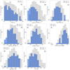 |
Fig. 6. Same as Fig. 5, but for 1.00 < z ≤ 2.45. |
| In the text | |
|
Fig. 7. CDF shown as a function of the size of RLQs. We observe a trend of decreasing CDF as the size of the source increases, possibly showing the effect of Doppler boosting. |
| In the text | |
|
Fig. 8. Box plots as described in Sect. 5.2, which show distributions of black hole mass (left) and Eddington ratio (right) for GRGs, SRGs, SRQs, and GRQs. The number shown in the green box represents the number of sources in each sample. The solid red line indicates the median of the distribution, and the dashed purple line denotes the mean. |
| In the text | |
|
Fig. 9. Correlations between Lbol and QJet in sub-figure (a), Lbol and Pcore in sub-figure (b), and λEdd and Eddington scaled Pcore in sub-figure (c) for GRQs and SRQs. The Spearman’s correlation coefficients are 0.55, 0.65, and 0.70, respectively. |
| In the text | |
Current usage metrics show cumulative count of Article Views (full-text article views including HTML views, PDF and ePub downloads, according to the available data) and Abstracts Views on Vision4Press platform.
Data correspond to usage on the plateform after 2015. The current usage metrics is available 48-96 hours after online publication and is updated daily on week days.
Initial download of the metrics may take a while.