© ESO 2022

1. Introduction

The interpretation of observed radiation emerging, for instance, from galaxies, individual stars, or planetary systems, is key to understanding fundamental properties of the Universe. Deep insight into the underlying physics of an observed object can be obtained by analysing the electromagnetic spectrum of the emitting object. Decoding the information stored within a spectrum, however, is not a simple task. Deducing the fundamental parameters of a single star (i.e. L_*, T_eff, R_*), for example, requires detailed modelling of the stellar atmosphere, possibly relaxing the assumption of local thermal equilibrium (LTE) and accounting for wind outflows. For a given model atmosphere, synthetic spectra then need to be calculated and compared with the observations. In the OB-star regime (on which this paper focusses), state-of-the-art atmospheric modelling and spectral synthesis codes typically assume spherical symmetry (e.g., PHOENIX: Hauschildt 1992; CMFGEN: Hillier & Miller 1998, Hillier 2012; WM-BASIC: Pauldrach et al. 2001; PoWR (see also Sander et al. 2019, Sect. 1): Hamann & Gräfener 2003, Sander et al. 2017; FASTWIND: Sundqvist & Puls 2018, Puls et al. 2020).

Many stars, however, can deviate from spherical symmetry, with perturbations typically induced by magnetic fields, surface (and wind) distortions from rotation, surrounding discs, and binarity or multiplicity effects. Due to the complexity of including full non-LTE occupation numbers within multi-D calculations, corresponding spectral synthesis codes are only gradually developed by applying different solution methods from finite-volume methods (FVM) to short- and long-characteristics methods (SC and LC) to Monte-Carlo methods (MC). A non-exhaustive list of 3D radiative transfer codes accounting for supersonic velocity fields includes Wind3D (see also Lobel & Blomme 2008, Sect. 1; FVM), a code developed by Hennicker et al. (2020) (SC), PHOENIX/3D (Hauschildt & Baron 2006 and other papers in this series, LC), and HDUST (Carciofi & Bjorkman 2006, MC), where the first two examples currently apply a two-level-atom (TLA) approach, whereas the last two include a multi-level description of an atom (of typically one particular species). When the atomic level populations are obtained by such codes, the synthetic spectra can be calculated by solving the equation of radiative transfer along the direction to the observer, for instance, by applying the LC method in a cylindrical coordinate system based on Lamers et al. (1987), Busche & Hillier (2005), Sundqvist et al. (2012), see also Hennicker et al. (2018).

Thus far, the above described codes and methods have been tailored to the spectral synthesis of single stars in 1D or 3D. To our knowledge, there exists no viable multi-D alternative to calculating synthetic spectra from massive-star binary systems with circumstellar material around them. For example, the SPAMMS-code by Abdul-Masih et al. (2020b) relies on patching the emergent intensities as obtained from several 1D spherically symmetric FASTWIND models. Thus, the effect of rays propagating through the winds of both individual stars is neglected. Moreover, such models cannot be used for arbitrary 3D structures such as circumstellar discs.

In this paper, we thus develop a general purpose spectral synthesis tool for binary systems (BOSS-3D, i.e. binary-object spectral-synthesis in 3D)¹ by extending the solution method for single stars from Hennicker et al. (2018) using simple coordinate transformations. For given atmospheric and circumstellar structure(s) with (thus far approximate) occupation numbers, this code accounts for large-scale, possibly structured outflows or discs within both involved systems, thus circumventing the aforementioned shortcomings of previous methods. By allowing for different length scales of the involved objects, the code can also be used to analyse transit spectra of planetary systems. The basic idea of our method relies on defining two (independent) coordinate systems for the individual objects, and applying the standard single-star pz-geometry to each of the systems. To correctly account for overlapping coordinates (e.g., during transits), the individual systems are merged by triangulation.

As a first application of the newly developed algorithm, we considered the binary (or multiple) system LB-1. The spectrum of this system clearly shows an anti-phase behaviour of stellar absorption lines against the line wings of a broad H_α emission (Liu et al. 2019). Yet the interpretation of these findings is still under debate. Based on these observations and the corresponding orbital reconstruction, Liu et al. (2019) proposed a binary system with period P ≈ 79 d, consisting of a B star (visible component) and a 70 M_⊙ black hole (BH) with associated disc yielding the H_α emission. Since it is difficult to explain the origin of a 70 M_⊙ BH in the Milky Way from stellar evolution theory (though, see Belczynski et al. 2020), there has been vivid discussion about LB-1 in the literature. While Simón-Díaz et al. (2020) re-analysed the visible component (B star, primary object) and found a significantly lower mass for the B star thus also reducing the BH mass, Abdul-Masih et al. (2020a) and El-Badry & Quataert (2020) showed that the wobbling H_α wings could also be explained by a superposed broad H_α absorption component on a static emission profile, thus questioning the BH hypothesis as a whole. Shenar et al. (2020) disentangled the optical spectra of LB-1 and proposed a binary system consisting of a stripped He-star (the primary) in a 79 d orbit with a rapidly-rotating Be-star, presumably the product of a recent mass-transfer event. Alternatively, Rivinius et al. (2020) proposed that the Be-star is a tertiary object, leaving the secondary component unidentified. Recently, Lennon et al. (2021) modelled the spectral energy distribution (SED) of LB-1 in the optical and ultra-violet regime using 1D plane-parallel model-atmospheres, and compared several models (including the aforementioned stripped-star/Be-star and B-star/BH hypotheses) with observations from the Hubble Space Telescope. While their models slightly favour the B-star and BH scenario, the stripped-star and Be-star hypothesis could not be ruled out entirely. Throughout this paper, these two competing scenarios will be abbreviated by the B+BH and the strB+Be scenario, respectively.

In this paper, we aim to provide further constraints on LB-1 by applying the BOSS-3D code to models that represent the main hypotheses detailed above, namely the B+BH and the strB+Be binary scenarios. By calculating the corresponding H_α line profiles, we show that both hypotheses can explain the observed phase-dependent H_α line profile provided the LB-1 system contains an additional disc attached to the B-star primary (i.e. either to the B star in the B+BH scenario, or to the stripped star in the strB+Be scenario). The paper is structured as follows. In Sect. 2 we review the basic numerical techniques for spectral synthesis of single objects, in Sect. 3 we extend these methods to binary systems, and in Sect. 4 we apply the developed code to the LB-1 system. Finally, we summarize our findings in Sect. 5.

2. Single-star spectral synthesis

In this section, we briefly summarize the basic solution method for obtaining synthetic spectra from a given single-star model in 3D. Following, for instance, Busche & Hillier (2005), the radiation flux at frequency ν emerging from any unresolved emitting object as seen by an observer at distance d can be formulated as

$$\begin{array}{c}\hfill F_{\nu }={\displaystyle \frac{1}{d^2}}{\displaystyle {\int }_0^{2\pi }{\int }_0^{R_{\max }}{I}_{\nu }(p,\zeta ,\stackrel{\sim }{z}=R_{\max })p\mathrm{d}p\mathrm{d}\zeta ,}\end{array}$$(1)

where R_max is the maximum size of the emitting object, (p,ζ) are polar coordinates describing the projected disc of the emitting object perpendicular to the observer’s direction n, and I_ν is the emergent specific intensity into that direction evaluated at a distance $\stackrel{\sim }{z}=R_{\max }$.

The flux can then be obtained by numerically integrating the emergent specific intensity over the projected disc, with the intensity to be calculated by solving the equation of radiative transfer along all rays in the discretized (p_i, ζ_j) domain of a cylindrical coordinate system ${\mathrm{\Sigma }}_{\mathrm{cyc}}^{(\mathrm{ray})}=(p,\zeta ,\stackrel{\sim }{z})$ with corresponding Cartesian reference frame ${\mathrm{\Sigma }}_{\mathrm{cac}}^{(\mathrm{ray})}=(\stackrel{\sim }{x},\stackrel{\sim }{\mathit{y}},\stackrel{\sim }{z})$, and with the $\stackrel{\sim }{z}$-axis being aligned with the direction to the observer (see also Fig. 1). The corresponding (time-independent) equation of radiative transfer reads:

$$\begin{array}{c}\hfill {\displaystyle \frac{\mathrm{d}{I}_{\nu }(p_i,{\zeta }_j,\stackrel{\sim }{z})}{\mathrm{d}\stackrel{\sim }{z}}}={\chi }_{\nu }(p_i,{\zeta }_j,\stackrel{\sim }{z})[S_{\nu }(p_i,{\zeta }_j,\stackrel{\sim }{z})-I_{\nu }(p_i,{\zeta }_j,\stackrel{\sim }{z})],\end{array}$$(2)

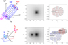Fig. 1. Geometry used for the single-star algorithm (top panels) and for the binary code (bottom panels). Top left panel: cylindrical coordinate system ${\mathrm{\Sigma }}_{\mathrm{cyc}}^{(\mathrm{ray})}$ (blue) with corresponding Cartesian reference frame ${\mathrm{\Sigma }}_{\mathrm{cac}}^{(\mathrm{ray})}$ (red) for an observer’s direction $\mathit{n}\Vert {\mathit{e}}_{\stackrel{\sim }{z}}$ used to obtain the synthetic spectrum of a given (single) object described in a spherical coordinate system ${\mathrm{\Sigma }}_{\mathrm{spc}}^{(\mathrm{obj})}$ (magenta) with corresponding Cartesian reference frame ${\mathrm{\Sigma }}_{\mathrm{cac}}^{(\mathrm{obj})}$ (black). Top middle panel: p − ζ (or $\stackrel{\sim }{x}-\stackrel{\sim }{\mathit{y}}$-plane) of the cylindrical coordinate system (perpendicular to the observer’s direction). Top right panel: an arbitrary $p-\stackrel{\sim }{z}$-slice, with ${\mathit{e}}_{\stackrel{\sim }{z}}$ pointing towards the observer. The grey circles indicate the radial grid of the spherical coordinate system of a considered (single) object, and the black arrows correspond to the individual rays for each impact parameter p. The radiative transfer is then performed along each ray with corresponding discretized ${\stackrel{\sim }{z}}_k$ coordinates indicated by the red dots. Bottom left panel: two local coordinate systems Σ1 and Σ2 describing two individual objects indicated by the cyan and magenta quarter-circles, respectively. Both coordinate systems are embedded within a global coordinate system Σ0 (typically but not necessarily chosen to be the centre of mass of both objects). The vectors t1 and t2 describe the origin of the local coordinate systems in the global coordinate system. Bottom middle panel: as top middle panel, however showing the triangulation of the $\stackrel{\sim }{x}-\stackrel{\sim }{\mathit{y}}$-plane for an arbitrary orbital configuration in a global cylindrical coordinate system within the binary algorithm. Bottom right panel: as top right panel, but now for the binary system. The individual $\stackrel{\sim }{z}$-rays propagating through the system of object 1 (blue) and object 2 (red) potentially need to be merged.

with the opacity χ_ν and source function S_ν describing the absorption and emission of all continuum and line processes. For simplicity, we neglect continuum processes in the following and only consider a single line transition between lower and upper level l ↔ u with transition frequency ν_lu. Further, we omit the notation for explicit spatial dependencies. Then, the opacity and source functions are given by:

$$\begin{array}{cc}& {\chi }_{\nu }={\displaystyle \frac{\pi {\mathrm{e}}^2}{m_{e}c}}\left(gf\right)[{\displaystyle \frac{n_l}{g_l}}-{\displaystyle \frac{n_u}{g_u}}]{\mathrm{\Phi }}_{\mathit{lu}}\left(\nu \right)\hfill \end{array}$$(3)

$$\begin{array}{cc}\hfill & S_{\nu }={\displaystyle \frac{2h{\nu }_{\mathit{lu}}^3}{c^2}}{\displaystyle \frac{1}{{\displaystyle \frac{n_l}{n_u}}{\displaystyle \frac{g_l}{g_u}}-1}},\hfill \end{array}$$(4)

where n_l and n_u are the occupation numbers, g_l and g_u are the statistical weights, and

$$\begin{array}{c}\hfill {\mathrm{\Phi }}_{\mathit{lu}}\left(\nu \right)={\displaystyle \frac{1}{\sqrt{\pi }\mathrm{\Delta }{\nu }_{\mathrm{D}}}}exp[-{({\displaystyle \frac{\nu -{\nu }_{\mathit{lu}}}{\mathrm{\Delta }{\nu }_{\mathrm{D}}}}-{\displaystyle \frac{\mathit{n}·\mathit{v}}{v_{\mathrm{th}}}})}^2]\end{array}$$(5)

is the profile function (approximated here by a Doppler profile) at observers frame frequency ν including non-relativistic Doppler shifts from the observer’s to the comoving frame via the projected velocity n ⋅ v. The width of the profile, $\mathrm{\Delta }{\nu }_{\mathrm{D}}={\nu }_{\mathit{lu}}{\displaystyle \frac{v_{\mathrm{th}}}{c}}$, is given from the thermal velocity of the considered species with mass number m_A, accounting for the local temperature T and a micro-turbulent velocity v_micro:

$$\begin{array}{c}\hfill v_{\mathrm{th}}=\sqrt{{\displaystyle \frac{2k_{\mathrm{B}}T}{m_{\mathrm{A}}}}+v_{\mathrm{micro}}^2}.\end{array}$$(6)

For a given atmospheric model (with known temperatures, velocity vectors, occupation numbers, and micro-turbulent velocities), the equation of radiative transfer, Eq. (2), becomes an ordinary differential equation with exact solution from any point ${\stackrel{\sim }{z}}_{k-1}$ to ${\stackrel{\sim }{z}}_k$

$$\begin{array}{c}\hfill I_{\nu }\left({\stackrel{\sim }{z}}_k\right)=I_{\nu }\left({\stackrel{\sim }{z}}_{k-1}\right)e^{-\mathrm{\Delta }{\tau }_k}+e^{-\mathrm{\Delta }{\tau }_k}{\displaystyle {\int }_0^{\mathrm{\Delta }{\tau }_k}{e}^{t}S(t)\mathrm{d}t.}\end{array}$$(7)

We note that $\mathrm{\Delta }{\tau }_k:={\int }_{{\stackrel{\sim }{z}}_{k-1}}^{{\stackrel{\sim }{z}}_k}{\chi }_{\nu }\mathrm{d}\stackrel{\sim }{z}$ is the optical-depth increment between two positions along a particular ray. Equation (7) is discretized by approximating the source function by a constant, linear, or quadratic form in optical-depth space (e.g., Hennicker et al. 2020, Eq. (12)) based on Kunasz & Auer (1988, linear and quadratic interpolations) and Hayek et al. (2010, monotonic Bézier interpolations).

Since we expect the input model to be given in spherical coordinates ${\mathrm{\Sigma }}_{\mathrm{spc}}^{(\mathrm{obj})}=(r,\mathrm{\Theta },\mathrm{\Phi })$ with corresponding Cartesian reference frame ${\mathrm{\Sigma }}_{\mathrm{cac}}^{(\mathrm{obj})}=(x,\mathit{y},z)$, and if we assume that all structures are well resolved by the corresponding discretized grid, the discretization of ${\stackrel{\sim }{z}}_k$ is easily constructed following the standard pz-geometry approach (e.g., Mihalas 1978, see also Fig. 1):

$$\begin{array}{c}\hfill {\stackrel{\sim }{z}}_k\in \{\begin{array}{c}[-\sqrt{r_q^2-p_i^2},\sqrt{r_q^2-p_i^2}]\forall r_q\ge |p_i|\mathrm{and}{r}_q\ge R_{\ast },\hfill \\ [\sqrt{R_{\ast }^2-p_i^2},\sqrt{r_q^2-p_i^2}]\forall r_q\ge |p_i|\mathrm{and}{r}_q<R_{\ast },\hfill \end{array}\end{array}$$(8)

where r_q refers to the discretized grid of the spherical coordinate system. Thus, the required coordinates for each ray corresponding to a certain (p_i, ζ_j) pair are determined in the cylindrical coordinate system ${\mathrm{\Sigma }}_{\mathrm{cyc}}^{(\mathrm{ray})}$. All quantities describing the state of the gas along a ray need to be interpolated from the spherical grid of the input model. To this end, we need to transform coordinates from ${\mathrm{\Sigma }}_{\mathrm{cyc}}^{(\mathrm{ray})}\to {\mathrm{\Sigma }}_{\mathrm{cac}}^{(\mathrm{ray})}\to {\mathrm{\Sigma }}_{\mathrm{cac}}^{(\mathrm{obj})}\to {\mathrm{\Sigma }}_{\mathrm{spc}}^{(\mathrm{obj})}$:

$$\left(\begin{array}{c}\tilde{x}\\ \tilde{y}\\ \tilde{z}\end{array}\right)=\left(\begin{array}{c}p\cos \zeta \\ p\sin \zeta \\ \tilde{z}\end{array}\right)$$(9)

$$\begin{array}{cc}\hfill & \left(\begin{array}{c}x\\ y\\ z\end{array}\right)=\left(\begin{array}{ccc}{\mathit{e}}_{\stackrel{\sim }{x}}·{\mathit{e}}_x& {\mathit{e}}_{\stackrel{\sim }{y}}·{\mathit{e}}_x& {\mathit{e}}_{\stackrel{\sim }{z}}·{\mathit{e}}_x\\ {\mathit{e}}_{\stackrel{\sim }{x}}·{\mathit{e}}_y& {\mathit{e}}_{\stackrel{\sim }{y}}·{\mathit{e}}_y& {\mathit{e}}_{\stackrel{\sim }{z}}·{\mathit{e}}_y\\ {\mathit{e}}_{\stackrel{\sim }{x}}·{\mathit{e}}_z& {\mathit{e}}_{\stackrel{\sim }{y}}·{\mathit{e}}_z& {\mathit{e}}_{\stackrel{\sim }{z}}·{\mathit{e}}_z\end{array}\right)·\left(\begin{array}{c}\stackrel{\sim }{x}\\ \stackrel{\sim }{y}\\ \stackrel{\sim }{z}\end{array}\right)=\mathit{A}·\stackrel{\sim }{\mathit{r}}\hfill \end{array}$$(10)

$$\begin{array}{cc}\hfill & \left(\begin{array}{c}r\\ \mathrm{\Theta }\\ \mathrm{\Phi }\end{array}\right)=\left(\begin{array}{c}\sqrt{x^2+y^2+z^2}\\ {tan}^{-1}(\sqrt{x^2+y^2}/z)\\ {tan}^{-1}(y/x)\end{array}\right),\hfill \end{array}$$(11)

with e_x, y, z and ${\mathit{e}}_{\stackrel{\sim }{x},\stackrel{\sim }{\mathit{y}},\stackrel{\sim }{z}}$ the unit vectors of the Cartesian reference frames for the spherical and cylindrical systems, respectively, and A the transformation matrix from the Cartesian ray system to the object’s Cartesian reference frame. The unit vectors ${\mathit{e}}_{\stackrel{\sim }{x}}$ and ${\mathit{e}}_{\stackrel{\sim }{\mathit{y}}}$ can be chosen arbitrarily under the constraint that ${\mathit{e}}_{\stackrel{\sim }{z}}\Vert \mathit{n}$ and ${\mathit{e}}_{\stackrel{\sim }{x}}\perp {\mathit{e}}_{\stackrel{\sim }{\mathit{y}}}\perp {\mathit{e}}_{\stackrel{\sim }{z}}$. With the obtained coordinates in the spherical system of the object, all quantities on the discretized ray are calculated by tri-linear interpolations. To ensure that the line-profile function along a ray is resolved by the $\stackrel{\sim }{z}$-grid, we refine the $\stackrel{\sim }{z}$-grid if the projected velocity steps are above v_th/3.

For a single object, synthetic line profiles are thus obtained for a specific observer’s direction by performing the following steps:

1. Definition of the (p, ζ) grid, and of the transformation matrix relating the Cartesian reference frames of the cylindrical (ray) and spherical (object) coordinate systems.

2. Calculation of the ${\stackrel{\sim }{z}}_k$-grid for each (p_i, ζ_j) following Eq. (8).

3. Transformation of the coordinates $(p_i,{\zeta }_j,{\stackrel{\sim }{z}}_k)$ to the object’s spherical system by Eqs. (9)–(11), and interpolation of all required quantities (i.e. opacities, source functions, and velocity components).

4. Solving the discretized form of the radiative transfer equation, Eq. (7), along each ray to obtain the emerging specific intensity. Boundary conditions are specified by photospheric line profiles for the specific intensity if a ray hits the stellar core (implemented via a user-specified subroutine to couple either line profiles as obtained from Kurucz atmosphere models, e.g., Castelli & Kurucz 2003, or from FASTWIND)². For non-core rays, the incident intensity at the outer boundary is set to zero.

5. Integration of emerging specific intensities over the (p, ζ)-plane by replacing the integral in Eq. (1) with a discretized sum, in order to obtain the flux at a specific frequency bin.

6. Restarting the procedure at step 2 for the next frequency bin.

3. Multi-object spectral synthesis

In this section, we extend the solution scheme for a single object described above to multiple systems by accounting for the appropriate coordinate transformations and triangulation techniques. When accounting for a secondary object, the algorithm above essentially suffers from one key issue, namely the resolution of both involved objects. For instance, the spherical grid of the primary object would not resolve the secondary object in the required detail when simply adding the secondary into the spherical grid. Although a description in Cartesian coordinates (presumably requiring mesh-refinement techniques) might help here, we follow a different path within this paper.

Our method is based on the simple observation that each individual object in a multiple system can be described on an individual spherical grid tailored to the properties (e.g., length scale) of the object (see Fig. 1). All spherical grids are then embedded within a global coordinate system with origin chosen at the centre of mass of the multiple system. To keep track of the coordinate representations for each object q, we define the following transformations between the global system ${\mathrm{\Sigma }}_{\mathrm{cac},0}^{(\mathrm{obj})}$ and the individual systems ${\mathrm{\Sigma }}_{\mathrm{cac},q}^{(\mathrm{obj})}$ (see Appendix A):

$$\begin{array}{cc}& {\mathit{r}}_{\mathrm{cac},0}^{(\mathrm{obj})}={\displaystyle \frac{L_q}{L_0}}{\mathit{Q}}_q·{\mathit{r}}_{\mathrm{cac},q}^{(\mathrm{obj})}+{\mathit{t}}_q\hfill \end{array}$$(12)

$$\begin{array}{cc}\hfill & {\mathit{r}}_{\mathrm{cac},q}^{(\mathrm{obj})}={\displaystyle \frac{L_0}{L_q}}{\mathit{Q}}_q^{-1}·({\mathit{r}}_{\mathrm{cac},0}^{(\mathrm{obj})}-{\mathit{t}}_q),\hfill \end{array}$$(13)

where ${\mathit{r}}_{\mathrm{cac},0}^{(\mathrm{obj})}$ and ${\mathit{r}}_{\mathrm{cac},q}^{(\mathrm{obj})}$ describe the coordinates of a given point in the global and individual systems, respectively, L₀ and L_q are the length scales of the coordinate systems, t_q is the translation vector to the origin of the individual systems measured in the global system, and the transformation matrices Q_q are given by:

$$\begin{array}{c}\hfill {\mathit{Q}}_q=\left(\begin{array}{ccc}{\mathit{e}}_x^{(q)}·{\mathit{e}}_x^{(0)}& {\mathit{e}}_y^{(q)}·{\mathit{e}}_x^{(0)}& {\mathit{e}}_z^{(q)}·{\mathit{e}}_x^{(0)}\\ {\mathit{e}}_x^{(q)}·{\mathit{e}}_y^{(0)}& {\mathit{e}}_y^{(q)}·{\mathit{e}}_y^{(0)}& {\mathit{e}}_z^{(q)}·{\mathit{e}}_y^{(0)}\\ {\mathit{e}}_x^{(q)}·{\mathit{e}}_z^{(0)}& {\mathit{e}}_y^{(q)}·{\mathit{e}}_z^{(0)}& {\mathit{e}}_z^{(q)}·{\mathit{e}}_z^{(0)}\end{array}\right).\end{array}$$(14)

The unit vectors ${\mathit{e}}_{x,\mathit{y},z}^{(q)}$ of the individual coordinate systems ${\mathrm{\Sigma }}_{\mathrm{cac},\mathrm{q}}^{(\mathrm{obj})}$ are described in the global system ${\mathrm{\Sigma }}_{\mathrm{cac},0}^{(\mathrm{obj})}$, and allow for tilts of the individual objects within the global coordinate system. In regions where individual coordinate systems are overlapping, the local state of the gas needs to be described consistently within all grids.

For a given observer’s direction n₀ measured in the global frame then, we compute the corresponding representations in the individual coordinate systems, ${\mathit{n}}_q={\mathit{Q}}_q^{-1}\cdot {\mathit{n}}_0$, and assign cylindrical coordinate systems to each of the objects following the procedure outlined in Sect. 2 by setting ${\mathit{e}}_{\stackrel{\sim }{z}}^{(q)}={\mathit{n}}_q$. Again, to keep track of the different coordinate systems, we define the transformation from the local ray-coordinates to the local object coordinates:

$$\begin{array}{c}\hfill {\mathit{r}}_{\mathrm{cac},q}^{(\mathrm{obj})}={\mathit{A}}_q·{\mathit{r}}_{\mathrm{cac},q}^{(\mathrm{ray})}⟺{\mathit{r}}_{\mathrm{cac},q}^{(\mathrm{ray})}={\mathit{A}}_q^{-1}·{\mathit{r}}_{\mathrm{cac},q}^{(\mathrm{obj})},\end{array}$$(15)

with transformation matrix

$$\begin{array}{c}\hfill {\mathit{A}}_q=\left(\begin{array}{ccc}{\mathit{e}}_{\stackrel{\sim }{x}}^{(\mathrm{q})}·{\mathit{e}}_x& {\mathit{e}}_{\stackrel{\sim }{y}}^{(\mathrm{q})}·{\mathit{e}}_x& {\mathit{e}}_{\stackrel{\sim }{z}}^{(\mathrm{q})}·{\mathit{e}}_x\\ {\mathit{e}}_{\stackrel{\sim }{x}}^{(\mathrm{q})}·{\mathit{e}}_y& {\mathit{e}}_{\stackrel{\sim }{y}}^{(\mathrm{q})}·{\mathit{e}}_y& {\mathit{e}}_{\stackrel{\sim }{z}}^{(\mathrm{q})}·{\mathit{e}}_y\\ {\mathit{e}}_{\stackrel{\sim }{x}}^{(\mathrm{q})}·{\mathit{e}}_z& {\mathit{e}}_{\stackrel{\sim }{y}}^{(\mathrm{q})}·{\mathit{e}}_z& {\mathit{e}}_{\stackrel{\sim }{z}}^{(\mathrm{q})}·{\mathit{e}}_z\end{array}\right),\end{array}$$(16)

and e_x = (1, 0, 0), e_y = (0, 1, 0), e_z = (0, 0, 1) the representation of the object’s local coordinate system within the corresponding basis. Accordingly, we also define a global ‘cylindrical’ coordinate system with ${\mathit{e}}_{\stackrel{\sim }{z}}={\mathit{n}}_0$, since the individual cylindrical coordinate systems may overlap (e.g., during transits). The flux integration, Eq. (1), is then performed in the global cylindrical system, and needs to be adapted to avoid double counting of overlapping areas. To this end, we consider the global 2D Delaunay-triangulation of all (p_i, ζ_j)_q points from all individual cylindrical coordinate systems by using the GEOMPACK2 library³ (Joe 1991). The flux integration, Eq. (1), can then be performed by numerically integrating the intensities over all triangles.

With Eqs. (12), (13), and (15) representing the formalism to transform coordinates between the individual and global ray and object systems, the basic algorithm is then defined as follows:

1. Definition of the individual coordinate systems for all objects q, that is length-scales L_q, translation vectors t_q, basis vectors (described in the global coordinate system) ${\mathit{e}}_{x,\mathit{y},z}^{(\mathrm{q})}$, global velocities v^(q) (corresponding to the orbital velocities of the objects), and calculation of the transformation matrices Q_q via Eq. (14).

2. Definition of the (p, ζ)_q grid for all objects q, and calculation of the transformation matrices between ray and object coordinate systems A_q via Eq. (16).

3. Transformation of all (p, ζ)_q coordinates to the global ray-coordinate system using Eqs. (12) and (15) to obtain the corresponding $(\stackrel{\sim }{x},\stackrel{\sim }{\mathit{y}})$ coordinates in the global ray coordinate system.

4. Calculation of the 2D triangulation in the global ray system.

5. Back-transformation of each $(\stackrel{\sim }{x},\stackrel{\sim }{\mathit{y}})$ coordinate to all individual coordinate systems via Eqs. (13) and (15).

6. Step 2 of the single-star algorithm: Setting the ${\stackrel{\sim }{z}}_q$ grid along a ray within each individual coordinate system following Eq. (8).

7. Step 3 of the single-star algorithm: Transformation of all ${({\stackrel{\sim }{x}}_i,{\stackrel{\sim }{\mathit{y}}}_j,{\stackrel{\sim }{z}}_k)}_q$ coordinates to the individual spherical systems and interpolation of all required physical quantities (i.e. opacities, source functions, velocity fields) onto the ray.

8. Transformation of the individual rays to the global ray system via Eqs. (12) and (15).

9. Merging all individual rays to one single ray for a given $(\stackrel{\sim }{x},\stackrel{\sim }{\mathit{y}})$ point (see Fig. 1).

10. Step 4 of the single-star algorithm: Solving the discretized form of the radiative transfer equation, Eq. (7), along the ray.

11. Step 5 of the single-star algorithm: Integration of emerging specific intensities over the triangulated area in Eq. (1) to obtain the flux at a specific frequency bin.

12. Step 6 of the single-star algorithm: Restarting the procedure at step 6 for the next frequency bin.

With this algorithm, we are able to calculate synthetic line profiles for any given orbital configuration and any given state of the surrounding material. We emphasize that this procedure is independent of the length scales of the individual systems, and automatically accounts for transits. Thus, one could also analyse, for example, planetary atmospheres or complex jet configurations as frequently found in post-asymptotic giant branch binary systems (e.g., Bollen et al. 2020). Moreover, this algorithm can be extended to multiple systems, with the computation time typically scaling linearly with the number of objects, and a quadratic scaling found only for complex situations (e.g., when all involved objects are transiting).

4. LB-1

With the above described algorithm, we can readily tackle binary systems in 3D (see also Appendix B for some test calculations of the code when applied to single-star models). In this section we model the H_α line of the binary (or multiple) system LB-1 as a first application, focussing on the strB+Be scenario by Shenar et al. (2020) and on the original B+BH scenario (though with a revised mass for the B star by Simón-Díaz et al. 2020). For both hypotheses, we adopted the stellar parameters as obtained by these authors. For the B star in the B+BH scenario, Simón-Díaz et al. (2020) applied the 1D spherically symmetric NLTE code FASTWIND to deduce the stellar parameters. Similarly, Shenar et al. (2020) applied the 1D spherically-symmetric NLTE code PoWR (Hamann & Gräfener 2003; Sander et al. 2017) to the disentangled spectrum of the Be-star in the strB+Be scenario, while relying on the Grid Search in Stellar Parameters tool (GSSP, see also Shenar et al. 2020, Appendix B.1; Tkachenko 2015) with synthetic spectra derived from 1D plane-parallel LTE modelling using the SYNTHV (see also Shenar et al. 2020, Appendix B.1) radiative transfer code (Tsymbal 1996) and a grid of LLMODEL (see also Shenar et al. 2020, Appendix B.1) atmospheres (Shulyak et al. 2004) when analysing the stripped star. The updated stellar parameters by Lennon et al. (2021) using the 1D plane-parallel NLTE code TLUSTY (Hubeny 1988, Hubeny & Lanz 1995) are typically in a similar range (see Table 1). These studies relied on investigating photospheric lines that are (at most) very weakly contaminated by the disc (in contrast to H_α, for instance), so that the adopted stellar parameters should be good representatives of the underlying stars. With the given stellar parameters then, we ‘only’ need to define a suitable disc model for the BH disc and the Be-star disc to calculate synthetic H_α line profiles.

To this end, we have set up an axisymmetric analytical model for the disc following Kee et al. (2018) (see also Carciofi & Bjorkman 2006) which is based on a prescribed density stratification in the equatorial plane by a parameterised power-law, and assumes hydrostatic equilibrium in the vertical direction. Then, the density in the disc is:

$$\begin{array}{c}\hfill \rho (r,\mathrm{\Theta })={\rho }_0{\left({\displaystyle \frac{rsin\mathrm{\Theta }}{R_{\ast }}}\right)}^{-{\beta }_{\mathrm{D}}}exp[-{\displaystyle \frac{G{M}_{\ast }}{v_{\mathrm{s}}^2}}({\displaystyle \frac{1}{rsin\mathrm{\Theta }}}-{\displaystyle \frac{1}{r}})],\end{array}$$(17)

with r, Θ the radial and co-latitudinal coordinates, M_* the stellar or BH mass, R_* the stellar radius or the minimum radius of the BH disc, and ρ₀ and β_D the base density and power-law index for the density stratification. When β_D = 15/8, this formulation is equivalent to the standard α-accretion disc model by Shakura & Sunyaev (1973) at large distances from the BH, with the α-prescription and accretion rate hidden⁴ within the parameter ρ_o. As such, ρ₀ is related to the mass flux through the disc, and β_D can be considered as a combined proxy for the disc viscosity, scale height, and temperature as a function of radius (within both a BH accretion or a Be-star decretion disc). For Be-stars, typical values are of the order of β_D ∈ [1.5, 4] and ρ₀ ∈ 5 ⋅ [10⁻¹⁰, 10⁻¹³] g cm⁻³ (based on observations and H_α line fitting, e.g., Silaj et al. 2010, see also the review by Rivinius et al. 2013). With the sound speed, $v_{\mathrm{s}}=\sqrt{k_{\mathrm{B}}T/\mu m_p}$, evaluated here for a typical temperature T = 10 kK and a mean molecular weight μ = 0.6, the disc density is specified for given stellar parameters and the input parameters ρ₀, β_D.

Further, we assumed Keplerian rotation of the disc in the orbital plane of the binary system, with the azimuthal component of the velocity field given as

$$\begin{array}{c}\hfill v_{\mathrm{\Phi }}(r,\mathrm{\Theta })=\sqrt{{\displaystyle \frac{G{M}_{\ast }}{rsin\mathrm{\Theta }}}}.\end{array}$$(18)

Since the temperature stratification crucially depends on the type of the disc (BH-accretion disc or Be-star disc), the formulation corresponding to each individual model will be described in Sects. 4.1 and 4.2, respectively. To calculate H_α opacities and source functions, we applied Eqs. (3) and (4), with occupation numbers calculated from Saha-Boltzmann statistics assuming full ionization.

For such disc models, an overarching goal is to qualitatively reproduce the observed H_α line profiles (see Fig. 2), together with the corresponding dynamical spectrum and the radial velocity curves with a semi-amplitude for the primary and secondary of K₁ ≈ 53 km s⁻¹ and K₂ ≈ [6, 13] km s⁻¹, respectively. For the secondary object, the interpretation of the radial velocity curve crucially depends on the applied method, with essentially two choices at hand. Firstly, the semi-amplitude can be calculated from the barycentric method, where the H_α line centre at each phase is determined by considering the line wings up to a certain flux level. Using this method, Liu et al. (2019) estimated $K_2^{({\text{H}}_{\alpha })}\approx 6\text{km}{\text{s}}^{-1}$. However, as shown by Abdul-Masih et al. (2020a), an absorption component of the primary object could increase the apparent motion of the line wings, thus overestimating the true orbital velocities. Following this argumentation, an emission component of the primary object would underestimate the true orbital velocities when measured with the barycentric method. Alternatively, the orbital solution could be estimated by applying spectral disentangling techniques, with corresponding results expected to represent the actual orbital motion of the objects. Using this method, Shenar et al. (2020) measured $K_2^{(\text{true})}\approx 11\text{km}{\text{s}}^{-1}$ for LB-1, in good agreement with a detailed investigation of near-infrared emission lines by Liu et al. (2020) estimating $K_2^{(\text{true})}\in [8,13]\text{km}{\text{s}}^{-1}$. The differences between the K₂ values as obtained from the barycentric method and the disentangled spectra might then be explained by an emission component attached to the primary object. Our modelling then should ideally reproduce the $K_2^{({\text{H}}_{\alpha })}\approx 6\text{km}{\text{s}}^{-1}$ semi-amplitude when applying the barycentric method to the synthetic H_α lines, while also yielding $K_2^{(\text{true})}\approx 11\text{km}{\text{s}}^{-1}$ from the actual orbit of the system.

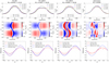Fig. 2. Hα line profiles at different phases φ (top row) with corresponding mean-subtracted dynamical spectra (middle row) and radial velocity curves (bottom row) of the BH or strB companion. The xobs-axis describes the frequency shift from line centre expressed in velocity space. The first three columns to the left display the solution for the three different models, PB_SBH (primary: B star, secondary: BH), PST_SBE01 (primary: stripped star, secondary: Be-star, model 1), PST_SBE02 (primary: stripped star, secondary: Be-star, model 2), with Hα line profiles at two distinct phases from the actual observations indicated by the black dashed and dotted lines. The right column additionally displays the corresponding observed (see Shenar et al. 2020) Hα line profiles, mean-subtracted dynamical spectrum and radial velocity curves of LB-1, where we distinguish between the true ones (e.g., from using disentangling methods) indicated in blue and those obtained from the barycentric method applied to the Hα line wings (red). To reduce the noise, all observed line profiles have been convolved with a Gaussian filter of width 10 km s−1. The bottom panels display the radial velocity curves of the secondary when calculated from the barycentric method applied to the Hα line profile wings (red crosses) and when using the true orbital parameters (blue crosses). Additionally, we display the corresponding radial velocity curves as found by Shenar et al. (2020) and Liu et al. (2019) using disentangling techniques (blue solid line) and the barycentric method (red solid lines), respectively. At the top, the (phase-averaged) equivalent width evaluated in velocity space in units of 100 km s−1 and the inclination used within the synthetic-spectra calculations are indicated.

Since the eccentricity is small (e = 0.03 ± 0.01, see Liu et al. 2019), we assumed a circular orbit. For given masses of the individual objects, M₁, M₂, and an observed orbital period P ≈ 79 d then, the orbit is obtained from the two-body problem:

$$\begin{array}{cc}& a={\left[{\displaystyle \frac{G(M_1+M_2)P^2}{4{\pi }^2}}\right]}^{1/3}\hfill \end{array}$$(19)

$$\begin{array}{cc}\hfill & a_1={\displaystyle \frac{M_2}{M_1+M_2}}a{v}_1={\displaystyle \frac{M_2}{M_1+M_2}}{\displaystyle \frac{2\pi a}{P}}\hfill \end{array}$$(20)

$$\begin{array}{cc}\hfill & a_2={\displaystyle \frac{M_1}{M_1+M_2}}a{v}_2={\displaystyle \frac{M_1}{M_1+M_2}}{\displaystyle \frac{2\pi a}{P}},\hfill \end{array}$$(21)

with a the binary separation, a₁, a₂ the distance of the objects to the centre of mass, and v₁ and v₂ the absolute orbital velocities. Thus, for the observed radial velocity curve(s) and period, and assuming the individual masses of the objects to be given, the inclination i is fixed within our calculations in order to reproduce the semi-amplitude of the radial velocity curve for the primary object by v₁ ⋅ sin(i) = K₁. For our best models, the orbital parameters are summarized in Table 2.

4.1. B-star and BH-disc (B+BH) scenario

In the following, we describe our model for the B+BH scenario (model PB_SBH, primary: B star, secondary: BH). For the B star, we used the stellar parameters as summarized in Table 1. With K₁ and $K_2^{(\text{true})}$ given, the mass of the black hole is constrained via Eqs. (20) and (21) yielding $M_2=M_1{K}_1/K_2^{(\text{true})}\approx [20,30]M_{\odot }$, where we have chosen the black-hole mass as M₂ = 30 M_⊙ and inclination i = 22° in order to reproduce the semi-amplitude of the radial velocity K₁. With this inclination, we adopted a rotational velocity for the B star, $v_{\mathrm{rot}}^{(1)}=21\mathrm{km}{\mathrm{s}}^{-1}$ (with the observed value v sin i = 8 km s⁻¹, Lennon et al. 2021). To model the disc, we have set the minimum radius to $R_{*}^{(2)}=1R_{\odot }$, since any regions with smaller radii would not contribute to the emission due to the small emitting area in any case, and have set the maximum radius of the disc to the distance from the BH to the first Lagrange point.

For a standard α-disc model without irradiation from an external source, we do not expect any emission in H_α, since the surface of the hot regions close to the BH is very small, and the B-star companion completely dominates the total radiation flux. In the B+BH binary system, however, the disc will also be heated by the B-star companion. In order to avoid complex multi-D radiation-hydrodynamic simulations, and to keep our model as simple as possible, we introduced a constant temperature within the disc as a free parameter. With given stellar parameters and inclination then, the model is completely specified by four input parameters, namely the disc temperature, T_disc, the micro-turbulent velocity in the disc, $v_{\mathrm{micro}}^{(2)}$, the base density of the disc, ${\rho }_0^{(2)}$, and the slope of the density stratification, ${\beta }_{\mathrm{D}}^{(2)}$.

We then calculated H_α line profiles with the algorithm described in Sect. 3 for different models (see Appendix C.1). As an inner boundary condition for the specific intensity emerging the B star, we used a photospheric line profile obtained from FASTWIND. Further, we calculated the radial velocity curve from the barycentric method considering only the wings of the H_α lines up to 1/3 of the total height of the H_α line profile as suggested by Liu et al. (2019). The results for our best fit (by eye) with disc temperature, T_disc = 8 kK, micro-turbulent velocity $v_{\mathrm{micro}}^{(2)}=100\mathrm{km}{\mathrm{s}}^{-1}$, base density ${\rho }_0^{(2)}=3\cdot {10}^{-12}\text{g}{\text{cm}}^{-3}$, and radial density stratification β_D = 3/2 are shown in Fig. 2, with corresponding density, temperature, and velocity profiles in the equatorial plane shown in Fig. 3.

Fig. 3. Disc models in the equatorial plane corresponding to our best-fit parameters of the LB-1 system (see Table 3). The top and middle panels display the radial density and temperature stratification, respectively, and the azimuthal velocity component is shown in the bottom panel. The blue and red lines indicate the BH accretion disc (model PBH_SB) and the Be-star disc within the single-disc model (model PST_SBE01), respectively. For model PST_SBE02 (containing two discs), the Be-star disc is indicated by the green dotted line (partially overlapping with the red solid line from model PST_SBE01), and the stripped-star disc is indicated by the green solid line.

The slope of the density stratification is in fairly good agreement with accretion discs described within the α-disc prescription. Indeed, a shallow slope of the density stratification is also required from a modelling point of view to obtain a centrally peaked emission profile. For a steeper decline of the density, for instance, the outer disc regions (where the velocities are lowest) barely contribute to the low-velocity emission due to much smaller densities.

On the other hand, the emitting area at high (projected) velocities (i.e. near to the inner disc radius) is quite small. Thus, a relatively high micro-turbulent velocity is required to obtain the broad H_α emission wings, effectively increasing the emitting area (and consequently the emerging flux) at high velocity shifts. In particular, this also smoothens the typically double-peaked emission feature of accretion discs even at such inclinations (i = 22°). High turbulent velocities, however, are frequently found when modelling dynamical systems with simplified stationary models (which by assumption neglect small-scale turbulent motions in the gas). As just one example, to mimick the observed velocity dispersion when analysing magnetically confined winds described with a steady state model, Owocki et al. (2016) convolved their synthetic H_α line profiles with a 150 km s⁻¹ Gaussian ‘macro-turbulence’ velocity. Since we have neglected gravitational interactions of the primary object with the disc, we might thus expect the inferred high turbulent velocities to mimick dynamical effects within the binary system.

The qualitative behaviour of the observed H_α line profile is well reproduced, with corresponding phase-averaged equivalent width measured in velocity space in units of 100 km s⁻¹, ${\overline{W}}_x=6.81$, in good agreement with observations (${\overline{W}}_x^{(\mathrm{obs})}=6.84$). We emphasize, however, that the radial velocity curves show some discrepancies when compared to observations (see also Table 2). While the actual orbital velocities, $K_2^{(\mathrm{true})}=v_{2}sin\left(i\right)=7.4\mathrm{km}{\mathrm{s}}^{-1}$, are slightly below the observed range ($K_2^{(\mathrm{true},\mathrm{obs})}\in [8,13]\mathrm{km}{\mathrm{s}}^{-1}$), we find a higher semi-amplitude when applying the barycentric method ($K_2^{({\text{H}}_{\alpha })}=10\text{km}{\text{s}}^{-1}$). Indeed, this discrepancy can be explained by the absorption profile of the B star (see discussion in Abdul-Masih et al. 2020a), and could be solved by an additional H_α emission component attached, for example, to the B star or to a tertiary object. Such an additional emission component would reduce the radial velocity amplitude as measured from the barycentric method, by slightly modifying the H_α line wings.

More pronounced, we find significant differences between the observed and synthetic (mean-subtracted) dynamical spectra of the H_α line. While the observed dynamical spectrum clearly displays an anti-phase behaviour of the line wings and the line core, the corresponding features in the synthetic dynamical spectrum are fairly well aligned. As shown below for the strB+Be scenario, this issue could be solved by introducing also a disc around the B star though.

A main theme of our model regards the temperature stratification of the BH disc, where we required T_disc = 8 kK in order to reproduce the observations. This temperature region can indeed be considered as a sweet spot, since lower temperatures (T_disc ≲ 5 kK) would require much higher densities to provide enough emission in H_α. The corresponding densities would translate to a high mass-accretion rate of the BH within the standard α-disc prescription, thus predicting an X-ray bright accretion disc that has not been observed. Similarly, too high temperatures (T_disc ≳ 15 kK) are not allowed either, because we would need to increase the densities to match the equivalent width of the observed H_α line profiles (see Appendix C.1), again yielding an X-ray bright accretion disc. If the sweet-spot temperature as found in our model is a reasonable substitute for detailed numerical simulations still needs to be investigated.

4.2. Stripped-star and Be-star (strB+Be) scenario

For the stellar parameters of the LB-1 system within the strB+Be scenario, we adopted the values proposed by Shenar et al. (2020), summarized again in Table 1, and yielding an inclination i = 39°. Motivated by these authors, we have set the rotational velocity of the stripped star to $v_{\mathrm{rot}}^{(1)}=11$ (with v sin i = 7 km s⁻¹ following Shenar et al. 2020 and Lennon et al. 2021), and assumed the Be-star to rotate at its critical velocity, $v_{\mathrm{rot}}^{(2)}=\sqrt{G{M}_{*}^{(1)}/R_{*}^{(1)}}$. For simplicity, we neglected effects of gravity darkening.

To set the temperature stratification in the disc, we followed the qualitative behaviour as found by detailed radiative-transfer calculations in Carciofi & Bjorkman (2006, Sect. 5.2). In regions close to the stellar surface (where the vertical electron-scattering optical depth τ_z(r sin Θ) > 0.1), we adopted an analytical temperature stratification described by a flat blackbody reprocessing disc (their Eq. (12)):

$$\begin{array}{cc}& T_{\mathrm{disc}}(r,\mathrm{\Theta })={\displaystyle \frac{T_0}{{\pi }^{1/4}}}[{sin}^{-1}\left({\displaystyle \frac{R_{\ast }}{rsin\mathrm{\Theta }}}\right)\hfill \\ \hfill & {-{\displaystyle \frac{R_{\ast }}{rsin\mathrm{\Theta }}}\sqrt{1-{\displaystyle \frac{R_{\ast }^2}{r^2{sin}^2\mathrm{\Theta }}}}]}^{1/4},\hfill \end{array}$$(22)

with T₀ the base temperature of the disc. Since the base densities of our disc models are typically relatively low, we can neglect back-warming effects of the photosphere by the disc, and therefore have set the base temperature to the stellar effective temperature, T₀ = T_eff. To mimick the heating of the disc in (vertically) optically thin regions by the star, we adopted a constant disc temperature T_disc = 0.6 ⋅ T_eff where τ_z(r sin Θ) < 0.1 (again, following the argumentation by Carciofi & Bjorkman 2006).

We note already here that we additionally allowed for a disc attached also to the stripped star (see below). With given stellar parameters, a now specified temperature stratification, and a given inclination to reproduce the semi-amplitude of the radial velocity curve of the primary, K₁, the model is completely specified by six input parameters, namely the micro-turbulent velocities, $v_{\mathrm{micro}}^{(1,2)}$, the base density ${\rho }_0^{(\text{1},\text{2})}$, and the slope of the density stratification of both discs, ${\beta }_{\mathrm{D}}^{(1,2)}$. When considering only the Be-star disc, the number of free parameters is reduced to three.

As for the B+BH scenario above, we calculated synthetic H_α line profiles with the developed BOSS-3D code for various different models (see Appendix C.2), with the photospheric line profiles of both stars again obtained from FASTWIND. The results for our best two models are shown in Fig. 2, with the corresponding density, temperature, and velocity stratification in the equatorial plane shown in Fig. 3, and the orbital and disc parameters summarized in Tables 2 and 3, respectively.

Model PST_SBE01. This model describes a stripped star (primary object) in orbit with a Be-star (secondary object) hosting a circumstellar disc. The obtained disc parameters, ${\beta }_{\mathrm{D}}^{(2)}=3/2$ and ${\rho }_0^{(\text{2})}=6.9\cdot {10}^{-13}\text{g}{\text{cm}}^{-3}$ are both at the lower end of expected values (see above and Silaj et al. 2010), which can be explained as follows: Firstly, the inner regions of the disc (i.e. those near to the star with highest rotational velocities) would become optically thick in the continuum⁵ for higher base densities, and the broad line wings would vanish within the continuum flux. Secondly, as described above for the BH disc, a shallow slope of the density stratification is required to obtain a centrally peaked emission profile. Again, we also require a high micro-turbulent velocity to obtain the broad H_α emission wings and to smooth out the otherwise double-peaked emission profile.

Even for our best fit (by eye) parameters, however, the central emission peak is not well reproduced with this model. Additionally, the equivalent width averaged over all phases (${\overline{W}}_x=6.57$, again measured in 100 km s⁻¹) is somewhat smaller than expected from observations (${\overline{W}}_x^{(\mathrm{obs})}=6.84$). Moreover, the obtained semi-amplitude of the radial velocity of the secondary object, $K_2^{({\text{H}}_{\alpha })}=13\text{km}{\text{s}}^{-1}$, shows a clear deviation from the actually observed values ($K_2^{({\text{H}}_{\alpha },\text{obs})}\approx 6\text{km}{\text{s}}^{-1}$). As in the B+BH scenario, the semi-amplitude is larger than the orbital velocity of the secondary object (v₂sin(i) = 9.9 km s⁻¹), demonstrating again the impact of the photospheric absorption profile underlying the stripped star in this case. Finally, the dynamical H_α line profile shows the same behaviour as for the B+BH scenario, in contrast to observations.

Model PST_SBE02. To improve the model and to increase the low-velocity emission, we additionally implemented a circumstellar disc attached to the stripped star. Although speculative, this disc might have formed by re-accretion from the Be-star (e.g., Shenar et al. 2020) or from earlier mass-transfer phases.

While the best fit (by eye) gives a similar disc for the Be-star as found above, we predict a slightly higher base density of the stripped-star disc, ${\rho }_0^{(\text{1})}=1.3\cdot {10}^{-12}\text{g}{\text{cm}}^{-3}$, and a relatively steep slope of the density stratification, ${\beta }_{\mathrm{D}}^{(1)}=7/2$. Since the orbital velocities of the stripped-star disc are quite low in any case (Eq. (18) with a small mass and large radius), this model gives an increased central emission peak, at least for moderate micro-turbulent velocities. The qualitative behaviour of the observed H_α line profile then is very well reproduced, with corresponding equivalent width, ${\overline{W}}_x^{(\mathrm{obs})}=6.84$, in very good agreement with observations. Since the H_α line wings are slightly contaminated by the (anti-phase) emission from the stripped-star disc, the obtained radial velocity curve ($K_2^{({\text{H}}_{\alpha })}=8\text{km}{\text{s}}^{-1}$) agrees fairly well with the corresponding observations ($K_2^{({\text{H}}_{\alpha },\text{obs})}=6\text{km}{\text{s}}^{-1}$ as derived from the observed H_α line wings). This underestimation of the true orbital velocities due to the contamination of the line profile by an emission component from the primary object is tightly connected to the opposite effect as found by Abdul-Masih et al. (2020a) for an absorption component.

While we were not aiming at an exact reproduction of the radial velocity curves due to the simplicity of our disc model (e.g., neglecting disc inhomogeneities), we show that the disc’s emission component can qualitatively explain the discrepancies between the true and apparent orbital motion of the system. We emphasize that any sort of relatively narrow, centrally peaked H_α emission originating from the stripped star might provide similar results. The origin of such narrow H_α emission, however, remains unclear. For instance, we were not able to reproduce the observations with a simple (β-velocity-type) stellar wind blown from the stripped star. In contrast, the dynamical spectrum of our strB+Be model with an additional disc around the stripped star is in good agreement with observations. Thus, and due to the simplicity of our disc model (with only three free parameters for each disc), we propose that LB-1 contains two discs, each attached to the individual objects in a strB+Be binary system (as shown here), or in a B+BH binary (as qualitatively explained above). We emphasize that Shenar et al. (2020) found a centrally peaked H_α emission from the stripped star by using disentangling techniques as well, suggesting that this residual component might originate from a disc around the stripped star. Our present results put this interpretation on a much firmer ground.

5. Summary and conclusions

In this paper, we have presented a new method for calculating synthetic spectra of binary systems, assuming the orbital setup and the atmospheric and circumstellar structure(s) to be known. This method can be extended to multiple systems, with the computation time scaling only linearly (or slightly super-linearly) with the number of involved objects. Moreover, by assigning individual coordinate systems to each object and accounting for the appropriate coordinate transformations, the developed method automatically accounts for the different length-scales of each object. The presented algorithm and associated code (BOSS-3D) is therefore capable of calculating synthetic line profiles for a wide variety of astrophysical systems, such as planetary or stellar transits, jets associated with young stellar objects (YSO’s) or post-asymptotic giant branch binary systems (see also Bollen et al. 2020), and multiple systems involving (possibly colliding) stellar winds, Be stars, or black holes (BH’s) with discs.

As a first application of the method, we considered the H_α line formation of the B-star/BH-disc (B+BH) and stripped-star/Be-star (strB+Be) scenarios for the enigmatic (multiple) system LB-1 that have previously been proposed (among other hypotheses, see Sect. 1) by Liu et al. (2019) and Shenar et al. (2020), respectively. To calculate the density stratification and velocity field, we applied an analytical, geometrically thin, Keplerian disc model in vertical hydrostatic equilibrium. Further, we assigned a constant temperature to the BH disc as a free parameter, and used a prescribed temperature stratification based on Carciofi & Bjorkman (2006) for the Be-star disc. The level populations for the H_α line transition have then been computed from Saha-Boltzmann statistics assuming full ionization.

Under these assumptions none of the models can reproduce the detailed phase-dependent shape of the observed line profiles, particularly due to differences in the dynamical spectrum (and missing low-velocity emission in some cases). Moreover, the radial velocity curves measured from the synthetic H_α line wings are highly overestimated due to the absorption component of the primary object (see also Abdul-Masih et al. 2020a). It remains open whether NLTE calculations can help to explain the detailed phase-dependent shape of H_α line profiles. Detailed theoretical investigations are needed to test these effects. Alternatively, we have empirically set an additional disc around the stripped star within the strB+Be scenario to solve this problem, and found a sound reproduction of the observed H_α line profiles both from their qualitative shape and their equivalent widths, as well as of the dynamical spectrum and the radial velocity curves. This putative disc might be a remnant associated with earlier mass-transfer phases or could have originated from re-accretion of material from the Be-star disc.

Similarly, such a disc might be attached to the B star in the B+BH scenario as well, and the B+BH hypothesis remains a valid possibility to explain the LB-1 system. In any case, our findings provide strong evidence that LB-1 contains a disc-disc system, with an additional disc either attached to the B star (in the B+BH scenario) or to the stripped star (in the strB+Be scenario).

Acknowledgments

We thank our referee, Dr. Maria Bergemann, for many helpful comments and suggestions. L. H. and J. O. S. gratefully acknowledge support from the Odysseus program of the Belgian Research Foundation Flanders (FWO) under grant G0H9218N. J. B. acknowledges support from the FWO Odysseus program under project G0F8H6N. The National Solar Observatory (NSO) is operated by the Association of Universities for Research in Astronomy, Inc. (AURA), under cooperative agreement with the National Science Foundation. T.S. acknowledges funding received from the European Research Council (ERC) under the European Union’s Horizon 2020 research and innovation programme (grant agreement number 772225: MULTIPLES) and from the European Union’s Horizon 2020 under the Marie Skłodowska-Curie grant agreement No 101024605. I.E.M. has received funding from the European Research Council (ERC) under the European Union’s Horizon 2020 research and innovation programme (SPAWN ERC, grant agreement No 863412).

References

Appendix A: Coordinate transformations

In this section, we derive the basic transformations of coordinates between two coordinate systems (see Fig. A.1) with orthogonal basis such that ${\mathrm{\Sigma }}_1=\left({\mathit{e}}_x^{(1)},{\mathit{e}}_y^{(1)},{\mathit{e}}_z^{(1)}\right)$ and ${\mathrm{\Sigma }}_2=\left({\mathit{e}}_x^{(2)},{\mathit{e}}_y^{(2)},{\mathit{e}}_z^{(2)}\right)$. Any point r_Σ1 in Σ₁ can then be expressed by

$$\begin{array}{cc}\hfill {\mathit{r}}_{{\mathrm{\Sigma }}_1}& =x_1{\mathit{e}}_x^{(1)}+y_1{\mathit{e}}_y^{(1)}+z_1{\mathit{e}}_z^{(1)}\hfill \\ \hfill & =s_x{x}_2{\mathit{e}}_x^{(2)}+s_y{y}_2{\mathit{e}}_y^{(2)}+s_z{z}_2{\mathit{e}}_z^{(2)}+\mathit{t},\hfill \end{array}$$(A.1)

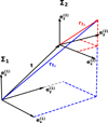Fig. A.1. Transformation between coordinate systems ${\mathrm{\Sigma }}_1=\left({\mathit{e}}_x^{(1)},{\mathit{e}}_y^{(1)},{\mathit{e}}_z^{(1)}\right)$ and ${\mathrm{\Sigma }}_2=\left({\mathit{e}}_x^{(2)},{\mathit{e}}_y^{(2)},{\mathit{e}}_z^{(2)}\right)$, where t indicates the translation vector from Σ1 → Σ2, and rΣ1 and rΣ2 denote the coordinate representations in each system for a given point.

where (x₁, y₁, z₁) and (x₂, y₂, z₂) are the coordinates in each system, s_x, y, z are scale factors allowing us to include different length scales for both coordinate systems, $\mathit{t}=t_x{\mathit{e}}_x^{(1)}+t_y{\mathit{e}}_y^{(1)}+t_z{\mathit{e}}_z^{(1)}$ is the translation vector indicating the origin of Σ₂ within Σ₁, and ${\mathit{e}}_{x,y,z}^{(2)}$ are the basis vectors of Σ₂ measured within Σ₁.

For our purposes, the length scales of both coordinate systems are constant (and typically refer to the radius of each individual object). Thus, we define s := L_Σ2/L_Σ1 = s_x = s_y = s_z, with L_Σ2 and L_Σ1 describing the length scales of the individual coordinate systems. Multiplying Eq. (A.1) with ${\mathit{e}}_x^{(1)}$, ${\mathit{e}}_y^{(1)}$, and ${\mathit{e}}_z^{(1)}$, we obtain in matrix form:

$$\begin{array}{cc}\hfill \underset{{\mathit{r}}_{{\mathrm{\Sigma }}_1}}{\underbrace{\left(\begin{array}{c}{x}_1\\ y_1\\ z_1\end{array}\right)}}& =\underset{=:\mathit{S}}{\underbrace{\left(\begin{array}{ccc}s& 0& 0\\ 0& s& 0\\ 0& 0& s\end{array}\right)}}\underset{=:\mathit{A}}{\underbrace{\left(\begin{array}{ccc}{\mathit{e}}_x^{(2)}·{\mathit{e}}_x^{(1)}& {\mathit{e}}_y^{(2)}·{\mathit{e}}_x^{(1)}& {\mathit{e}}_z^{(2)}·{\mathit{e}}_x^{(1)}\\ {\mathit{e}}_x^{(2)}·{\mathit{e}}_y^{(1)}& {\mathit{e}}_y^{(2)}·{\mathit{e}}_y^{(1)}& {\mathit{e}}_z^{(2)}·{\mathit{e}}_y^{(1)}\\ {\mathit{e}}_x^{(2)}·{\mathit{e}}_z^{(1)}& {\mathit{e}}_y^{(2)}·{\mathit{e}}_z^{(1)}& {\mathit{e}}_z^{(2)}·{\mathit{e}}_z^{(1)}\end{array}\right)}}\underset{{\mathit{r}}_{{\mathrm{\Sigma }}_2}}{\underbrace{\left(\begin{array}{c}{x}_2\\ y_2\\ z_2\end{array}\right)}}\hfill \\ \hfill & +\underset{\mathit{t}}{\underbrace{\left(\begin{array}{c}{t}_x\\ t_y\\ t_z\end{array}\right)}}.\hfill \end{array}$$(A.2)

Thus, the transformations between the coordinate systems Σ₁ ↔ Σ₂ are readily given by:

$$\begin{array}{cc}\hfill {\mathit{r}}_{{\mathrm{\Sigma }}_1}& =\left[\mathit{S}\mathit{A}\right]·{\mathit{r}}_{{\mathrm{\Sigma }}_2}+\mathit{t}\hfill \end{array}$$(A.3)

$$\begin{array}{cc}\hfill {\mathit{r}}_{{\mathrm{\Sigma }}_2}& ={\left[\mathit{S}\mathit{A}\right]}^{-1}·[{\mathit{r}}_{{\mathrm{\Sigma }}_1}-\mathit{t}].\hfill \end{array}$$(A.4)

Appendix B: Test calculations

In this section, we test the developed BOSS-3D code by calculating synthetic line profiles of a generic resonance-line transition within a spherically symmetric wind of a prototypical hot, massive star. In order to compare the results with the single-object code described in Sect. 2, the secondary object is assumed to be dark ($T_{\mathrm{eff}}^{(2)}=10\mathrm{K}$) and small ($R_{*}^{(2)}=0.2R_{\odot }$). The coordinate system of the secondary object, however, has been set to a large extent, in order to test if the routines for setting up the triangulation and the individual rays are performing reasonably well. By assigning an artificial circular orbit with absolute velocity v_orb = 1000 km s⁻¹ to the primary object, we further test if the corresponding Doppler-shifts are correctly implemented for different viewing angles. The primary object is described by $R_{*}^{(1)}=20R_{\odot }$, $T_{\mathrm{eff}}^{(1)}=40\mathrm{kK}$, and with a wind stratification given from a β-velocity law with base velocity v_min = 10 km s⁻¹, terminal velocity v_∞ = 2000 km s⁻¹, and β = 1. The required density is obtained from the continuity equation assuming a mass-loss rate Ṁ = 10⁻⁶ M_⊙ yr⁻¹, and the source function is calculated from the Sobolev approximation (Sobolev 1960) for a pure scattering line within the two-level approach. Finally, we specify the boundary condition by the Planck function, $I_{\nu }=B_{\nu }(T_{\mathrm{eff}}^{(1,2)})$ , if a ray hits the core of one of the objects.

Figure B.1 displays the resulting line profiles for edge-on observer directions at different phases, compared with the result from the single-object code. Since the relative error remains below few percent, we are highly confident that the algorithm also works for more complex simulations. Moreover, the expected velocity shift at the different phases is exactly reproduced. We finally emphasize that we obtain the same results when interchanging the primary and secondary object within our algorithm, as required.

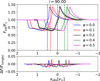Fig. B.1. Top panel: Synthetic line profiles as a function of frequency shift from line centre in units of the terminal velocity for our spherically symmetric test model (see text). The solid lines indicate the line profiles as obtained from the binary code at different phases φ and a fixed inclination i = 90°, and the grey crosses correspond to the solution as obtained from the single-star code. The vertical dashed lines indicate the transition frequency of the line at the different phases for the assumed orbital configuration. Bottom panel: Relative error of the obtained line profiles at different phases when compared to the single-star code (shifted by the corresponding projected orbital velocities).

Appendix C: Parameter study

In this section, we perform a parameter study of the disc model introduced in Sect. 4, and investigate the main effects of the different model parameters on the various measured quantities (i.e. the line-profile shape, the equivalent width, the radial-velocity curve and its semi-amplitude). To this end, we focus on the B-star and BH-disc scenario (model PB_SBH), and on the stripped-star and Be-star scenario with two discs (model PST_SBE02). The individual disc parameters are varied one at a time, starting from our best-fit by eye models presented in Sect. 4 and summarized in Table 3. The radial-velocity curves have been derived from the H_α line wings defined as those parts of the synthetic line profile with normalized flux below a threshold of 1/3 of the flux peak (see also Liu et al. 2019).

C.1. Parameter study for the B-star and BH-disc scenario

Figure C.1 displays the results of our parameter study for the B-star and BH-disc scenario, with variations of the four free parameters, namely the disc’s base density, ${\rho }_0^{(\text{2})}\in 3\cdot [{10}^{-13},{10}^{-11}]\text{g}{\text{cm}}^{-3}$, the slope of the density stratification, ${\beta }_{\mathrm{D}}^{(2)}\in [1.5,4]$, the disc’s temperature $T_{\mathrm{disc}}^{(2)}\in [6,15]\mathrm{kK}$, and the micro-turbulent velocity, $v_{\mathrm{micro}}^{(2)}\in [15,105]\mathrm{km}{\mathrm{s}}^{-1}$. Additionally, we display the reduced χ²-values of the equivalent width and the radial-velocity semi-amplitude as compared to the observations, as well as the combined reduced χ²-value (with an equal weight to both quantities).

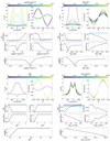Fig. C.1. Parameter study with base parameters defined in Table 3 for model PB_SBH. Upper left main-panel: Synthetic line profiles at phase φ = 0 (top left sub-panel), radial-velocity curve (top right sub-panel), equivalent width with corresponding reduced χ2-value (middle left sub-panels), semi-amplitude of the radial velocity curve with corresponding reduced χ2-value (middle right sub-panels), and total reduced χ2-value (bottom panel), all as a function of the disc’s base density, ${\rho }_0^{(\text{2})}$. The black dotted line indicates our best-fit by eye (see Sect. 4.1), and the blue dashed lines display the observed values with corresponding error-bars (blue-shaded area). Similarly, the top right to bottom right main-panels indicate the dependence of our measurable quantities on the disc’s temperature, $T_{\mathrm{disc}}^{(2)}$, the slope of the density stratification, ${\beta }_{\mathrm{D}}^{(2)}$, and the micro-turbulent velocity, $v_{\mathrm{micro}}^{(2)}$.

Impact of ${\rho }_0^{(\text{2})}$. The strength of the line (and thus also the equivalent width) increases with increasing base density of the disc. Indeed, the equivalent width follows roughly a quadratic dependence, following the ρ²-dependence of the opacity for recombination lines. For low densities, only the photospheric line profile from the primary object (the B star in this scenario) is visible. Thus, the radial velocity curve when measured from the H_α-line wings follows the B-star orbit (K₁ = 53 km s⁻¹) for low base densities, and the BH orbit (K₂ = 7.4 km s⁻¹) for high base densities, as expected. Additionally, the overestimation of the radial-velocity amplitude due to the anti-phase motion of the stellar absorption profile (see Abdul-Masih et al. 2020a) is clearly observed within our models at intermediate densities.

Impact of $T_{\mathrm{disc}}^{(2)}.$ The strength of the H_α line decreases with increasing disc temperature. This effect can be explained as follows. With increasing temperature, the occupation numbers of the lower level become diminished due to the Boltzmann factor. Thus, the opacity is considerably reduced, and the disc essentially becomes transparent in H_α at high temperatures. We emphasize that also at temperatures $T_{\mathrm{disc}}^{(2)}\lesssim 6\mathrm{kK}$ (not shown here), the opacity drops significantly since most hydrogen will be found in the ground state. As before, the radial velocity curve measured from the H_α line follows the BH orbit for low temperatures (and thus a strong disc emission). With increasing disc temperature, the semi-amplitude of the radial velocity curve becomes overestimated when measured from the H_α-line wings due to the anti-phase motion of the stellar absorption profile. In contrast to the low-density regime described above, the H_α-line wings are mainly controlled by the disc emission at the upper temperature limit, and the radial-velocity curve is therefore following the BH orbit for the full parameter space considered here.

Impact of ${\beta }_{\mathrm{D}}^{(2)}.$ With increasing slope of the disc’s density stratification, the H_α-line profile switches rapidly from showing a significant disc emission to the (almost) pure absorption profile from the B star. Clearly, for ${\beta }_{\mathrm{D}}^{(2)}\gtrsim 2$, the disc emission vanishes due to decreased densities (in particular at large distances from the BH and therefore low velocities). The corresponding radial velocity curves are slightly underestimating the true orbital velocity of the B star (K₁ = 53 km s⁻¹) due to a slight emission from the disc in the H_α-line wings (probing the high-velocity regions and thus the inner parts of the disc).

Impact of $v_{\mathrm{micro}}^{(2)}$. Both the strength of the line and the radial velocity curve are only mildly affected by the micro-turbulent velocity in the disc. The shape of the H_α-line profile, however, switches from a relatively narrow and strongly pronounced double-peaked feature at low $v_{\mathrm{micro}}^{(2)}$ to a broad and smooth one at high $v_{\mathrm{micro}}^{(2)}$. When compared to observations (see Sect. 4), the latter is to be preferred.

Investigation of χ². The χ²-values shown in Fig. C.1 indicate that both the slope of the density stratification and the micro-turbulent velocity are relatively well constrained to the best-fit by eye values found in Sect. 4.1. There exists, however, a slight degeneracy in the disc’s base density and temperature. For instance, one might find a similar good model by decreasing both the disc density and the disc temperature at the same time. With such a model, however, the observed anti-phase behaviour of line core and line wings (see Fig. 2) could not be reproduced either. Moreover, at temperatures $T_{\mathrm{disc}}^{(2)}\lesssim 6\mathrm{kK}$ (not shown here) and $T_{\mathrm{disc}}^{(2)}\gtrsim 15\mathrm{kK}$, the disc’s base density would need to be increased to obtain a significant equivalent width, translating then to an X-ray bright disc that has not been observed.

C.2. Parameter study for the stripped-B and Be scenario with two discs

Figure C.2 displays the results of our parameter study for the stripped-B and Be scenario with two discs, where the discs are described by six free parameters in total, namely the base density for each disc, ${\rho }_0^{(\text{1})}\in [{10}^{-14},{10}^{-11}]\text{g}{\text{cm}}^{-3}$ and ${\rho }_0^{(\text{2})}\in 6\cdot [{10}^{-13},{10}^{-11}]\text{g}{\text{cm}}^{-3}$, the slope of the density stratification, ${\beta }_{\mathrm{D}}^{(1)}$ and ${\beta }_{\mathrm{D}}^{(2)}$ (both in a range ∈[1.5, 4]), and the micro-turbulent velocities, $v_{\mathrm{micro}}^{(1)}$, $v_{\mathrm{micro}}^{(2)}$ (both in a range ∈[15, 105] km s⁻¹). As before, we additionally display the reduced χ²-values calculated for the equivalent width, the radial velocity semi-amplitude, and the equally weighted sum of both.

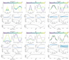Fig. C.2. As Fig. C.1, however for model PST_SBE02 and focussing on the six free parameters ${\rho }_0^{(\text{1})}$, ${\rho }_0^{(\text{2})}$, ${\beta }_{\mathrm{D}}^{(1)}$, ${\beta }_{\mathrm{D}}^{(2)}$, $v_{\mathrm{micro}}^{(1)}$, and $v_{\mathrm{micro}}^{(2)}$.

Impact of ${\rho }_0^{(\text{1})}$ and ${\rho }_0^{(\text{2})}$. The strength of the line increases with increasing base density of the stripped-star disc, ${\rho }_0^{(\text{1})}$, particularly in the low-velocity regions (due to the overall low velocities in the stripped-star disc). At the lower end of our parameter space, the stripped-star disc becomes transparent and the H_α-line profile consists only of three components, namely the absorption profiles of both stars in the binary system, and the disc emission from the secondary object (the Be-star disc). Consequently, the radial-velocity curves vary significantly. For low ${\rho }_0^{(\text{1})}$, the H_α-line wings are probing the Be-star orbit (including the effects of all underlying stellar absorption profiles, of course). With increasing ${\rho }_0^{(\text{1})}$, the radial-velocity amplitude becomes reduced and switches sign at the upper limit of our parameter space due to a significant contamination of the H_α-line emission from the stripped-star disc.

In contrast to the effects of ${\rho }_0^{(\text{1})}$, the strength of the H_α-line profile increases in both the low and high velocity regions with increasing ${\rho }_0^{(\text{2})}$. At the lower end of our parameter space, the line profiles consist only of the emission from the stripped-star disc (and again the stellar absorption components). Thus, the radial velocity curves as obtained from the H_α-line wings follow the stripped-star orbit at low ${\rho }_0^{(\text{2})}$, while the anti-phase behaviour probing the Be-star orbit is measured at high ${\rho }_0^{(\text{2})}$.

Impact of ${\beta }_{\mathrm{D}}^{(1)}$ and ${\beta }_{\mathrm{D}}^{(2)}$. The strength of the H_α-line profile increases with decreasing slope of the stripped-star disc’s density stratification, ${\beta }_{\mathrm{D}}^{(1)}$, in particular in the low-velocity regions. As in Sect. C.1, increasing ${\beta }_{\mathrm{D}}^{(1)}$ translates to decreasing the density of the stripped-star disc, particularly in the outer (low-velocity) regions. Thus, the synthetic line profiles become slightly broader at the upper limit of ${\beta }_{\mathrm{D}}^{(1)}$. Since the stripped-star disc essentially becomes transparent at high ${\beta }_{\mathrm{D}}^{(1)}$, the obtained radial-velocity curve follows the Be-star orbit. Accordingly, the stripped-star orbit is being probed at low ${\beta }_{\mathrm{D}}^{(1)}$, with a significant contamination from the Be-star disc though.

Also with decreasing slope of the Be-star disc’s density stratification, the strength of the H_α-line profile increases, now within both the low and high velocity regions though. At the upper limit of ${\beta }_{\mathrm{D}}^{(2)}$, the Be-star disc becomes transparent and only the stripped-star disc is visible (together with the stellar absorption profiles, again). Thus, a high ${\beta }_{\mathrm{D}}^{(2)}$ is favourable for measuring the stripped-star orbit, while a low ${\beta }_{\mathrm{D}}^{(2)}$ would give the Be-star orbit (still contaminated by the stellar absorption profiles).

Impact of $v_{\mathrm{micro}}^{(1)}$ and $v_{\mathrm{micro}}^{(2)}$. While the equivalent width of the H_α-line profile is only slightly increasing with increasing micro-turbulent velocity of the stripped-star disc ($v_{\mathrm{micro}}^{(1)}$), the shape of the line changes significantly from a double-peaked feature to a relatively smooth and slightly broader appearance. Thus, the radial-velocity curve is probing primarily the Be-star disc at the lower limit of $v_{\mathrm{micro}}^{(1)}$, and the semi-amplitude is increasing with $v_{\mathrm{micro}}^{(1)}$ since the line-profile wings become increasingly contaminated from the stripped-star disc emission.

With increasing micro-turbulent velocity of the Be-star disc ($v_{\mathrm{micro}}^{(2)}$) now, the equivalent width of the H_α-line profile is again only slightly increasing while the shape of the line changes significantly from a relatively narrow double-peaked line profile to a much smoother and broader one. Thus, the radial-velocity curves are probing primarily the Be-star disc at the upper limit of $v_{\mathrm{micro}}^{(2)}$. With decreasing micro-turbulent velocity, the line wings are contaminated by the stripped-star disc, and the semi-amplitude of the radial-velocity curve therefore becomes decreased (towards positive values).

Investigation of χ². As shown by the reduced χ²-values of our stripped-star and Be-star models (Fig C.2), all fit parameters are fairly well constrained to the best-fit by eye values found in Sect. 4.2. There might be a slight degeneracy of the base density and the slope of the density stratification within each of the discs, though. For instance, reducing ${\rho }_0^{(\text{1})}$ and ${\beta }_{\mathrm{D}}^{(1)}$ (or ${\rho }_0^{(\text{2})}$ and ${\beta }_{\mathrm{D}}^{(2)}$) at the same time might give similar results as found for our best-fit model.

All Tables

All Figures

Fig. 1. Geometry used for the single-star algorithm (top panels) and for the binary code (bottom panels). Top left panel: cylindrical coordinate system ${\mathrm{\Sigma }}_{\mathrm{cyc}}^{(\mathrm{ray})}$ (blue) with corresponding Cartesian reference frame ${\mathrm{\Sigma }}_{\mathrm{cac}}^{(\mathrm{ray})}$ (red) for an observer’s direction $\mathit{n}\Vert {\mathit{e}}_{\stackrel{\sim }{z}}$ used to obtain the synthetic spectrum of a given (single) object described in a spherical coordinate system ${\mathrm{\Sigma }}_{\mathrm{spc}}^{(\mathrm{obj})}$ (magenta) with corresponding Cartesian reference frame ${\mathrm{\Sigma }}_{\mathrm{cac}}^{(\mathrm{obj})}$ (black). Top middle panel: p − ζ (or $\stackrel{\sim }{x}-\stackrel{\sim }{\mathit{y}}$-plane) of the cylindrical coordinate system (perpendicular to the observer’s direction). Top right panel: an arbitrary $p-\stackrel{\sim }{z}$-slice, with ${\mathit{e}}_{\stackrel{\sim }{z}}$ pointing towards the observer. The grey circles indicate the radial grid of the spherical coordinate system of a considered (single) object, and the black arrows correspond to the individual rays for each impact parameter p. The radiative transfer is then performed along each ray with corresponding discretized ${\stackrel{\sim }{z}}_k$ coordinates indicated by the red dots. Bottom left panel: two local coordinate systems Σ1 and Σ2 describing two individual objects indicated by the cyan and magenta quarter-circles, respectively. Both coordinate systems are embedded within a global coordinate system Σ0 (typically but not necessarily chosen to be the centre of mass of both objects). The vectors t1 and t2 describe the origin of the local coordinate systems in the global coordinate system. Bottom middle panel: as top middle panel, however showing the triangulation of the $\stackrel{\sim }{x}-\stackrel{\sim }{\mathit{y}}$-plane for an arbitrary orbital configuration in a global cylindrical coordinate system within the binary algorithm. Bottom right panel: as top right panel, but now for the binary system. The individual $\stackrel{\sim }{z}$-rays propagating through the system of object 1 (blue) and object 2 (red) potentially need to be merged.

In the text

Fig. 2. Hα line profiles at different phases φ (top row) with corresponding mean-subtracted dynamical spectra (middle row) and radial velocity curves (bottom row) of the BH or strB companion. The xobs-axis describes the frequency shift from line centre expressed in velocity space. The first three columns to the left display the solution for the three different models, PB_SBH (primary: B star, secondary: BH), PST_SBE01 (primary: stripped star, secondary: Be-star, model 1), PST_SBE02 (primary: stripped star, secondary: Be-star, model 2), with Hα line profiles at two distinct phases from the actual observations indicated by the black dashed and dotted lines. The right column additionally displays the corresponding observed (see Shenar et al. 2020) Hα line profiles, mean-subtracted dynamical spectrum and radial velocity curves of LB-1, where we distinguish between the true ones (e.g., from using disentangling methods) indicated in blue and those obtained from the barycentric method applied to the Hα line wings (red). To reduce the noise, all observed line profiles have been convolved with a Gaussian filter of width 10 km s−1. The bottom panels display the radial velocity curves of the secondary when calculated from the barycentric method applied to the Hα line profile wings (red crosses) and when using the true orbital parameters (blue crosses). Additionally, we display the corresponding radial velocity curves as found by Shenar et al. (2020) and Liu et al. (2019) using disentangling techniques (blue solid line) and the barycentric method (red solid lines), respectively. At the top, the (phase-averaged) equivalent width evaluated in velocity space in units of 100 km s−1 and the inclination used within the synthetic-spectra calculations are indicated.

In the text

Fig. 3. Disc models in the equatorial plane corresponding to our best-fit parameters of the LB-1 system (see Table 3). The top and middle panels display the radial density and temperature stratification, respectively, and the azimuthal velocity component is shown in the bottom panel. The blue and red lines indicate the BH accretion disc (model PBH_SB) and the Be-star disc within the single-disc model (model PST_SBE01), respectively. For model PST_SBE02 (containing two discs), the Be-star disc is indicated by the green dotted line (partially overlapping with the red solid line from model PST_SBE01), and the stripped-star disc is indicated by the green solid line.

In the text

	Fig. A.1. Transformation between coordinate systems ${\mathrm{\Sigma }}_1=\left({\mathit{e}}_x^{(1)},{\mathit{e}}_y^{(1)},{\mathit{e}}_z^{(1)}\right)$ and ${\mathrm{\Sigma }}_2=\left({\mathit{e}}_x^{(2)},{\mathit{e}}_y^{(2)},{\mathit{e}}_z^{(2)}\right)$, where t indicates the translation vector from Σ1 → Σ2, and rΣ1 and rΣ2 denote the coordinate representations in each system for a given point.
In the text

Fig. B.1. Top panel: Synthetic line profiles as a function of frequency shift from line centre in units of the terminal velocity for our spherically symmetric test model (see text). The solid lines indicate the line profiles as obtained from the binary code at different phases φ and a fixed inclination i = 90°, and the grey crosses correspond to the solution as obtained from the single-star code. The vertical dashed lines indicate the transition frequency of the line at the different phases for the assumed orbital configuration. Bottom panel: Relative error of the obtained line profiles at different phases when compared to the single-star code (shifted by the corresponding projected orbital velocities).

In the text

Fig. C.1. Parameter study with base parameters defined in Table 3 for model PB_SBH. Upper left main-panel: Synthetic line profiles at phase φ = 0 (top left sub-panel), radial-velocity curve (top right sub-panel), equivalent width with corresponding reduced χ2-value (middle left sub-panels), semi-amplitude of the radial velocity curve with corresponding reduced χ2-value (middle right sub-panels), and total reduced χ2-value (bottom panel), all as a function of the disc’s base density, ${\rho }_0^{(\text{2})}$. The black dotted line indicates our best-fit by eye (see Sect. 4.1), and the blue dashed lines display the observed values with corresponding error-bars (blue-shaded area). Similarly, the top right to bottom right main-panels indicate the dependence of our measurable quantities on the disc’s temperature, $T_{\mathrm{disc}}^{(2)}$, the slope of the density stratification, ${\beta }_{\mathrm{D}}^{(2)}$, and the micro-turbulent velocity, $v_{\mathrm{micro}}^{(2)}$.

In the text

	Fig. C.2. As Fig. C.1, however for model PST_SBE02 and focussing on the six free parameters ${\rho }_0^{(\text{1})}$, ${\rho }_0^{(\text{2})}$, ${\beta }_{\mathrm{D}}^{(1)}$, ${\beta }_{\mathrm{D}}^{(2)}$, $v_{\mathrm{micro}}^{(1)}$, and $v_{\mathrm{micro}}^{(2)}$.
In the text

References

- Abdul-Masih, M., Sana, H., Conroy, K. E., et al. 2020a, A&A, 636, A59 [NASA ADS] [CrossRef] [EDP Sciences] [Google Scholar]
- Abdul-Masih, M., Banyard, G., Bodensteiner, J., et al. 2020b, Nature, 580, E11 [Google Scholar]
- Belczynski, K., Hirschi, R., Kaiser, E. A., et al. 2020, ApJ, 890, 113 [NASA ADS] [CrossRef] [Google Scholar]
- Bollen, D., Kamath, D., De Marco, O., Van Winckel, H., & Wardle, M. 2020, A&A, 641, A175 [NASA ADS] [CrossRef] [EDP Sciences] [Google Scholar]
- Busche, J. R., & Hillier, D. J. 2005, AJ, 129, 454 [Google Scholar]
- Carciofi, A. C., & Bjorkman, J. E. 2006, ApJ, 639, 1081 [Google Scholar]
- Castelli, F., & Kurucz, R. L. 2003, in Modelling of Stellar Atmospheres, eds. N. Piskunov, W. W. Weiss, & D. F. Gray, 210, A20 [Google Scholar]
- El-Badry, K., & Quataert, E. 2020, MNRAS, 493, L22 [NASA ADS] [CrossRef] [Google Scholar]
- Frank, J., King, A., & Raine, D. J. 2002, Accretion Power in Astrophysics: Third Edition [Google Scholar]
- Hamann, W. R., & Gräfener, G. 2003, A&A, 410, 993 [CrossRef] [EDP Sciences] [Google Scholar]
- Hauschildt, P. H. 1992, J. Quant. Spectr. Rad. Transf., 47, 433 [NASA ADS] [CrossRef] [Google Scholar]
- Hauschildt, P. H., & Baron, E. 2006, A&A, 451, 273 [NASA ADS] [CrossRef] [EDP Sciences] [Google Scholar]
- Hayek, W., Asplund, M., Carlsson, M., et al. 2010, A&A, 517, A49 [NASA ADS] [CrossRef] [EDP Sciences] [Google Scholar]
- Hennicker, L., Puls, J., Kee, N. D., & Sundqvist, J. O. 2018, A&A, 616, A140 [NASA ADS] [CrossRef] [EDP Sciences] [Google Scholar]
- Hennicker, L., Puls, J., Kee, N. D., & Sundqvist, J. O. 2020, A&A, 633, A16 [NASA ADS] [CrossRef] [EDP Sciences] [Google Scholar]
- Hillier, D. J. 2012, in From Interacting Binaries to Exoplanets: Essential Modeling Tools, eds. M. T. Richards, & I. Hubeny, 282, 229 [NASA ADS] [Google Scholar]
- Hillier, D. J., & Miller, D. L. 1998, ApJ, 496, 407 [NASA ADS] [CrossRef] [Google Scholar]
- Hubeny, I. 1988, Comput. Phys. Commun., 52, 103 [Google Scholar]
- Hubeny, I., & Lanz, T. 1995, ApJ, 439, 875 [Google Scholar]
- Joe, B. 1991, Adv. Eng. Software Workstations, 13, 325 [CrossRef] [Google Scholar]
- Kee, N. D., Owocki, S., & Kuiper, R. 2018, MNRAS, 474, 847 [NASA ADS] [CrossRef] [Google Scholar]
- Kunasz, P., & Auer, L. H. 1988, J. Quant. Spectr. Rad. Transf., 39, 67 [NASA ADS] [CrossRef] [Google Scholar]
- Lamers, H. J. G. L. M., Cerruti-Sola, M., & Perinotto, M. 1987, ApJ, 314, 726 [NASA ADS] [CrossRef] [Google Scholar]
- Lennon, D. J., Maíz Apellániz, J., Irrgang, A., et al. 2021, A&A, 649, A167 [NASA ADS] [CrossRef] [EDP Sciences] [Google Scholar]
- Liu, J., Zhang, H., Howard, A. W., et al. 2019, Nature, 575, 618 [Google Scholar]
- Liu, J., Zheng, Z., Soria, R., et al. 2020, ApJ, 900, 42 [Google Scholar]
- Lobel, A., & Blomme, R. 2008, ApJ, 678, 408 [NASA ADS] [CrossRef] [Google Scholar]
- Mihalas, D. 1978, Stellar Atmospheres, 2nd edn. (San Francisco: W. H. Freeman and Co.) [Google Scholar]
- Owocki, S. P., ud-Doula, A., Sundqvist, J. O., et al. 2016, MNRAS, 462, 3830 [NASA ADS] [CrossRef] [Google Scholar]
- Pauldrach, A. W. A., Hoffmann, T. L., & Lennon, M. 2001, A&A, 375, 161 [NASA ADS] [CrossRef] [EDP Sciences] [Google Scholar]
- Puls, J., Najarro, F., Sundqvist, J. O., & Sen, K. 2020, A&A, 642, A172 [EDP Sciences] [Google Scholar]
- Rivinius, T., Carciofi, A. C., & Martayan, C. 2013, A&ARv, 21, 69 [Google Scholar]
- Rivinius, T., Baade, D., Hadrava, P., Heida, M., & Klement, R. 2020, A&A, 637, L3 [NASA ADS] [CrossRef] [EDP Sciences] [Google Scholar]
- Sander, A. A. C., Hamann, W. R., Todt, H., Hainich, R., & Shenar, T. 2017, A&A, 603, A86 [NASA ADS] [CrossRef] [EDP Sciences] [Google Scholar]
- Sander, A. A. C., Hamann, W. R., Todt, H., et al. 2019, A&A, 621, A92 [NASA ADS] [CrossRef] [EDP Sciences] [Google Scholar]
- Shakura, N. I., & Sunyaev, R. A. 1973, A&A, 500, 33 [NASA ADS] [Google Scholar]
- Shenar, T., Bodensteiner, J., Abdul-Masih, M., et al. 2020, A&A, 639, L6 [EDP Sciences] [Google Scholar]
- Shulyak, D., Tsymbal, V., Ryabchikova, T., Stütz, C., & Weiss, W. W. 2004, A&A, 428, 993 [NASA ADS] [CrossRef] [EDP Sciences] [Google Scholar]
- Silaj, J., Jones, C. E., Tycner, C., Sigut, T. A. A., & Smith, A. D. 2010, ApJS, 187, 228 [NASA ADS] [CrossRef] [Google Scholar]
- Simón-Díaz, S., Maíz Apellániz, J., Lennon, D. J., et al. 2020, A&A, 634, L7 [NASA ADS] [CrossRef] [EDP Sciences] [Google Scholar]
- Sobolev, V. V. 1960, Moving Envelopes of Stars (Cambridge: Harvard University Press) [Google Scholar]
- Sundqvist, J. O., & Puls, J. 2018, A&A, 619, A59 [NASA ADS] [CrossRef] [EDP Sciences] [Google Scholar]
- Sundqvist, J. O., ud-Doula, A., Owocki, S. P., et al. 2012, MNRAS, 423, L21 [Google Scholar]
- Tkachenko, A. 2015, A&A, 581, A129 [NASA ADS] [CrossRef] [EDP Sciences] [Google Scholar]
- Tsymbal, V. 1996, in M.A.S.S., Model Atmospheres and Spectrum Synthesis, eds. S. J. Adelman, F. Kupka, & W. W. Weiss, ASP Conf. Ser., 108, 198 [Google Scholar]