| Issue |
A&A
Volume 659, March 2022
|
|
|---|---|---|
| Article Number | A118 | |
| Number of page(s) | 6 | |
| Section | Numerical methods and codes | |
| DOI | https://doi.org/10.1051/0004-6361/202142655 | |
| Published online | 15 March 2022 | |
disnht: Modeling X-ray absorption from distributed column densities
1
Max-Planck-Institut für Extraterrestrische Physik (MPE), Giessenbachstrasse 1, 85748 Garching bei München, Germany
e-mail: This email address is being protected from spambots. You need JavaScript enabled to view it.
2
INAF – Osservatorio Astronomico di Brera, via E. Bianchi 46, 23807 Merate (LC), Italy
3
Dipartimento di Matematica e Fisica, Universitá degli Studi Roma Tre, via della Vasca Navale 84, 00146 Roma, Italy
Received:
12
November
2021
Accepted:
27
December
2021
Abstract
Collecting and analyzing X-ray photons over either spatial or temporal scales encompassing varying optical depth values requires knowledge about the optical depth distribution. For a sufficiently broad optical depth distribution, assuming a single column density value leads to a misleading interpretation of the source emission properties, nominally its spectral model. We present a model description for the interstellar medium absorption in X-ray spectra at moderate energy resolution, extracted over spatial or temporal regions encompassing a set of independent column densities. The absorption model (called disnht) approximates the distribution with a lognormal distribution and is presented in table format. The solution table and source code are made available and can be further generalized or tailored for arbitrary optical depth distributions encompassed by the extraction region. The disnht absorption model and its generalized solution are expected to be relevant for current and upcoming large angular scale analyses of diffuse X-ray emission, such as those from the extended ROentgen Survey with an Imaging Telescope Array (eROSITA) and the future Athena missions.
Key words: ISM: abundances / X-rays: diffuse background / X-rays: ISM / Galaxy: halo
© N. Locatelli et al. 2022
 Open Access article, published by EDP Sciences, under the terms of the Creative Commons Attribution License (https://creativecommons.org/licenses/by/4.0), which permits unrestricted use, distribution, and reproduction in any medium, provided the original work is properly cited.
Open Access funding provided by Max Planck Society.
1. Introduction
Neutral and partially ionized material can efficiently absorb ultraviolet light and X-rays (Wilms et al. 2000). Absorption is observed as an exponential decrease in the received intensity of the light I ∝ e−τ, quantified through the optical depth τ = σNH, where NH is the integral of its neutral hydrogen along the line of sight in cm−2. The abundances of all the other metals contributing to the absorption in the intervening medium are also taken into account through the absorption cross section σ(X(Z),E), in cm2, as a function of the photon energy E = hν, where X(Z) maps the relative abundance of the element Z with respect to the hydrogen column density NH (Rybicky et al. 1982). The interstellar medium (ISM) hosts large amounts of such an absorbing material in the form of a complex multiphase collection of ions, atoms, molecules, and dust grains diffused throughout the thin stellar disk of our Galaxy, encompassing a wide range of densities (10−4 < nH, ISM < 106 cm−3) and temperatures (TISM < 106 K) and contributing differently to the X-ray absorption (e.g., Wolfire et al. 2003; Ferrière 2001, for a review). When the light spectrum is analyzed along one line of sight, the absorption can be easily detected and accounted for because its characteristic energy dependence is known (namely well-known cross sections; Balucinska-Church & McCammon 1992). However, if the light collected into an instrument and summed into a spectrum encompasses several independent NH elements (in space or time), an appropriate description of the absorption necessarily requires a description of the NH distribution of values, such as a single column density value describing the absorption within a given (and satisfactory) accuracy, may simply not exist. This fact follows from the mathematical evidence that a sum over exponential functions can be approximated by a single exponential function only in the case of a strongly peaked distribution of exponents around one value. An incomplete but instructive list of cases in which this assumption is broken includes the spectral analysis of faint diffuse emission, for which collection of photons over a large angular scale is performed to increase the significance of the spectral features (e.g., Muno et al. 2009; Masui et al. 2009; Yoshino et al. 2009; Gupta et al. 2012; Ponti et al. 2015; Cheng et al. 2021; Wang et al. 2021); extraction regions holding high (∼1024 cm−2) and very high (∼1025 cm−2) absorption such as toward dense clouds in the Galactic disk, for which collecting the photons over even a few resolution elements can significantly affect the X-ray spectrum (e.g., Molinari et al. 2011); and point-like sources holding column densities that vary over the observation timescale, such as for dipping low-mass X-ray binaries binaries (Díaz Trigo et al. 2006; Ponti et al. 2016; Bianchi et al. 2017), changing-look active galactic nuclei (Matt et al. 2003; Puccetti et al. 2007; Bianchi et al. 2009; Risaliti et al. 2009; Marchese et al. 2012; LaMassa et al. 2015), and magnetic accreting white dwarfs (Done & Magdziarz 1998). Modeling of the spectral absorption through distribution of column densities has already been successfully performed in the past using a power-law column density distribution (pwab model, presented in Done & Magdziarz 1998) and more recently using a lognormal distribution (Cheng et al. 2021; Wang et al. 2021). These examples show the increasing need in the X-ray community of a careful and systematic treatment of the absorption when its properties change in a non-negligible way across space or time. For these and all the other cases mentioned above, in this work we aim to provide the community with a method and precomputed tables of absorption factors −ln AΘ(E) that can properly reproduce the absorption curve. The model that is produced will be useful in general to any X-ray spectral analysis that involves a set of independent column densities that are broadly distributed around an expected value. The DIStributed NH Table model (disnht) is written into an ascii readable table and is also already implemented in .fits format readable from the X-ray SPECtral fitting software XSPEC as an exponential table model (etable). All the tables and materials we used to create them, including the source code, are publicly available1. The code can be used to compute the absorption spectrum for any arbitrary column density distribution. In Sect. 2 we describe the model creation and output table format and usage. We present different realistic scenarios in Sect. 3 and draw our conclusions in Sect. 4.
2. Model
For any given set of M column densities ΘM(NH), the exact overall absorption spectrum can be computed as
 (1)
(1)
where the cross section σ is derived from Balucinska-Church & McCammon (1992) and assuming Lodders (2003) as our benchmark model for the metals in the ISM. Cross sections from different abundance sets commonly used in the XSPEC software are also provided for completeness (Anders & Grevesse 1989; Asplund et al. 2009).
When an exact model for the absorption by a distribution of column densities is lacking, it is common to simply assume an average value ⟨NH⟩ or to fit for a single value, so that the absorption spectrum is
 (2)
(2)
The discrepancy introduced in  with respect to the exact absorption spectrum AΘ can be significant. We show an example in Fig. 1, where we accumulate the emission from a sample of absorbed spectra pm = 1...M with Fν, i ∝ ν−2 and fixed (arbitrary) normalization. We assume the distribution of column density ΘM(NH) to be lognormal with expected value avgΘ = 21, 22, 23, 24 dex and standard deviation of stdΘ = 0.01, 0.2, 0.3, 0.5 dex. Every spectrum pm is absorbed by a column density in the set ΘM opacity equal to the one used by the tbabs model (Wilms et al. 2000). The absorbed spectra are then summed together. The sum spectrum AΘ (Eq. (1)) is then compared with a single spectrum absorbed by the average value of ΘM,
  (Eq. (2)). We note that assuming a shape for the column density distribution ΘM is necessary to make the data fit to converge. An arbitrary distribution can instead be modeled whenever it is precisely known, regardless of its shape. We find that a lognormal distribution for the column density is a reasonable assumption in real cases where the discrepancy between the exact and average-value solutions for the absorbed spectrum becomes relevant (see Sect. 3 for further details). The lognormal distribution is parameterized by its expected value avgΘ and standard deviation stdΘ.
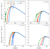 |
Fig. 1. Power-law spectrum Fν ∝ ν−2 absorbed by a distribution of column densities. The distribution Θ is drawn from a lognormal with avgΘ = 21.0 (upper left panel), 22.0 (upper right), 23.0 (lower left), and 24.0 (lower right) dex [cm−2]. Distributions for different stdΘ are also shown in each panel: stdΘ = 0.5 (dot-dashed green line), 0.3 (solid red), 0.2 (dotted yellow), 0.01 (solid cyan). The dashed blue line shows an absorbed flat spectrum |

The discrepancy between the exact and average column density (dashed blue line in Fig. 1) solutions can be computed in terms of the ratio  . In the example shown in the upper left panel,
  is in excess of 1% at E ≤ 1 keV, amounting to 10% at 0.3 keV. The discrepancy increases exponentially at lower energies, so that it is already a few orders of magnitudes at 0.1 keV. This situation worsens for all values of avgΘ > 21.0 and stdΘ ≫ 0.01 dex.
We computed and tabulated the correct absorption AΘ for all values of avgΘ ∈ [19.5, 25.5] and stdΘ ∈ [0, 1]. The table is multiplicative so that its entries, as a function of energy, are to be multiplied by any unabsorbed spectrum. The XSPEC table provides instead the quantity −lnAΘ so that, for instance, for AΘ = e−2 the XSPEC entry provides the value 2. The XSPEC class of this table is an etable, and it can also be used as a multiplicative model when loaded through the command etable{ < TABLE_NAME >}.
3. Discussion
We demonstrate the efficacy of the disnht model in retrieving the correct values by simulating a set of 100 lines of sight encompassing a distribution of column densities NH. The NH distribution Θ is drawn from a lognormal with mean value avgΘ = 23.30 and standard deviation stdΘ = 0.35. The avgΘ and stdΘ recomputed after the extraction are 23.25 and 0.34 dex, respectively. For each NH, we generated a mock spectrum using the fakeit tool of XSPEC. We built the spectrum from a collisionally ionized plasma model (APEC hereafter; Smith et al. 2001) at a temperature TAPEC = 1 keV and ISM metal abundances (taken from Lodders 2003), absorbed by neutral material, aiming to emulate the observation of a large region of diffuse emission from the hot phase of the ISM in the midplane of the Milky Way. We set the exposure time of each observation to 1 ks. The instrumental response matrix and ancillary files were taken from XMM-Newton observations of the Galactic center region with the EPIC-PN camera (Ponti et al. 2015). After simulating each spectrum individually, we summed the spectra. The resulting spectrum is shown in Fig. 2. The best-fit values of the disnht × APEC model are reported in Table 1. Both the simulated distribution of column densities and the emission model are reproduced by the disnht model best-fit parameters within the statistical uncertainties, holding a C statistics of ∼964 over 975 degrees of freedom. The tbabs × APEC best-fit model instead provides a column density of the absorbing material (Wilms et al. 2000) of 3.29 × 1022 cm−2, about an order of magnitude lower than the mean of the simulated (log-)distribution. Furthermore, when the disnht model is used, the retrieved temperature and metallicity of the emission component are consistent with a kT = 1 keV collisionally ionized plasma with solar abundances, whereas by using the tbabs model, the plasma characterization (kT = 1.56 ± 0.03 keV, Z = 1.7 ± 0.2 Z⊙) significantly differs from the originally set characterization. The C statistics held by the best-fit tbabs*APEC model is 1594.4 over 976 degrees of freedom. There is thus an overall improvement of the disnht model with respect to tbabs in terms of describing the absorption and (consequently) the emission properties of the spectrum and of the statistical goodness of the fit, at the expense of an additional degree of freedom.
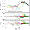 |
Fig. 2. Simulated spectrum absorbed by a lognormal distribution of column densities. The emission model is an APEC at T = 1 keV and solar abundances (Lodders 2003). The mock data are the sum of 100 simulated APEC absorbed by different column density values of the neutral material extracted from a lognormal distribution. The solid lines show disnht models with avgΘ values: 23.25 (best fit) and different stdΘ 0.50 (green), 0.33 (red, best fit), 0.20 (yellow), and 0.01 (cyan). The dashed blue line show the same emission model absorbed by a single column density equal to avgΘ = 23.25 (with best-fit kT = 1.5 keV). Residuals χ ≡ (data − model)/error and ratios data/model are shown in the central and lower panel, respectively. |
Best-fit parameters from the spectral fit of the mock data.
3.1. Lognormal distribution approximation
The disnht model is also already provided and precomputed as an interpolation between the discrete entries of a two-dimensional table. Each dimension of this table corresponds to one degree of freedom of the model. The physical distribution of column density in space or time can be arbitrarily complex to model in terms of number of parameters required to describe it analytically. The (log-)normal distribution, if applicable, offers the advantage of providing physical insight rather than just a mathematical description and also of requiring a minimal amount of free parameters: a mean and a dispersion value. Is a (log-)normal distribution a sufficiently good representation of the column density distribution? We considered the assumption as sufficiently good by testing different observed column density distributions against a lognormal with the same mean, standard deviation, and number of elements as the real distribution, through a Kolmogorov-Smirnov test. The approximation is valid for rejection probabilities of the null hypothesis (of the two distributions to have been drawn by the same one) higher than 0.05. We drew real distributions from the all sky NH maps of HI4PI Collaboration (2016). We considered this map representative of the physical column density at high Galactic latitudes b > 10deg. We built column density sets extracted over circular regions of different dimension to test our assumption over different angular scales. For each extraction radius, we drew 1000 sets centered at random positions in the sky at b > 10deg. From every set, we obtained a probability of the set to be described by a lognormal distribution. We rejected the hypothesis for p-values lower than 0.05. The distributions of p-values obtained over sets at different angular scales are shown in Fig. 3 for all p-values higher than 10−5. The original NH map has a resolution of ≃3.4′. Larger angular scales then encompass a larger number of set elements. For instance, the ∼0.1 (1.0) πdeg2 extraction region encompass 30 (300) pixels. As shown in Fig. 3, the column density distributions are generally consistent with a lognormal one up to ∼1deg radius, with the corresponding distribution of p-values peaking at p > 0.05. For larger regions, the real distribution starts to significantly deviate from lognormal. From a deeper inspection, this is due in most cases to an NH distribution resembling a sum of a few lognormal distributions corresponding to portions at small scales encompassed within a single region. The non-negligible width of these distributions makes a solution for the absorption computed from a single lognormal distribution still preferable to a correction by a single (average) value of column density. Similarly, the same test performed over the Galactic center column density map shows consistency of the lognormal assumption up to a 6′ radius angular scale, with larger regions deviating from a single lognormal. The scale that limits the validity of the lognormal approximation has to depend in general on the angular power spectrum of the column density fluctuations (and thus on the medium properties) and on the highest angular resolution used to sample the column density across the sky.
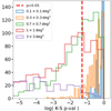 |
Fig. 3. Goodness of the approximation with a lognormal distribution in terms of Kolmogorov-Smirnov p-value distributions (log10 scale). The vertical red line shows pKS = 0.05. The Kolmogorov-Smirnov test is run over column density sets extracted from a circular region of different areas in the NH all sky maps of HI4PI Collaboration (2016). |
3.2. Deviations from single column density absorption models
So far, we have demonstrated that (i) there are several cases of significantly broad column density distributions, produced by averaging over a large enough sky area; (ii) in many of these cases, the distribution of column densities can be approximated with a lognormal distribution; and (iii) this approximation leads to a more precise characterization of the absorption spectrum in terms of statistical power and accuracy of the best-fit values. To further demonstrate the importance of adopting a more complex model than only a single exponential function of the column density and also to assess when the latter is still a good enough approximation to the spectrum, we computed the discrepancy between the two methods in terms of the quantities AΘ and  that we introduced in Sect. 2. Provided that the limit for small stdΘ of the disnht model gives the tbabs solution, the fractional (percent) deviation of
  with respect to AΘ is
 (3)
(3)
and provides a means to distinguish when the two models describe a significantly different absorption spectrum and to what extent. We quantified the fractional deviation at energy 0.3 keV. At lower (higher) energies, the models will deviate more (less). We studied the deviation for a grid of parameters in the ranges avgΘ ∈ [19.5; 23.0] using a 0.25 dex step and stdΘ ∈ [0.02; 0.22] using a 0.02 dex step. The results are shown in Fig. 4. Because of the exponential form, the difference between a negligible correction and an important correction is very large, even in log scale. We thus compressed the color scale to highlight corrections between 1 and 30% (+100% corresponding to a factor 2). A ∼1% correction may be statistically significant in a spectrum with a high signal-to-noise ratio. White regions of the parameter space indicate a negligible difference between the disnht and tbabs models. For these parameters, the latter model is statistically favorable in the absence on priors on the distribution because it requires only one (less) free parameter. We then plot in Fig. 4 the points describing the column density distributions in the random regions extracted from the maps already considered in this work for the upper bound angular scales where the lognormal approximation is verified, namely 1deg × 1deg for the HI4PI Collaboration (2016) map (red dots) and 6′×6′ for the Molinari et al. (2011) Galactic center map (blue dots). Figure 4 shows that for the majority of the high Galactic latitude regions, the tbabs model provides a good solution to the absorption because the column densities of the absorbing material are lower on average than for lines of sight passing through the disk. Furthermore, the smoother absorbing medium at high Galactic latitudes is distributed close around the mean value. The importance of the correction provided by the disnht model clearly increases toward the upper right corner of the plot (i.e., for increasing average column density, but also for increasing scatter around the mean). However, even at high latitude, there are regions that require the non-negligible correction provided by the disnht model. The situation is drastically different for Galactic center observations and in general throughout the Galactic disk. In these regions, both the average column density and the scatter around the mean increase by orders of magnitude. In this context, the high average value causes the absorption to be different than the tbabs model even for narrower distributions, and the correction factor is very large (i.e.,  ) already at 0.3 keV.
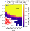 |
Fig. 4. Percent deviation |
4. Conclusions
We have presented a model for the absorption of soft X-ray spectra in the case that photons are collected from different lines of sight holding a broad distribution of column density values. After showing the efficacy of the model in retrieving the absorption properties of the spectrum, we proved that several cases exist for which it is relevant to consider it. In these cases, the assumption of an absorption spectrum described by a single column density value breaks. We have proven that in these cases, the lognormal distribution is a fair approximation to the physical distribution. The absorption model we proposed is computed by assuming that a constant layer of emission is absorbed by a distribution of column densities. This is a rather simple assumption compared to the general case, in which emission from a plasma is expected to deviate from homogeneity regardless of absorption. However, our goal is to focus on the modeling of the absorption of the spectrum, rather than on its emission. In general, whenever the source emission can be considered smooth with respect the angular scale of the absorption medium fluctuations, the disnht model is valid and provides a better description of the absorbing medium with respect to a single-value column density model. However, in case of a nonsmooth underlying emission, a correction for the column density distribution is still to be preferred to a simple average-value analysis of the absorption in terms of result accuracy for large enough column density distributions. We expect the proposed model to be relevant for current and future generation of X-ray imaging telescopes furnished with survey capabilities and large fields of view, such as eROSITA Merloni et al. (2012), Predehl et al. (2021) and Athena (Nandra et al. 2013).
The model is made available either through a python code to compute the absorption spectrum given an arbitrary column density distribution, or precomputed under the assumption of a lognormal distribution both in ascii and .fits tables (etable, XSPEC readable) formats2.
Acknowledgments
We thank our anonymous reviewer for the helpful comments on the manuscript. N.L. and G.P. acknowledge financial support from the European Research Council (ERC) under the European Union’s Horizon 2020 research and innovation program HotMilk (grant agreement No. [865637]). S.B. acknowledges financial support from the Italian Space Agency (grant 2017-12-H.0).
References
- Anders, E., & Grevesse, N. 1989, Geochim. Cosmochim. Acta, 53, 197 [Google Scholar]
- Asplund, M., Grevesse, N., Sauval, A. J., & Scott, P. 2009, ARA&A, 47, 481 [NASA ADS] [CrossRef] [Google Scholar]
- Balucinska-Church, M., & McCammon, D. 1992, ApJ, 400, 699 [Google Scholar]
- Bianchi, S., Piconcelli, E., Chiaberge, M., et al. 2009, ApJ, 695, 781 [Google Scholar]
- Bianchi, S., Ponti, G., Muñoz-Darias, T., & Petrucci, P.-O. 2017, MNRAS, 472, 2454 [Google Scholar]
- Cheng, Y., Wang, Q. D., & Lim, S. 2021, MNRAS, 504, 1627 [NASA ADS] [CrossRef] [Google Scholar]
- Díaz Trigo, M., Parmar, A. N., Boirin, L., Méndez, M., & Kaastra, J. S. 2006, A&A, 445, 179 [NASA ADS] [CrossRef] [EDP Sciences] [Google Scholar]
- Done, C., & Magdziarz, P. 1998, MNRAS, 298, 737 [NASA ADS] [CrossRef] [Google Scholar]
- Ferrière, K. M. 2001, Rev. Mod. Phys., 73, 1031 [NASA ADS] [CrossRef] [Google Scholar]
- Gupta, A., Mathur, S., Krongold, Y., Nicastro, F., & Galeazzi, M. 2012, ApJ, 756, L8 [CrossRef] [Google Scholar]
- HI4PI Collaboration (Ben Bekhti, N., et al.) 2016, A&A, 594, A116 [NASA ADS] [CrossRef] [EDP Sciences] [Google Scholar]
- LaMassa, S. M., Cales, S., Moran, E. C., et al. 2015, ApJ, 800, 144 [NASA ADS] [CrossRef] [Google Scholar]
- Lodders, K. 2003, ApJ, 591, 1220 [Google Scholar]
- Marchese, E., Braito, V., Della Ceca, R., Caccianiga, A., & Severgnini, P. 2012, MNRAS, 421, 1803 [NASA ADS] [CrossRef] [Google Scholar]
- Masui, K., Mitsuda, K., Yamasaki, N. Y., et al. 2009, PASJ, 61, S115 [NASA ADS] [CrossRef] [Google Scholar]
- Matt, G., Guainazzi, M., & Maiolino, R. 2003, MNRAS, 342, 422 [NASA ADS] [CrossRef] [Google Scholar]
- Merloni, A., Predehl, P., Becker, W., et al. 2012, ArXiv e-prints [arXiv:1209.3114] [Google Scholar]
- Molinari, S., Bally, J., Noriega-Crespo, A., et al. 2011, ApJ, 735, L33 [Google Scholar]
- Muno, M. P., Bauer, F. E., Baganoff, F. K., et al. 2009, ApJS, 181, 110 [CrossRef] [Google Scholar]
- Nandra, K., Barret, D., Barcons, X., et al. 2013, ArXiv e-prints [arXiv:1306.2307] [Google Scholar]
- Ponti, G., Morris, M. R., Terrier, R., et al. 2015, MNRAS, 453, 172 [Google Scholar]
- Ponti, G., Bianchi, S., Muñoz-Darias, T., et al. 2016, Astron. Nachr., 337, 512 [Google Scholar]
- Predehl, P., Andritschke, R., Arefiev, V., et al. 2021, A&A, 647, A1 [EDP Sciences] [Google Scholar]
- Puccetti, S., Fiore, F., Risaliti, G., et al. 2007, MNRAS, 377, 607 [Google Scholar]
- Risaliti, G., Miniutti, G., Elvis, M., et al. 2009, ApJ, 696, 160 [NASA ADS] [CrossRef] [Google Scholar]
- Rybicky, G., Lightman, A. P., & Domke, H. 1982, Astron. Nachr., 303, 142 [NASA ADS] [CrossRef] [Google Scholar]
- Smith, R. K., Brickhouse, N. S., Liedahl, D. A., & Raymond, J. C. 2001, ApJ, 556, L91 [Google Scholar]
- Wang, Q. D., Zeng, Y., Bogda, A., & Ji, L. 2021, MNRAS, 508, 6155 [NASA ADS] [CrossRef] [Google Scholar]
- Wilms, J., Allen, A., & McCray, R. 2000, ApJ, 542, 914 [Google Scholar]
- Wolfire, M. G., McKee, C. F., Hollenbach, D., & Tielens, A. G. G. M. 2003, ApJ, 587, 278 [Google Scholar]
- Yoshino, T., Mitsuda, K., Yamasaki, N. Y., et al. 2009, PASJ, 61, 805 [NASA ADS] [Google Scholar]
All Tables
All Figures
|
Fig. 1. Power-law spectrum Fν ∝ ν−2 absorbed by a distribution of column densities. The distribution Θ is drawn from a lognormal with avgΘ = 21.0 (upper left panel), 22.0 (upper right), 23.0 (lower left), and 24.0 (lower right) dex [cm−2]. Distributions for different stdΘ are also shown in each panel: stdΘ = 0.5 (dot-dashed green line), 0.3 (solid red), 0.2 (dotted yellow), 0.01 (solid cyan). The dashed blue line shows an absorbed flat spectrum |
| In the text | |
|
Fig. 2. Simulated spectrum absorbed by a lognormal distribution of column densities. The emission model is an APEC at T = 1 keV and solar abundances (Lodders 2003). The mock data are the sum of 100 simulated APEC absorbed by different column density values of the neutral material extracted from a lognormal distribution. The solid lines show disnht models with avgΘ values: 23.25 (best fit) and different stdΘ 0.50 (green), 0.33 (red, best fit), 0.20 (yellow), and 0.01 (cyan). The dashed blue line show the same emission model absorbed by a single column density equal to avgΘ = 23.25 (with best-fit kT = 1.5 keV). Residuals χ ≡ (data − model)/error and ratios data/model are shown in the central and lower panel, respectively. |
| In the text | |
|
Fig. 3. Goodness of the approximation with a lognormal distribution in terms of Kolmogorov-Smirnov p-value distributions (log10 scale). The vertical red line shows pKS = 0.05. The Kolmogorov-Smirnov test is run over column density sets extracted from a circular region of different areas in the NH all sky maps of HI4PI Collaboration (2016). |
| In the text | |
|
Fig. 4. Percent deviation |
| In the text | |
Current usage metrics show cumulative count of Article Views (full-text article views including HTML views, PDF and ePub downloads, according to the available data) and Abstracts Views on Vision4Press platform.
Data correspond to usage on the plateform after 2015. The current usage metrics is available 48-96 hours after online publication and is updated daily on week days.
Initial download of the metrics may take a while.