| Issue |
A&A
Volume 659, March 2022
|
|
|---|---|---|
| Article Number | A164 | |
| Number of page(s) | 7 | |
| Section | The Sun and the Heliosphere | |
| DOI | https://doi.org/10.1051/0004-6361/202142536 | |
| Published online | 22 March 2022 | |
Total reflection of a flare-driven quasi-periodic extreme ultraviolet wave train at a coronal hole boundary⋆
1
Yunnan Observatories, Chinese Academy of Sciences, Kunming 650216, PR China
e-mail: This email address is being protected from spambots. You need JavaScript enabled to view it.
2
State Key Laboratory of Space Weather, Chinese Academy of Sciences, Beijing 100190, PR China
3
University of Chinese Academy of Sciences, Beijing, PR China
Received:
27
October
2021
Accepted:
29
December
2021
Abstract
Context. A flare-driven quasi-periodic extreme ultraviolet wave train totally reflected at a coronal hole boundary was well imaged on both temporal and spatial scales by AIA/SDO.
Aims. We aim to investigate the driving mechanisms of the quasi-periodic wave train and demonstrate the total reflection effect at the coronal hole boundary.
Methods. The speeds of the incident and reflected wave trains are studied. The periodic correlation of the wave trains with the related flare is probed. We compare the measured incidence angle and the estimated critical angle.
Results. We find that the periods of the incident and reflected wave trains are both about 100 s. The excitation of the quasi-periodic wave train was possibly due to the intermittent energy release in the associated flare since its period is similar to that of the quasi-periodic pulsations in the associated flare. Our observational results show that the reflection of the wave train at the boundary of the coronal hole was a total reflection because the measured incidence and critical angles satisfy the theory of total reflection: the incidence angle is smaller than the critical angle.
Key words: shock waves / Sun: activity / Sun: corona / Sun: coronal mass ejections (CMEs) / Sun: flares
Movie is available at https://www.aanda.org
© ESO 2022
1. Introduction
As a fundamental physical phenomenon, waves of any kind can infer the physical parameters of the medium supporting them and hence provide a condition for diagnosing coronal physical parameters, such as the magnetic field strength, through seismology diagnostics techniques. The coronal seismology proposed by Uchida (1970) and Roberts et al. (1984) is one of the most critical techniques for estimating the magnetic–field strength of the solar corona, especially in the absence of direct approaches. This technique, based on the magnetohydrodynamic (MHD) waves and oscillations in the corona, has been widely used in many articles (e.g., Liu et al. 2011, 2012a; Shen et al. 2019; Zhou et al. 2021).
Coronal waves, a ubiquitous phenomenon in the solar atmosphere, were first discovered by the Extreme ultraviolet Imaging Telescope (EIT; Delaboudinière et al. 1995) on board the Solar and Heliospheric Observatory (SOHO; Delaboudinière et al. 1995) and are always accompanied with energetic eruptions such as flares and coronal mass ejections (CMEs; e.g., Vršnak & Lulić 2000a,b). In on-disk observations, these disturbances always appear as a circular or semicircular wavefront globally propagating through the solar corona (Moses et al. 1997; Thompson et al. 1998). They often have a lifetime ranging from 2 to 70 min and are characterized by radial propagating motion with speeds of 200−1500 km s−1 (Nitta et al. 2013). These extreme ultraviolet (EUV) waves are strongly considered to be driven by the CME. Nonetheless, without a related CME, some observations have indicated that there are some EUV waves closely associated with flares (Kumar et al. 2016; Kumar & Innes 2015). Early observations indicated that most of the EUV waves are single-pulse, diffuse wavefronts extending across a significant fraction of the solar corona. However, more detailed information on these waves has been gathered by the high spatio-temporal resolution Atmospheric Imaging Assembly (AIA; Lemen et al. 2012) telescope on board the Solar Dynamics Observatory (SDO; Pesnell et al. 2012). These new features, such as the bimodal composition with both wave and non-wave components (Zhukov & Auchère 2004; Patsourakos & Vourlidas 2012; Zong & Dai 2017), allow their physical interpretations to be made from a converged view (i.e., a fast-mode magnetosonic wave component travels ahead of a non-wave component). These bimodal compositions have been predicted in the two-dimensional MHD model (e.g., Chen et al. 2002). Three-dimensional global MHD simulations further confirm a bimodal composition of an outer, faster-mode magnetosonic wave component and an inner, CME compression front (e.g., Cohen et al. 2009; Downs et al. 2012). More convincing evidence comes from the off-limb events, which indicate that a faster EUV wavefront separates from a CME flank and propagates freely on the solar surface once the CME has propagated away sufficiently far from the Sun (Ma et al. 2011; Chen & Wu 2011; Shen & Liu 2012a; Shen et al. 2013, 2014; Zhou et al. 2021), resulting in a bifurcation structure in time-distance stack plots.
Recently, a new type of EUV wave train with multiple wavefronts propagating across the solar surface has been reported, albeit only in sporadic cases (Liu et al. 2012b; Kumar et al. 2017; Shen et al. 2019; Zhou et al. 2021). According to the statistic from Shen et al. (2022), these EUV wave trains travel away from the flare kernel with speeds ranging from 370−1100 km s−1 and with a period in the range of 36−240 s. Considering that the amplitude and velocity of these waves are not within the range of quasi-periodic fast propagating (QFP) wave trains channeled in open or closed loops but are similar to the classical EUV wave, Shen et al. (2022) classify these wave trains as broad wave trains and QFP wave trains as narrow wave trains. Furthermore, they can excite the oscillation of the cavity and filament, which are also widely observed in the classical EUV waves. Regarding the driving mechanism of the quasi-periodic EUV wave train, there are several possible interpretations: for example, they could be driven by downward and lateral CME compression (Liu et al. 2012b) or by the unwinding motion of the helical filament structures (Shen et al. 2019). This divergence may be caused by the limitation of the observational case, and as such it is hard to study the driving mechanisms in a detailed and comprehensive way. For detailed discussions about these two types of wave trains, we refer readers to the recent review by Shen et al. (2022).
True wave characteristics, such as refractions, reflections, and transmissions, have manifested in observations and simulations when a wave interacts with a region that exhibits a sudden density drop, such as coronal holes (CHs; Veronig et al. 2006; Schmidt & Ofman 2010; Shen & Liu 2012b; Olmedo et al. 2012; Kumar et al. 2016, 2017; Liu et al. 2018) and active regions (ARs; Ofman & Thompson 2002; Shen et al. 2013; Miao et al. 2019). Reflection evidence of an EUV wave at the boundary has even been observed in radio dynamic spectra (Mancuso et al. 2021). However, total reflection, a basic phenomenon in wave theory, had not yet been identified or detected in an EUV wave. Recently, Piantschitsch & Terradas (2021) used an extended theoretical approach, based on a linear theory that treats EUV waves as fast-mode MHD waves, to investigate the geometrical properties of secondary waves caused by the interaction between the oblique incoming waves and CHs. Their results show that the second waves’ geometrical properties depend on the incidence angle of the incoming waves to the CH boundaries and the plasma density contrasts, ρc, between the areas inside and outside the CH. This allows us to determine whether the secondary waves are partially or totally reflected at the CH boundaries. In this paper we report, for the first time, direct observational evidence of the total reflection that occurred on 22 December 2015, in which an EUV wave train emanated from a flare kernel and was totally reflected by a remote southern polar CH. The present study focuses on the driving mechanism of the EUV wave train, its propagation, and its interaction with the CH. The used observational data are described in Sect. 2, results are presented in Sect. 3, and discussions and conclusions are given in Sect. 4.
2. Observations and data reduction
The event was recorded by the AIA (Lemen et al. 2012) on board the SDO. During our observing time interval, AIA/SDO provided continuous full-disk observations of the solar chromosphere and corona in seven EUV channels, spanning a temperature range from approximately 2 × 10⁴ K to over 2 × 10⁷ K. We mainly used the 171 Å (Fe IX; characteristic temperature: 0.6 × 10⁶ K), 193 Å (Fe XII, XXIV; characteristic temperature: 1.6 × 10⁶, 2 × 10⁷ K), and 211 Å (Fe XIV; characteristic temperature: 2 × 10⁶ K) images, since the evolutional processes are observed in these three cooler passbands but are completely absent in the other AIA channels. The time cadence and pixel size of the AIA images are 12 s and 0.6″, respectively. All of the AIA images used here were calibrated with the standard procedure available in the SolarSoftWare package provided by the instrument team. The Geostationary Operational Environmental Satellite (GOES) soft X-ray 0.5−4.0 Å and 1.0−8.0 Å fluxes were used to analyze the periodicity pulsation of the flare. In addition, Large Angle and Spectrometric COronagraph (LASCO; Brueckner et al. 1995) images were used to portray the associated CME. To enhance the moving feature of the wave front, we utilized the running-difference images (i.e., each image was subtracted from the previous one) to study the wave trains’ evolution. To visualize the obtained signatures of the wave train, we used the wavelet analysis method (Torrence & Compo 1998) to investigate the periodicity of the wave train and flare. We performed differential emission measure (DEM) analysis using the inversion code developed by Hannah & Kontar (2012) to estimated the plasma density inside and outside the CH. The DEM inversion was done at 03:22 UT, ten minutes before the incident wave trains arrived at the CH boundary. Additionally, we used the Collection of Analysis Tools for Coronal Holes (CATCH) algorithm developed by Heinemann et al. (2019), which applies the intensity gradient along the CH boundary to modulate the extraction threshold, to extract the CH boundary.
3. Results
The event occurred close to the eastern solar limb of NOAA AR 12473 on 22 December 2015. It is associated with an M1.6 solar flare, whose start, peak, and end times were at about 03:15 UT, 03:34 UT, and 03:48 UT, respectively (see Fig. 1e). In addition, a jet-like CME with an average speed of 260 km s−1 was observed by the LASCO/C2 during the eruption (see Fig. 1d)1. An overview of the eruption source region dominated with some closed and open loops (see the enlarged view of Fig. 1c) is presented in Figs. 1a and b. In this region there was a large southern polar CH, whose boundaries, determined using the CATCH software, are also indicated in Figs. 2 and 5a and b1. The CH regions always manifest as dark structures in the EUV and X-ray emission in comparison to the peripheral solar corona because of the reduction in density and temperature caused by plasma depletion in these regions (e.g., Heinemann et al. 2019). During the rising phase of the flare, an EUV wave train, significantly different from the classic EIT wave that manifests as a single large-scale quasi-circular propagating front, emanated from the flare kernel and interacted with the distant CH. Further distinctions between the EUV and EIT waves are discussed in the reviews by Zhukov (2011) and Liu & Ofman (2014). Recent investigations have indicated that the temperature distribution of the CH has a dominant component centered around 0.9 MK and a secondary, smaller component at 1.5−2.0 MK (Saqri et al. 2020).
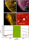 |
Fig. 1. Overview of the event. Panels a, b, and d: are AIA 171 Å, AIA 211 Å and LASCO/C2 snapshots, respectively. The field of view of panel c is marked by the white box in panel a. The incident and reflected wave trains are tracked with the two sectors indicated as S1 and S2, and the green line marks the location of the CH boundary in panel b. Panel e: solar soft X-ray recorded by the GOES in 0.5−4.0 Å (red) and 1.0−8.0 Å (blue). The green region marks the start and end time of the flare in NOAA AR 12473. |
3.1. Kinematics of the quasi-periodic EUV wave train
We mainly analyzed the time sequence of 193 Å running-difference images taken during the flare to show the overall evolutionary and interactional process, since the evolutionary processes are similar in the 171 Å and 211 Å images (see the animation available in the electronic supplementary material). The violent eruption launched multiple striking arc-shaped wavefronts running along the solar surface. Figure 2 displays the selected running-difference images in those 193 Å images, showing the multiple successive wavefronts during the impulsive phase. The first wavefront appeared at around 03:22 UT, about 7 min after the onset of the flare. Following the first wavefront, at least three successive wavefronts were detected; these wavefronts are also clearly seen in the 171 Å and 211 Å running-difference images, suggesting that the responsible plasma was in the range of these three channels’ peak response temperature of 0.6−2.0 MK. If we carefully observe the animation and Fig. 2, we can see that the intensity of the wavefronts progressively decreases as the propagation distance increases. After arriving at the CH boundary, they showed a significant reflection feature. The deflection is with respect to the initial propagation direction (and it would be around 90°; see the animation available in the electronic supplementary material and Figs. 2d–f).
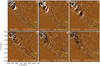 |
Fig. 2. Evolutions of the incident wave trains (top) and reflected wave trains (bottom) in 193 Å running-difference images. In each panel the red and blue lines depict the wavefronts of the incident and reflected EUV wave trains, respectively, while the green lines mark the location of the CH boundary. |
To reveal the speeds of the wave train, we selected sectors S1 and S2, as shown in Fig. 1b, in the AIA 211 Å channels. Sectors S1 (width 20°) and S2 (width 8°) were placed respectively over the incident and reflected wave train tracks, and they were selected in almost the exact directions of the corresponding wave trains. The time-distance stack plots are displayed in Fig. 3, in which one can see that the incident and reflected wave trains propagated at speeds of 730 km s−1 and 560 km s−1, respectively. Obviously, the wave train speeds are close to that of classical EUV waves but are significantly lower than that of the QFP wave train (around 2000 km s−1, as reported by Liu et al. 2011). This may reflect the difference of the fast magnetosonic speed in the quiet-Sun (as shown in the present paper) and in funnel-like magnetic structures stemming from ARs (as reported by Liu et al. 2011). Therefore, the wave train under investigation in this paper should be classified as a broad wave train, according to the classification of Shen et al. (2022). We estimated the error by making the fit ten times, placing two points along the front and deriving the average velocity (Olmedo et al. 2012). It is worth noting that only the first, strongest wavefront can be tracked from the erupting origin to the CH boundary, and there was no significant wave signal indicating that the wavefront intrudes into the CH, in contrast to what was reported by Veronig et al. (2006). The first wavefront encountered the CH boundary at about 3:32 UT (see the black arrow in Fig. 3a). Almost at the same time, the first reflected wavefront appeared (see the black arrow in Fig. 3e), followed by a series of wavefronts at the time-distance stack plot. The trailing wavefronts are so weak that they are not discernable from the time-distance stack plots in Fig. 3 after a propagation of about 200 Mm, but they can be discerned in the animation. From the time-distance stack plots, there is no significant signal of a reflected wave train in the AIA 211 Å channel, indicating that the energy of the wave train dissipates during its impingement and long-distance propagation.
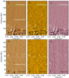 |
Fig. 3. Time-distance stack plots obtained from AIA 193 Å, 171 Å, and 211 Å running-difference images along sectors S1 (top) and S2 (bottom), as shown in Fig. 1b. The horizontal dashed lines indicate the positions for extracting signals for wavelet analysis, whereas the oblique dotted red lines depict the linear fitting results for estimating the speeds of wavefronts. The dashed green lines in the top panels represent the boundary of the southern polar CH. |
To study the origin of the EUV wave train, we applied the Morlet wavelet analysis (Torrence & Compo 1998) to analyze the periodicities of the associated impulsive M1.6 flare and the wave train. Since the Reuven Ramaty High-Energy Solar Spectroscopic Imager (RHESSI) had a data gap during the flare, a temporal derivative of GOES soft X-ray 0.5−4.0 Å and 1.0−8.0 Å fluxes were used as a proxy of the corresponding hard X-rays to analyze the periodicity of the flare according to the Neupert effect (Neupert 1968; Veronig et al. 2005; Ning & Cao 2010). Figure 4a1 displays the GOES 0.5−4.0 Å soft X-ray flux. Its temporal-derivative curve (black) is shown in Fig. 4a2. After subtracting a smoothed 100-s curve (red) from the temporal-derivative curve, we get the detrended signal, and the result is overlaid in Fig. 4a3 (see the yellow curve). Using the same method, we obtained the detrended, temporal-derivative curve of GOES 1.0−8.0 Å, and the result is overlaid in Fig. 4a4. Using such a detrended temporal-derivative curve as input, we could see that the period of the flare is about 100 s (see Figs. 4a3 and a4).
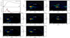 |
Fig. 4. Periodicity analysis for the wave train and the associated flare pulsation. Panels a1 and a2: GOES 0.5−4.0 Å soft X-ray flux and its temporal derivative (black curve in panel a2), respectively. The detrended intensity profile (yellow curve in panel a3) is obtained from the temporal derivative in panel a2 by subtracting its smoothed intensity profile (red curve in panel a2). The smooth and detrended derivative signal of the GOES 1.0−8.0 Å soft X-ray flux is overlaid in panel a4. The yellow curves in panels b1–c2 are smooth and detrended intensity profiles of the horizontal dashed white lines labeled “L1” and “L2” in Fig. 3, and their corresponding wave wavelet power spectra are displayed in each panel. The cross-hatched regions in panels a3–c2 indicate the cone of influence region due to the edge effect of the data, while the dotted and horizontal dashed red lines mark the 95% confidence level and the period, respectively. |
For the periodicities of the wave train, we analyzed the intensity profile extracted along the white horizontal lines marked “L1” and “L2” in Fig. 3. Using its detrended intensity profiles as input, we obtained that the average periods of the incident and reflected wave trains are 84−110 s and 88−105 s (average values are 98 s and 97 s), respectively (see Figs. 4c1 and c2). This result satisfies the characteristics of a true wave: the frequency of wave trains does not change during the propagating process or during interactions with other structures. From the wavelet analysis results, one can see that the period of the wave train is similar to that of the pulsations in the flare, suggesting that these wave trains were possibly initiated by the quasi-periodic pressure pulses launched by the intermittent energy-releasing process in the flare. Interestingly, a sub-period remains visible in Figs. 4b1–b3 and c1 for both the incident and reflected wave trains. The sub-period for the incident and reflected wave trains from Figs. 4b1–b3 and c1 are 132, 80, 103, and 180 s. In addition, a typical feature of the signature is a bifurcation and an inverse tadpole in the wavelet spectra, which is especially visible in Figs. 4b1–b3 and c2 (cf. Roberts et al. 1983, 1984; Nakariakov et al. 2004 for the tadpole in the wavelet spectrum). This specially shaped wavelet spectrum will be discussed in the next paper.
3.2. Total reflection of the quasi-periodic EUV wave train
Like any true wave, EUV waves will exhibit various behaviors when encountering a region of suddenly reduced plasma density. In addition to the total reflection, all other true wave features, such as partial reflections, refraction, and transmissions, have been observed so far. In this section we show that the wave train was totally reflected by the CH boundary.
We moved and projected S1 and S2 on the disk center, taking the projection effect on this limb event, as shown in Fig. 5a, into consideration. Considering the facts that the incidence angle equals the reflected angle (i.e., θi = θr) and the angle between the incident and reflected wave trains (two red axes of sectors S1 and S2) is about 115°, we determine that the incidence angle, θi, is about 33°, as shown in the inset in the upper-left corner of Fig. 5a. According to Piantschitsch & Terradas (2021), the critical angle, θc, depends only on the density contrast (i.e.,  ), in which ρc = ρi/ρo is the density contrast between the interior and exterior of the CH. To estimate the density contrast, we followed the method provided by Saqri et al. (2020) to perform DEM analysis for the CH; one example is shown in Fig. 5b1. All of the AIA images used for the DEM analysis were binned by 8 × 8 pixels to enhance the signal-to-noise ratio and then further deconvolved with the instrument point spread function (PSF) provided by the aia_calc_psf.pro routine to reduce the effect of instrument stray light. The plasma density can be derived from the formula
  , where EM, the emission measure, is the integration result of the DEM over the temperature range and h is the column height of the emitting plasma along the line of sight (taken here as 42 Mm and 90 Mm for the CH and the quiet-Sun region, respectively; cf. Saqri et al. 2020; Long et al. 2019). We selected ten successive segments along the CH boundary near the wave-CH interaction location and estimated the densities in the patches outside and inside the CH boundary of each individual segment. Figure 5b2 shows that the plasma densities inside and outside the CH boundary are in the range of 1.5 − 2.0 × 108 cm−3 and 2.5 − 3.0 × 108 cm−3, respectively, which are slightly lower than that reported by Saqri et al. (2020), who studied low-latitude CHs. This slight divergence is likely the result of the projection effect. The density contrast for ten segments inside and outside the CH are plotted in Fig. 5b3. From the density contrast distribution, we find that the average density contrast,
  , is about 0.62. Based on the critical angle
  (Piantschitsch & Terradas 2021), we determine the critical angle, θc, to be about 38°, which is larger than the incidence angle, θi (33°). This suggests that the incident wave train was totally reflected at the CH boundary, resulting in the secondary wave train. According to the theoretical analysis by Piantschitsch & Terradas (2021), the phase inversion angle is defined as
  . Here, we took the density contrast ρc = 0.62 and thus determined the phase inversion angle to be θp = 31°, which is in the range of 0 < θi < θp. This result further confirms that the incident wave train was totally reflected at the CH boundary.
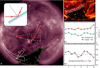 |
Fig. 5. Geometrical properties of the wave trains and the density contrast surrounding the CH boundary. a: AIA 211 Å full-disk images. The green outline represents the CH boundary extracted with the CATCH, and the sectors located on the central disk show the S1 and S2 translation and projection results. b1: plasma total emission measure in the 1.2−1.4 MK temperature range. Twenty patches were selected to estimate the density contrast surrounding the CH boundary, of which ten are inside the CH and ten are outside. b2: density inside and outside the CH shown by, respectively, the green and red lines. b3: plasma density contrast between the inside and outside CH regions. |
4. Discussion and conclusions
Using high spatio-temporal resolution imaging observations from AIA/SDO, we have presented a rare observation of a series of wavefront interactions with the southern polar CH that occurred on 22 December 2015 in NOAA AR 12473. This event is associated with an M1.6 flare and a jet-like CME. The wave train launched from the flare kernel, propagated along the solar surface, eventually reflected at the CH boundary. The speeds of the incident and reflected wave trains are 730 km s−1 and 560 km s−1, respectively. Their period is about 100 s, which is similar to that of the pulsation flare. Thus, we propose that the wave train was initiated by the intermittent energy-release process in the flare, at least in this event. The observed evolutionary process together with the fact that the incidence angle is less than the critical angle (i.e., θi < θc) suggests that the flare-initiated, quasi-periodic wave train was totally reflected at the CH boundary.
It is worth noting that most related studies have revealed that EUV waves are tightly associated with CMEs and that their relationship with flares is very weak (e.g., Veronig et al. 2008, 2010; Liu et al. 2014, 2018; Downs et al. 2021). At the same time, a considerable amount of observational evidence shows that these waves always exhibit a single diffuse wavefront. Another feature is the appearance of multiple wavefronts in a single eruption; however, such a phenomenon has only rarely been observed. According to the statistics in Shen et al. (2022), only three EUV wave trains have been reported. These wave trains have multiple wavefronts, such as the one propagating along the solar surface in the current event, and are significantly different from the narrow QFP magnetosonic wave trains (Liu et al. 2011). The main dominant difference between the broad and narrow trains is their propagating medium: the former runs along the solar surface, whereas the latter is constrained in closed or open loops. The narrow QFP wave trains are mainly detected in the AIA 171 Å wavelengths, and sometimes in the 193 Å wavelengths. In contrast, the quasi-periodic EUV wave trains, such as classical EUV waves, are visible in AIA 171 Å, 193 Å, and 211 Å wavelengths, suggesting different temperature ranges. More detailed information about these two types of wave trains can be found in a recent review (Shen et al. 2022, and references therein). These differences indicate that the observed wave train in the current event is a rare quasi-periodic wave train. In the scenario of a piston-driven shock, the wavefront should decouple from the driver, resulting in a single wavefront propagating freely on the solar surface. A single erupting jet-like CME as a driver cannot excite multiple successive wavefronts, meaning it is unlikely that the observed EUV wave train was launched by a jet-like CME. Due to the similar period of the flare pulsations and the wave train, we are inclined to believe that it was initiated by the quasi-periodic pressure pulses launched by the intermittent energy-releasing process in the flare. As we have already mentioned, EUV waves, characterized by a single wavefront, are usually initiated by a CME and generally have a weak connection with flares. The present study has shown strong evidence that EUV waves can also be excited impulsively by the quasi-periodicity of a flare. Recently, Zhou et al. (2021) reported a similar example: multiple consecutive wavefronts propagating continuously inside a CME bubble that had already attained developmental completion. This event is also hard to explain using CME expansion. The appearance of the first wavefront in the event analyzed here has a delay of several minutes relative to the onset time of the flare. A possible explanation is that the wave needs time to build up a large amplitude or shock to be observed.
Observational studies of the interaction of EUV waves with CHs are scarce, but the appearance of the secondary waves is found to be a pretty frequent phenomenon when the waves interact with CHs or ARs (Wang 2000; Gopalswamy et al. 2009; Liu et al. 2019). These observational findings were verified via numerical simulation (Piantschitsch et al. 2017, 2018a,b; Afanasyev & Zhukov 2018). In accordance with these observational and simulation-wave-like features, we can confidently confirm the interpretation that it is a fast-mode MHD wave. However, as we have already mentioned, a totally reflected wave train is a basic behavior of waves and has hardly ever been observed in the solar corona. Studying the wave-CH interaction and its secondary waves can provide a great deal of information about the CHs themselves, particularly their boundaries. Because of that, (i) the observed CH areas are well correlated with the solar wind speed measured in situ at 1 AU, which is of crucial importance for space weather forecasting models, and (ii) accurate extraction of the boundaries of the CHs is the premise of investigating the photospheric magnetic field encompassed by the CH region, which is strongly correlated with the CH area (Heinemann et al. 2018a,b). As depicted in the inset of Fig. 5, the incidence angle is about 33°. Using the method provided by Piantschitsch & Terradas (2021), we determine the critical angle of the wave train to be about 38°, which is significantly larger than the incidence angle, providing strong evidence that the incident wave train was indeed totally reflected by the southern polar CH. Recently, based on a few statistical studies, it has been shown that the density contrast at the CH boundary is in the range 0.1−0.6 (Saqri et al. 2020; Heinemann et al. 2019) and the corresponding critical angle, θc, is in the range 39° −72° (Piantschitsch & Terradas 2021). This more representative statistical result further proves that the wave train was totally reflected at the CH boundary since it is larger than the incidence angle, θi, in the current event.
The wave-CH interactions allow us to study the influence of the CH on wave parameters, such as the velocity and the amplitude (Muhr et al. 2010; Olmedo et al. 2012; Liu et al. 2018; Hu et al. 2019). The observed secondary wave signals are usually weak, resulting in the parameters of the measured secondary waves being relatively rough and of low quality. Therefore, studying more clearly captured examples of wave-CH interactions can help us deepen our understanding of the influence of CHs on coronal waves and gather more information about CHs.
Movie
Animation Access Supplementary Material
Acknowledgments
We want to thank the anonymous referee for his/her many valuable suggestions and comments for improving the quality of this article. We also thank Prof. Dr. Astrid M. Veronig and Dr. Stephan G. Heinemann for data processing and useful suggestions. Moreover, the authors want to acknowledge SDO/AIA, GOES, and SOHO/LASCO science teams for providing the data. This work is supported by the Natural Science Foundation of China (12173083, 11922307, 11773068, 11633008), the Yunnan Science Foundation for Distinguished Young Scholars (202101AV070004), the National Key R&D Program of China (2019YFA0405000), the Specialized Research Fund for State Key Laboratories and the West Light Foundation of Chinese Academy of Sciences.
References
- Afanasyev, A. N., & Zhukov, A. N. 2018, A&A, 614, A139 [NASA ADS] [CrossRef] [EDP Sciences] [Google Scholar]
- Brueckner, G. E., Howard, R. A., Koomen, M. J., et al. 1995, Sol. Phys., 162, 357 [NASA ADS] [CrossRef] [Google Scholar]
- Chen, P. F., & Wu, Y. 2011, ApJ, 732, L20 [Google Scholar]
- Chen, P. F., Wu, S. T., Shibata, K., & Fang, C. 2002, ApJ, 572, L99 [Google Scholar]
- Cohen, O., Attrill, G. D. R., Manchester, W. B., IV, & Wills-Davey, M. J. 2009, ApJ, 705, 587 [NASA ADS] [CrossRef] [Google Scholar]
- Delaboudinière, J. P., Artzner, G. E., Brunaud, J., et al. 1995, Sol. Phys., 162, 291 [Google Scholar]
- Domingo, V., Fleck, B., & Poland, A. I. 1995, Sol. Phys., 162, 1 [Google Scholar]
- Downs, C., Roussev, I. I., van der Holst, B., Lugaz, N., & Sokolov, I. V. 2012, ApJ, 750, 134 [NASA ADS] [CrossRef] [Google Scholar]
- Downs, C., Warmuth, A., Long, D. M., et al. 2021, ApJ, 911, 118 [CrossRef] [Google Scholar]
- Gopalswamy, N., Yashiro, S., Temmer, M., et al. 2009, ApJ, 691, L123 [Google Scholar]
- Hannah, I. G., & Kontar, E. P. 2012, A&A, 539, A146 [NASA ADS] [CrossRef] [EDP Sciences] [Google Scholar]
- Heinemann, S. G., Temmer, M., Hofmeister, S. J., Veronig, A. M., & Vennerstrøm, S. 2018a, ApJ, 861, 151 [NASA ADS] [CrossRef] [Google Scholar]
- Heinemann, S. G., Hofmeister, S. J., Veronig, A. M., & Temmer, M. 2018b, ApJ, 863, 29 [NASA ADS] [CrossRef] [Google Scholar]
- Heinemann, S. G., Temmer, M., Heinemann, N., et al. 2019, Sol. Phys., 294, 144 [NASA ADS] [CrossRef] [Google Scholar]
- Hu, H., Liu, Y. D., Zhu, B., et al. 2019, ApJ, 878, 106 [CrossRef] [Google Scholar]
- Kumar, P., & Innes, D. E. 2015, ApJ, 803, L23 [NASA ADS] [CrossRef] [Google Scholar]
- Kumar, P., Innes, D. E., & Cho, K.-S. 2016, ApJ, 828, 28 [Google Scholar]
- Kumar, P., Nakariakov, V. M., & Cho, K.-S. 2017, ApJ, 844, 149 [Google Scholar]
- Lemen, J. R., Title, A. M., Akin, D. J., et al. 2012, Sol. Phys., 275, 17 [Google Scholar]
- Liu, W., & Ofman, L. 2014, Sol. Phys., 289, 3233 [Google Scholar]
- Liu, W., Title, A. M., Zhao, J., et al. 2011, ApJ, 736, L13 [NASA ADS] [CrossRef] [Google Scholar]
- Liu, W., Ofman, L., Nitta, N. V., et al. 2012a, ApJ, 753, 52 [NASA ADS] [CrossRef] [Google Scholar]
- Liu, W., Berger, T. E., & Low, B. C. 2012b, ApJ, 745, L21 [Google Scholar]
- Liu, R., Wang, Y., & Shen, C. 2014, ApJ, 797, 37 [NASA ADS] [CrossRef] [Google Scholar]
- Liu, W., Jin, M., Downs, C., et al. 2018, ApJ, 864, L24 [Google Scholar]
- Liu, R., Wang, Y., Lee, J., & Shen, C. 2019, ApJ, 870, 15 [Google Scholar]
- Long, D. M., Jenkins, J., & Valori, G. 2019, ApJ, 882, 90 [CrossRef] [Google Scholar]
- Ma, S., Raymond, J. C., Golub, L., et al. 2011, ApJ, 738, 160 [CrossRef] [Google Scholar]
- Mancuso, S., Bemporad, A., Frassati, F., et al. 2021, A&A, 651, L14 [NASA ADS] [CrossRef] [EDP Sciences] [Google Scholar]
- Miao, Y. H., Liu, Y., Shen, Y. D., et al. 2019, ApJ, 871, L2 [NASA ADS] [CrossRef] [Google Scholar]
- Moses, D., Clette, F., Delaboudinière, J. P., et al. 1997, Sol. Phys., 175, 571 [NASA ADS] [CrossRef] [Google Scholar]
- Muhr, N., Vršnak, B., Temmer, M., Veronig, A. M., & Magdalenić, J. 2010, ApJ, 708, 1639 [NASA ADS] [CrossRef] [Google Scholar]
- Nakariakov, V. M., Arber, T. D., Ault, C. E., et al. 2004, MNRAS, 349, 705 [NASA ADS] [CrossRef] [Google Scholar]
- Neupert, W. M. 1968, ApJ, 153, L59 [NASA ADS] [CrossRef] [Google Scholar]
- Ning, Z., & Cao, W. 2010, ApJ, 717, 1232 [NASA ADS] [CrossRef] [Google Scholar]
- Nitta, N. V., Schrijver, C. J., Title, A. M., & Liu, W. 2013, ApJ, 776, 58 [Google Scholar]
- Ofman, L., & Thompson, B. J. 2002, ApJ, 574, 440 [Google Scholar]
- Olmedo, O., Vourlidas, A., Zhang, J., & Cheng, X. 2012, ApJ, 756, 143 [Google Scholar]
- Patsourakos, S., & Vourlidas, A. 2012, Sol. Phys., 281, 187 [NASA ADS] [Google Scholar]
- Pesnell, W. D., Thompson, B. J., & Chamberlin, P. C. 2012, Sol. Phys., 275, 3 [Google Scholar]
- Piantschitsch, I., & Terradas, J. 2021, A&A, 651, A67 [NASA ADS] [CrossRef] [EDP Sciences] [Google Scholar]
- Piantschitsch, I., Vršnak, B., Hanslmeier, A., et al. 2017, ApJ, 850, 88 [Google Scholar]
- Piantschitsch, I., Vršnak, B., Hanslmeier, A., et al. 2018a, ApJ, 857, 130 [Google Scholar]
- Piantschitsch, I., Vršnak, B., Hanslmeier, A., et al. 2018b, ApJ, 860, 24 [Google Scholar]
- Roberts, B., Edwin, P. M., & Benz, A. O. 1983, Nature, 305, 688 [NASA ADS] [CrossRef] [Google Scholar]
- Roberts, B., Edwin, P. M., & Benz, A. O. 1984, ApJ, 279, 857 [CrossRef] [Google Scholar]
- Saqri, J., Veronig, A. M., Heinemann, S. G., et al. 2020, Sol. Phys., 295, 6 [Google Scholar]
- Schmidt, J. M., & Ofman, L. 2010, ApJ, 713, 1008 [Google Scholar]
- Shen, Y., & Liu, Y. 2012a, ApJ, 752, L23 [NASA ADS] [CrossRef] [Google Scholar]
- Shen, Y., & Liu, Y. 2012b, ApJ, 754, 7 [NASA ADS] [CrossRef] [Google Scholar]
- Shen, Y., Liu, Y., Su, J., et al. 2013, ApJ, 773, L33 [Google Scholar]
- Shen, Y., Ichimoto, K., Ishii, T. T., et al. 2014, ApJ, 786, 151 [NASA ADS] [CrossRef] [Google Scholar]
- Shen, Y., Chen, P. F., Liu, Y. D., et al. 2019, ApJ, 873, 22 [Google Scholar]
- Shen, Y., Zhou, X., Duan, Y., et al. 2022, Sol. Phys., https://doi.org/10.1007/s11207-022-01953-2 [Google Scholar]
- Thompson, B. J., Plunkett, S. P., Gurman, J. B., et al. 1998, Geophys. Res. Lett., 25, 2465 [Google Scholar]
- Torrence, C., & Compo, G. P. 1998, Bull. Am. Meteorol. Soc., 79, 61 [Google Scholar]
- Uchida, Y. 1970, PASJ, 22, 341 [NASA ADS] [Google Scholar]
- Veronig, A. M., Brown, J. C., Dennis, B. R., et al. 2005, ApJ, 621, 482 [NASA ADS] [CrossRef] [Google Scholar]
- Veronig, A. M., Temmer, M., Vršnak, B., & Thalmann, J. K. 2006, ApJ, 647, 1466 [Google Scholar]
- Veronig, A. M., Temmer, M., & Vršnak, B. 2008, ApJ, 681, L113 [NASA ADS] [CrossRef] [Google Scholar]
- Veronig, A. M., Muhr, N., Kienreich, I. W., Temmer, M., & Vršnak, B. 2010, ApJ, 716, L57 [Google Scholar]
- Vršnak, B., & Lulić, S. 2000a, Sol. Phys., 196, 157 [Google Scholar]
- Vršnak, B., & Lulić, S. 2000b, Sol. Phys., 196, 181 [Google Scholar]
- Wang, Y. M. 2000, ApJ, 543, L89 [Google Scholar]
- Zhou, X., Shen, Y., Su, J., et al. 2021, Sol. Phys., 296, 169 [CrossRef] [Google Scholar]
- Zhukov, A. N. 2011, J. Atm. Solar-Terres. Phys., 73, 1096 [NASA ADS] [CrossRef] [Google Scholar]
- Zhukov, A. N., & Auchère, F. 2004, A&A, 427, 705 [NASA ADS] [CrossRef] [EDP Sciences] [Google Scholar]
- Zong, W., & Dai, Y. 2017, ApJ, 834, L15 [NASA ADS] [CrossRef] [Google Scholar]
All Figures
|
Fig. 1. Overview of the event. Panels a, b, and d: are AIA 171 Å, AIA 211 Å and LASCO/C2 snapshots, respectively. The field of view of panel c is marked by the white box in panel a. The incident and reflected wave trains are tracked with the two sectors indicated as S1 and S2, and the green line marks the location of the CH boundary in panel b. Panel e: solar soft X-ray recorded by the GOES in 0.5−4.0 Å (red) and 1.0−8.0 Å (blue). The green region marks the start and end time of the flare in NOAA AR 12473. |
| In the text | |
|
Fig. 2. Evolutions of the incident wave trains (top) and reflected wave trains (bottom) in 193 Å running-difference images. In each panel the red and blue lines depict the wavefronts of the incident and reflected EUV wave trains, respectively, while the green lines mark the location of the CH boundary. |
| In the text | |
|
Fig. 3. Time-distance stack plots obtained from AIA 193 Å, 171 Å, and 211 Å running-difference images along sectors S1 (top) and S2 (bottom), as shown in Fig. 1b. The horizontal dashed lines indicate the positions for extracting signals for wavelet analysis, whereas the oblique dotted red lines depict the linear fitting results for estimating the speeds of wavefronts. The dashed green lines in the top panels represent the boundary of the southern polar CH. |
| In the text | |
|
Fig. 4. Periodicity analysis for the wave train and the associated flare pulsation. Panels a1 and a2: GOES 0.5−4.0 Å soft X-ray flux and its temporal derivative (black curve in panel a2), respectively. The detrended intensity profile (yellow curve in panel a3) is obtained from the temporal derivative in panel a2 by subtracting its smoothed intensity profile (red curve in panel a2). The smooth and detrended derivative signal of the GOES 1.0−8.0 Å soft X-ray flux is overlaid in panel a4. The yellow curves in panels b1–c2 are smooth and detrended intensity profiles of the horizontal dashed white lines labeled “L1” and “L2” in Fig. 3, and their corresponding wave wavelet power spectra are displayed in each panel. The cross-hatched regions in panels a3–c2 indicate the cone of influence region due to the edge effect of the data, while the dotted and horizontal dashed red lines mark the 95% confidence level and the period, respectively. |
| In the text | |
|
Fig. 5. Geometrical properties of the wave trains and the density contrast surrounding the CH boundary. a: AIA 211 Å full-disk images. The green outline represents the CH boundary extracted with the CATCH, and the sectors located on the central disk show the S1 and S2 translation and projection results. b1: plasma total emission measure in the 1.2−1.4 MK temperature range. Twenty patches were selected to estimate the density contrast surrounding the CH boundary, of which ten are inside the CH and ten are outside. b2: density inside and outside the CH shown by, respectively, the green and red lines. b3: plasma density contrast between the inside and outside CH regions. |
| In the text | |
Current usage metrics show cumulative count of Article Views (full-text article views including HTML views, PDF and ePub downloads, according to the available data) and Abstracts Views on Vision4Press platform.
Data correspond to usage on the plateform after 2015. The current usage metrics is available 48-96 hours after online publication and is updated daily on week days.
Initial download of the metrics may take a while.