| Issue |
A&A
Volume 659, March 2022
|
|
|---|---|---|
| Article Number | A83 | |
| Number of page(s) | 6 | |
| Section | Interstellar and circumstellar matter | |
| DOI | https://doi.org/10.1051/0004-6361/202142394 | |
| Published online | 09 March 2022 | |
Diffuse GeV emission in the field of HESS J1912+101 revisited
1
Guangxi Key Laboratory for Relativistic Astrophysics, School of Physics Science and Technology, Guangxi University,
Nanning
530004,
PR China
e-mail: This email address is being protected from spambots. You need JavaScript enabled to view it.
2
Department of Astronomy, School of Physical Sciences, University of Science and Technology of China,
Hefei,
Anhui
230026,
PR China
3
CAS Key Labrotory for Research in Galaxies and Cosmology, University of Science and Technology of China,
Hefei,
Anhui
230026,
PR China
4
School of Astronomy and Space Science, University of Science and Technology of China,
Hefei,
Anhui 230026,
PR China
Received:
8
October
2021
Accepted:
1
February
2022
Abstract
We have analyzed 12 years of Fermi Large Area Telescope data toward the HESS J1912+101 region. With the latest source catalog and diffuse background models, a γ-ray excess is detected with a significance of ~8σ in the energy range of above 10 GeV. It has been argued that the diffuse GeV emission in the vicinity of HESS J1912+101 are from an extended pulsar wind nebula powered by PSR J1913+1011 and also that the hard GeV emission above 10 GeV stems from the shell-type supernova remnant and is connected with the TeV emissions. Different from previous works, our analysis indicates that the H2 spatial template is preferred over the other spatial templates, suggesting that the diffuse emission component spatially correlates with the dense molecular gas. This spatial correlation favors a hadronic emission scenario, although a leptonic origin cannot be ruled out. In the hadronic scenario, the parent proton spectrum can be described by a power-law function with an index of α = 2.36 ± 0.16. Above 50 GeV, there is no emission, and the upper limits reveal a spectral cutoff or break in the parent proton spectrum that can be explained as propagation effects of cosmic rays. We argue that the parent protons may come from the candidate supernova remnant HESS J1912+101 or the young massive star cluster Mc20.
Key words: gamma rays: general / galaxies: star clusters: general / ISM: supernova remnants
© ESO 2022
1 Introduction
Supernova remnants (SNRs) are some of the most likely candidates of cosmic ray (CR) accelerators. From an observational point of view, they are also the most prominent γ-ray sources. Dozens of SNRs have been detected in both high-energy (HE) and very high energy (VHE) bands. AGILE and Fermi-LAT collaboration have detected the pion-bump feature in the medium-age SNRs (Giuliani et al. 2011; Ackermann et al. 2013), which has been regarded as a direct proof that SNRs do accelerate CR protons. On the other hand, the Air Cherenkov Telescope Arrays also detected bright TeV γ-ray emission toward the young SNRs that revealed significant shell-like structures (Aharonian et al. 2007; Albert et al. 2007). This implies that the SNRs can accelerate particles to the VHE domain. The radiation mechanism of these young SNRs is still debated. Hadronic and leptonic scenarios can both provide a reasonable fit to the observed data (see, e.g., Zirakashvili & Aharonian 2010). Yuan et al. (2012) proposed that the γ-ray emissions from SNRs can be separated into two main classes: For the young SNRs, the shocks propagate in low-density environments and the leptonic process dominates. For the old SNRs, CRs have escaped and interacted with the dense molecular clouds, and γ-rays are produced in a hadronic process in this case. However, the recent Fermi-LAT observations of HESS J1731-347 (Cui et al. 2019) found indications for an SNR-cloud interaction for the young shell-like SNRs. Thus the radiation mechanism and particle propagation process near SNRs are far from being understood, even for these extensively studied sources. In this regard, detailed multiwavelength observations toward SNRs can always deepen our understanding of these questions.
We focus on the region surrounding HESS J1912+101. HESS J1912+101 is another shell-like SNR candidate discovered by the H.E.S.S. Collaboration (H.E.S.S. Collaboration 2018). Like HESS J1731-347, it lacks a radio counterpart, but the SNR interpretation is supported by Su et al. (2017) and Reich & Sun (2019) based on the identification of associated shocked molecular gas and polarized radio emission.
The region around HESS J1912+101 is complex and hosts several potential HE γ-ray emitters in addition to the SNR candidate HESS J1912+101. The HAWC collaboration has detected 2HWC J1912+099 (Abeysekara et al. 2017), which yields a tentative indication of the extent of 0.7° and might be associated with HESS J1912+101. The medium-age radio pulsar PSR J1913+1011 at (RA, Dec) = (288.335°, 10.19°) (Morris et al. 2002) is the most plausible counterpart candidate. It is slightly offset from HESS J1912+101 at (RA, Dec) = (288.21°, 10.15°) (Aharonian et al. 2008). It is a rather energetic pulsar with a spin-down luminosity of 2.9 ×1036 erg s−1, and its distance was estimated from dispersion measurements to be 4.48 kpc (Manchester et al. 2005). This means that the pulsar is sufficiently energetic to power the HESS source (Aharonian et al. 2008). The young massive star cluster (YMC) Mc20, discovered by the GLIMPSE survey of the inner Galaxy (Mercer et al. 2005), is located within the region of the VHE γ-ray source HESS J1912+101 (Aharonian et al. 2008). It is located at (RA, Dec) = (288.10°, 9.95°) and appears as a concentration of bright stars with a radius of about 1′ at both mid-infrared and near-infrared wavelengths (Messineo et al. 2009). It contains a yellow super giant (YSG), an early WC star, and several other massive stars (Messineo et al. 2009). The mass of the star cluster is a few 103 M⊙ and the age ranges from 3 to 8 Myr (Messineo et al. 2009). The distance to the Galactic star cluster Mc20 is most likely 3.8 and 5.1 kpc (Messineo et al. 2009). The luminosity of ~4 × 1038 erg s−1 for the YSG star in the Mc20 agrees well with that of RSGC 1 (Messineo et al. 2009). The interstellar extinction and spectrophotometric distances of the YSG, the Wolf–Rayet (WR) stars, blue supergiants (BSGs), and the early-type stars are consistent, which confirms that the stellar cluster is real (Messineo et al. 2009). The mid-infrared bubble N91, which has an average radius of 5.08′ and a kinematic distance of 4.9 ± 1.1 kpc (near) or 7.3 ± 1.1 kpc (far) (Churchwell et al. 2006), is centered on the border of Mc20 in projection on the sky. Churchwell et al. (2006) suggested that dynamically formed bright bubbles N91 at mid-infrared wavelengths but not coincident with SNRs, planetary nebulae, and radio H II region probably require the massive stars to excite the polycyclic aromatic hydrocarbon (PAH) bands and a strong enough wind to evacuate a dust-free cavity.
The recent γ-ray detection of other YMCs (Ackermann et al. 2011; Yang & Aharonian 2017; Aharonian et al. 2019) makes Mc20 also a potential γ-ray source and CR accelerator. We note that Mc20 is only about 0.34° away from PSR J1913+1011. The close spatial distribution, the strong contamination from the background, and the limited resolution of γ-ray telescopes make it hard to resolve the origins of the overlapping γ-ray emissions.
In the GeV energy band, Zhang et al. (2020) argued that the diffuse GeV emission in the vicinity of the HESSJ1912+101 stems from an extended PWN powered by PSR J1913+1011. Zeng et al. (2021) reanalyzed the Fermi-LAT observations of it and found an extended source with a hard spectrum. They suggested that HESS J1912+101 may be in a peculiar stage of SNR evolution that dominates the acceleration of TeV cosmic rays.
In this work, we reanalyze this region with publicly available Fermi-LAT data. The paper is structured as follows. In Sect. 2 we present the data analysis for Fermi-LAT observations. In Sect. 3 we describe the gas distribution in the vicinity of HESS J1912+101. In Sect. 4 we discuss the possible radiation mechanisms of the γ-ray emission. Section 5 contains the discussion and conclusion.
2 Fermi-LAT data analysis
We used the Fermi-LAT Pass 8 database from August 4, 2008 (MET 239557417), to August 31, 2020 (MET 620554508), to study the GeV γ-ray emission in the region around HESS J1912+101. We considered a region of interest (ROI) with a radius of 10° centered at the position of (RA = 288.104°, Dec = 9.961°) and selected the “source” event class in an energy range from 316 MeV to 230 GeV. Both front- and back-converted photons were included. To exclude time periods in which some spacecraft event affected the data quality, we used the recommended expression (DATA_QUAL > 0)&&(LAT_CONFIG == 1). We applied a maximum zenith angle of 90° to reduce the background contamination from the Earth limb photons. We processed the data using the standard binned likelihood framework1 provided by the current Fermitools from the conda distribution2 together with the latest instrument response functions (IRFs) P8R3_SOURCE_V3.
In our background model, we include the sources in the Fermi-LAT eight-year catalog (4FGL, Abdollahi et al. 2020) within the ROI enlarged by 5°. We left the normalizations and spectral indices free for all sources within a distance of 5° from Mc20. For the diffuse background components, we used the latest Galactic diffuse model gll_iem_v07.fits and isotropic emission model iso_P8R3_SOURCE_V3_v1.txt3 and left their normalization parameters free. The complex region is located along the Galactic plane, therefore we reoptimized for the test statistic (TS) fits by setting the keyword tsmin = true.
We used the events above 10 GeV to study the spatial distribution of the γ-ray emission in the region around HESS J1912+101. All the assumed components hereafter have a power-law spectral shape. The count map in the 2.5° × 2.5° region is shown in Fig. 1, and the pixel size corresponds to 0.05° × 0.05°, smoothed with a Gaussian filter of 0.25°. Hereafter all the sky maps smoothed with this degree are only for visualization and have no effect on the analysis. The green crosses and circles show the positions of the sources from 4FGL within the region. The region around Mc20 and PSR J1913+1011, marked with black crosses, is characterized by two emission peaks in the count map. The white contours show the VHE γ-ray excess HESS J1912+101 as seen by HESS (H.E.S.S. Collaboration 2018). The tentative extension of 2HWC J1912+099 (Abeysekara et al. 2017) is marked with the yellow circle.
The distance in projection on the sky between Mc20 and PSR J1913+1011 is only 0.33°. It is rather difficult to distinguish the origin of the GeV γ-ray emission in this direction. First, we excluded the unidentified sources 4FGL J1912.7+0957, 4FGL J1913.3+1019, 4FGL J1914.7+1012, and 4FGL J1911.7+1014 from the background model and performed a background-only fitting. The corresponding background-subtracted TS image is shown in Fig. 2. Here the TS value for each pixel is defined as TS = 2(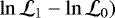 , where
  is the likelihood value of the background (null hypothesis) and
  is the likelihood value of the hypothesis for adding a source (alternative hypothesis) located in this pixel. It is obvious that both regions around Mc20 and PSR J1913+1011 have GeV γ-ray emission. We find that the most significant emission arises near PSR J1913+1011, which was studied extensively in Zhang et al. (2020). We first tested the extension of this source by replacing the point source 4FGL JJ1913.3+1019 with Gaussian disks, but found no improvement of the likelihood fitting. This is consistent with the results in Zhang et al. (2020).
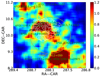 |
Fig. 1 Fermi-LAT count map above 10 GeV in the 2.5° × 2.5° region surrounding HESS J1912+101. The pixel size corresponds to 0.05° × 0.05° and is smoothed with a Gaussian filter of 0.25°. All green marks represent the 4FGL sources within the region. The VHE γ-ray excess as seen by HESS is shown as white contours, and the tentative extension of 2HWC J1912+099 is marked with the yellow circle. |
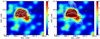 |
Fig. 2 Left: Fermi-LAT TS residual map above 10 GeV around HESS J1912+101 after subtracting the sources 4FGL J1912.7+0957, 4FGL J1913.3+1019, 4FGL J1914.7+1012, and 4FGL J1911.7+1014 from the primary model. The size is that of the 2.5° × 2.5° region smoothed with a Gaussian filter of 0.25°, and each pixel is 0.05° × 0.05°. The pluses shows the positions of PSR J1913+1011, Mc20, and N91. The crosses indicate the twobest-fit emission peaks for 4FGL J1912.7+0957 and 4FGL J1913.3+1019. The VHE γ-ray excess as seen by HESS is shown as white contours. We removed the six candidate sources labeled ps1 to ps6 from the TS map. The white contours show the TeV γ-ray emission of HESS J1912+101. Right: same TS residual map as in left panel, but the contours of the H2 column density derived in Sect. 3 are overlaid. |
2.1 Two-point source model
We note that the background point sources 4FGL J1912.7+0957 and 4FGL J1913.3+1019 are located close to HESS J1912+101 in projection on the sky. 4FGL J1913.3+1019 is reported to be associated with the PSR J1913+1011, which is only ~ 0.14° away, therefore we used the gtfindsrc tool to reoptimize the positions of the 4FGL J1912.7+0957 and 4FGL J1913.3+1019. The best-fit position is (RA = 287.98°, Dec = 9.93°) (best 1) for the first and (RA = 288.38°, Dec = 10.33°) (best 2) for the second. They are marked with crosses in Fig. 2. We hereafter relocated the two 4FGL sources in the primary background model at their best-fit positions (two-point source model). We performed a binned likelihood analysis. The derived likelihood values from the alternative hypothesis  and the Akaike information criterion (AIC, Akaike 1974) for the two-point source model are 101954 and 204068, respectively. Here the AIC is defined as AIC =
  , where k is the number of free parameters in the model, and
  is the likelihood value of the corresponding model.
2.2 Multi-point source model
We subtracted the source 4FGL J1913.3+1019 from the above two-point source model and derived the residual map shown in Fig. 3. The map revealed significant diffuse residuals in this region. We test different spatial models of these diffuse emissions in the following subsections.
As shown in Fig. 3, the white contours represent the H2 distribution derived from Sect. 3. We find another six peaks in the residual map. We therefore placed the additional six point sources, labeled ps1 to ps6 in Fig. 3, in the background model. Each component has a power-law spectral shape. We performed the binned likelihood analysis. The derived  and AIC for the multi-point source model are 101 906 and 204 008, respectively.
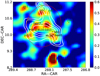 |
Fig. 3 Residual map above 10 GeV near the HESS J1912+101 region after subtracting the background sources and 4FGL J1913.3+1019. The red ellipse with a size of 0.8° × 0.6° represents the spatial model that replaces the components of 4FGL J1912.7+0957, ps2, ps5, and ps6. The white contours represent the H2 distribution. |
2.3 Spatial model for the elliptical disk
We further researched the morphology and extension of the GeV emission. We produced a series of uniform elliptical disks centered at the center of the red ellipse in Fig. 3 in the residual map with various semi-major and semi-minor axes from 0.4° to 1.0° in steps of 0.05°. We used these elliptical disks to replace the spatial components of 4FGL J1912.7+0957, ps2, ps5, and ps6 in the multi-point source model. We find that an elliptical disk with a size of 0.8° × 0.6° such as the red ellipse shown in Fig. 3 can explain the observational data best. The derived  is equal to 101 912, and the AIC is equal to 203 996.
Spatial analysis results (>10 GeV) for different templates.
2.4 HESS template
To verify whether the extended γ-ray emission is spatially correlated with the shell-like structure detected by HESS, we used the HESS significance map as the spatial model. The HESS observation template was taken from Aharonian et al. (2008), Through the binned likelihood analysis, the derived  and the AIC for the HESS spatial model are 101 920 and 204 012, respectively.
2.5 Spatial template for molecular hydrogen
To determine whether the extended GeV γ-ray emission is correlated with the gas distributions, we considered a spatial template for H2. The H2 template was produced from the carbon monoxide (CO) composite survey described in Sect. 3. After performing the binned likelihood analysis, we derived  and AIC for the spatial model of H2 of 101 909 and 203 990, respectively.
The evidence for extended emission was evaluated from the likelihood radio, , where
  is the maximum likelihood for the extended hypotheses and
  is the maximum likelihood for the referenced point-like hypotheses (Lande et al. 2012). In addition, we also compared models using the Δ AIC as the difference between the AIC of the multi-point source or the extended model and the two-point source model. The minimum Δ AIC preferres the first model. It is evident from Table 1 that the model with the H2 spatial template provides the highest TSext value and the lowest Δ AIC value. In this case, the extension component above 10 GeV has a significance of ~ 8σ. The obtained spectral parameters are a photon index of 2.27 ± 0.60 and an energy flux of (1.6 ± 0.3) × 10−10 erg cm−2 s−1.
2.6 Spectral analyses
To study the origin of the GeV emission and the underlying energy distribution of the parent particles in the region around HESS J1912+101, we derived the spectral energy distribution (SED) of the extended source 4FGL J1912.7+0957. As described in Sect. 2.5, the consistency of the γ-ray extension above 10 GeV with the derived H2 distribution shown in Fig. 3 is preferred. We therefore selected the spatial template for H2 and assumed a power-law spectral shape to extract the spectrum. As shown in Figs. 4 and 6 with red points, we derived the SED via the maximum likelihood estimation in eight logarithmically spaced bins for the γ-ray emission in the energy range of 316 MeV–230 GeV. The significance of the signal detection for each energy bin exceeds 2σ. 3σ upper limits were calculated for the energy bins with a significance lower than 2σ. The uncertainties of the diffuse emission may have some influence in the low-energy range. We tested these uncertainties by artifically varying the normalization of the Galactic diffuse emission by 6% from the best-fit value for each energy bin (Abdo et al. 2009). We estimatethe possible systematic error to be 8–18%. Statistical and systematic errors are included in the error bars shown in Figs. 4 and 6. For comparison, we also derived the SED of the point source 4FGL J1913.3+1019, shown in Fig. 4 in blue. In Fig. 4, the black data are the HESS energy flux spectra taken from HESS J1912+101 (H.E.S.S. Collaboration 2018), and the green butterfly shows the best-fit power-law model with Γ =2.64 ± 0.06 of 2HWC J1912+099 (Abeysekara et al. 2017).
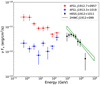 |
Fig. 4 SED of 4FGL J1912.7+0957 (red data) extracted from the H2 spatial model. Statistical and systematic errors are considered. The blue data points are derived from the 4FGL J1913.3+1019 at the best two positions, as shown in Fig. 2. The black data points represent the HESS energy flux spectra taken from HESS J1912+101, and the green butterfly shows the best-fit power-law model with Γ = 2.64 ± 0.06 of 2HWC J1912+099. |
3 Gas content around HESS J1912+101
To track the distribution of H2 surrounding the HESS J1912+101 region, we used the CO composite survey (Dame et al. 2001). We used the standard assumption of a linear relation between the velocity-integrated brightness temperature of CO 2.6 mm line, WCO, and the column density of molecular hydrogen, N(H2), meaning N(H2) = XCO × WCO (Lebrun et al. 1983). The value of the conversion factor XCO was chosen to be 2.0 × 1020 cm−2 K−1 km−1 s (Bolatto et al. 2013; Dame et al. 2001). We considered a radial velocity in the range of 50–70 km s−1 for the column density calculations of H2 (Su et al. 2017). The derived H2 column density map is shown in Fig. 5. We calculated the total mass within the cloud in each pixel according to the following expression:
 (1)
(1)
where mH is the mass of the hydrogen atom, and  is the total column density of the hydrogen atom in each pixel derived from the molecular clouds. Aangular refers to the angular area, and d is the distance of the objective region. We calculated the mass and number of the hydrogen atom in each pixel and then estimated the mass and number summations within the H2 region. Because the H2 distribution in projection on the sky is irregular, we replaced it with the elliptical disk used in Sect. 2.3 for the calculations. The total mass is estimated to be ~ 7.97 × 10⁵ M⊙. Assuming ellipsoidal geometries of the H2 spatial distribution within the GeV γ-ray emission region, we estimate the volume of the ellipsoid to be
  , with corresponding sizes of (0.8°, 0.6°) for the ellipsoidal geometries. Here r1,2 = d × θ1,2 (rad) are the semi-major and semi-minor axes of the assumed ellipse. Then the average gas number densities over the ellipsoidal volumes of the extended region were calculated to be ~79 cm−3. In addition, we calculated the H I and H II column densities using the same methods as Sun et al. (2020a,b). However, there is almost no H I and H II gas in the GeV excess region.
As shown in Fig. 3, the excess of the GeV γ-ray emission around HESS J1912+101 is spatially consistent with the high-density molecular gas distribution. This is marked with white contours. The consistency confirms the hadronic origin, that is, the emission comes from the decay of neutral pions produced by the interactions between the accelerated hadrons and the surrounding molecular gas. However, as shown in Fig. 5, the excess of the TeV γ-ray emission HESS J1912+101, marked with white contours, does not seem to be spatially consistent with the distribution of molecular gas.
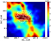 |
Fig. 5 H2 column density derived from the CO data. We integrated the gases within the velocity interval from 50–70 km s−1. The white contours are the same as in the left panel of Fig. 2. |
4 Origin of the γ-ray emission
To fit the SEDs, we used Naima4 (Zabalza 2015), which is a numerical package that allows us to implement different functions and includes tools to perform an MCMC fitting of nonthermal radiative processes to the data. Because the extended GeV emission and the molecular hydrogen gas are spatially correlated, we used a hadronic scenario in which HE γ-rays produced in the pion-decay process follow the proton-proton inelastic interactions, using the parameterization of the cross-section of Kafexhiu et al. (2014). Because the low-energy data points are poorly constrained, we used a power-law spectrum with an exponential cutoff for the parent proton distribution,
 (2)
(2)
to fit the GeV γ-ray data. This is shown by the red points in Fig. 6. We treated A, α, and Ecutoff as free parameters for the fitting. The average number density of the target protons was assumed to be 79 cm−3 as derived from the gas distributions in Sect. 3. In Fig. 6 we present the best-fit results. The derived total energy of the protons (>2 GeV) is 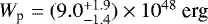 , with the index α = 2.36 ± 0.16, and Ecutoff = 1.0 ± 0.5 TeV.
As a comparison, we also predict the fluxes of γ-ray emission based on the H2 column density map, assuming the CRs have the same spectra as measured in the solar neighborhood (Aguilar et al. 2015). The fluxes are shown as the red dashed curve in Fig. 6. We found that the predicted diffuse emission in this region is significantly softer. Above 20 GeV, the emission became one order of magnitude lower than our detected emissions. We also tested the leptonic scenario in which the γ-rays are assumedto be generated via the inverse Compton (IC) scattering of relativistic electrons of the low-energy seed photons in the region around HESS J1912+101. We considered the cosmic microwave background, infrared, and optical emission calculated by Popescu et al. (2017) for the interstellar radiation field of the IC calculations. We adopted the formalism described in Khangulyan et al. (2014) to calculate the IC spectrum. We assumed a power-law distribution of the relativistic electrons with an energy above 5 GeV. In Fig. 6, the solid red curve represents the spectrum of γ-ray s from interactions of relativistic protons with the ambient gas. The solid black curve represents the total predicted γ-ray emission from the IC upscattering of the seed photons by relativistic electrons. The IC model can fit the observable data, and the corresponding maximum likelihood value is −2.8. The derived parameters for the electrons areα = 3.41 ± 0.13, and the total energy of the electrons is 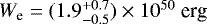 .
.
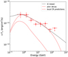 |
Fig. 6 γ-ray SED of the extended component 4FGL J1912.7+0957 is the same as in Fig. 4. The dashed red curve represents the predicted γ-ray emission assuming that the CR spectra therein are the same as those measured locally by AMS-02 (Aguilar et al. 2015). |
5 Discussion and conclusion
The region surrounding HESS J1912+101 is very complex with the bright pulsar PSR J1913+1011, the SNR candidate, and the YMC Mc20. The crowded nature and our limited understanding of the interstellar medium in this region also introduce large uncertainties in the modeling of the Galactic diffuse γ-ray background. In this case, the residuals may be due to the imperfect modeling of the diffuse background, especially considering the spatial coincidence of γ-rays and molecular gas. However, as shown in Fig. 6, the hard spectrum with an index of 2.36 is not compatible with the Galactic diffuse γ-ray background, which has an index of 2.7. The PWNe and SNRs can also be natural γ-rays emitters, and as mentioned above, hadronic and leptonic scenarios can both account for the γ-ray emissions.
The PWN scenario of the GeV emission in this region was first proposed by Zhang et al. (2020) and is discussed in detail therein. We also found that such a point source spatially coincides with the position of the pulsar. After subtracting this point source, we found a diffuse emission component. At a distance of about 4 kpc, the physical size of this source is more than 50 pc, which is quite large for typical SNRs, although we cannot entirely exclude this possibility.
Zeng et al. (2021) argued that the diffuse GeV emission stems from the shell of the SNR. The detailed spatial analysis in this work found a better spatial correlation with the gas, implying an alternative explanation, such as CR escape from the SNR that interacts with the molecular cloud. Malkov et al. (2011) argued that in a dense environment near the interacting SNR, strong ion–neutral collisions in an adjacent molecular cloud leads to Alfvén wave evanescence, which introduces fractional particle losses and results in the steepening of the energy spectrum. Su et al. (2017) also found from molecular and atomic line observations that the SNRs already interact with the molecular cloud. This shows that this effect can also address the spectral cutoff or break in the γ-ray emissions detected here. The derived total CR proton energy of about 1049 erg is also consistent with the SNR scenarios.
We also note that the YMC Mc20 is in the vicinity as well. Another explanation may therefore be the CRs that are accelerated by the interaction of the YMC with the ambient gas, as is the case in Cygnus cocoon (Ackermann et al. 2011; Aharonian et al. 2019), NGC 3603 (Yang & Aharonian 2017), W40 (Sun et al. 2020a), and RSGC 1 (Sun et al. 2020b). The significant spatial extension and hard γ-ray emission (with an index of 2.36) also show similarities with those of other YMCs. However, the spectra reveal a significant break above 50 GeV, which is significantly different from that in other YMCs. This may be due to the different acceleration ability of these systems.
In conclusion, in the vicinity of HESS J1912+101, we found a diffuse GeV emission component that is spatially correlated with the dense molecular gas. The spectra of this component can be described by a power-law function with an index of 2.36. Above 50 GeV there is no emission, and the upper limit reveals a spectral cutoff or break. The γ-ray spectrum can be described by leptonic and hadronic models alike. However, the spatial correlation with gas favors a hadronic origin. The parent protons may come both from the SNR HESS J1912+101 and the YMC Mc20. The former case is similar to other interactions in systems of SNR and molecular clouds such as W44, and the spectral break can be explained as the propagation effects of CRs. If this case is confirmed, it will add another example of YMCs as the acceleration site of CRs. The derived spectral index of 2.36 is similar to other systems like this, but the spectral break of the parent protons at about 1 TeV is significantly smaller than in other observed systems. The difference may shed light on the acceleration and propagation mechanisms of CRs near YMCs. This requires further investigations.
Acknowledgements
This work is supported by the National Natural Science Foundation of China (Grant No.12133003, 12103011, and U1731239), Guangxi Science Foundation (grant No. 2017AD22006, 2021AC19079). Rui-zhi Yang is supported by the NSFC under grants 11421303, 12041305 and the national youth thousand talents program in China.
References
- Abdo, A. A., Ackermann, M., Ajello, M., et al. 2009, ApJ, 706, L1 [NASA ADS] [CrossRef] [Google Scholar]
- Abdollahi, S., Acero, F., Ackermann, M., et al. 2020, ApJS, 247, 33 [Google Scholar]
- Abeysekara, A. U., Albert, A., Alfaro, R., et al. 2017, ApJ, 843, 40 [Google Scholar]
- Ackermann, M., Ajello, M., Allafort, A., et al. 2011, Science, 334, 1103 [NASA ADS] [CrossRef] [Google Scholar]
- Ackermann, M., Ajello, M., Allafort, A., et al. 2013, Science, 339, 807 [NASA ADS] [CrossRef] [Google Scholar]
- Aguilar, M., Aisa, D., Alpat, B., et al. 2015, Phys. Rev. Lett., 114, 171103 [CrossRef] [PubMed] [Google Scholar]
- Aharonian, F., Akhperjanian, A. G., Bazer-Bachi, A. R., et al. 2007, A&A, 464, 235 [NASA ADS] [CrossRef] [EDP Sciences] [Google Scholar]
- Aharonian, F., Akhperjanian, A. G., Barres de Almeida, U., et al. 2008, A&A, 484, 435 [NASA ADS] [CrossRef] [EDP Sciences] [Google Scholar]
- Aharonian, F., Yang, R., & de, E. 2019, Nat. Astron., 3, 561 [CrossRef] [Google Scholar]
- Akaike, H. 1974, IEEE Trans. Automat. Control, 19, 716 [Google Scholar]
- Albert, J., Aliu, E., Anderhub, H., et al. 2007, A&A, 474, 937 [NASA ADS] [CrossRef] [EDP Sciences] [Google Scholar]
- Bolatto, A. D., Wolfire, M., & Leroy, A. K. 2013, ARA&A, 51, 207 [CrossRef] [Google Scholar]
- Churchwell, E., Povich, M. S., Allen, D., et al. 2006, ApJ, 649, 759 [CrossRef] [Google Scholar]
- Cui, Y., Yang, R., He, X., Tam, P. H. T., & Pühlhofer, G. 2019, ApJ, 887, 47 [NASA ADS] [CrossRef] [Google Scholar]
- Dame, T. M., Hartmann, D., & Thaddeus, P. 2001, ApJ, 547, 792 [Google Scholar]
- Giuliani, A., Cardillo, M., Tavani, M., et al. 2011, ApJ, 742, L30 [NASA ADS] [CrossRef] [Google Scholar]
- H.E.S.S. Collaboration (Abdalla, H., et al.) 2018, A&A, 612, A8 [NASA ADS] [CrossRef] [EDP Sciences] [Google Scholar]
- Kafexhiu, E., Aharonian, F., Taylor, A. M., & Vila, G. S. 2014, Phys. Rev. D, 90, 123014 [Google Scholar]
- Khangulyan, D., Aharonian, F. A., & Kelner, S. R. 2014, ApJ, 783, 100 [Google Scholar]
- Lande, J., Ackermann, M., Allafort, A., et al. 2012, ApJ, 756, 5 [NASA ADS] [CrossRef] [Google Scholar]
- Lebrun, F., Bennett, K., Bignami, G. F., et al. 1983, ApJ, 274, 231 [NASA ADS] [CrossRef] [Google Scholar]
- Malkov, M. A., Diamond, P. H., & Sagdeev, R. Z. 2011, Nat. Commun., 2, 194 [NASA ADS] [CrossRef] [Google Scholar]
- Manchester, R. N., Hobbs, G. B., Teoh, A., & Hobbs, M. 2005, AJ, 129, 1993 [Google Scholar]
- Mercer, E. P., Clemens, D. P., Meade, M. R., et al. 2005, ApJ, 635, 560 [NASA ADS] [CrossRef] [Google Scholar]
- Messineo, M., Davies, B., Ivanov, V. D., et al. 2009, ApJ, 697, 701 [NASA ADS] [CrossRef] [Google Scholar]
- Morris, D. J., Hobbs, G., Lyne, A. G., et al. 2002, MNRAS, 335, 275 [Google Scholar]
- Popescu, C. C., Yang, R., Tuffs, R. J., et al. 2017, MNRAS, 470, 2539 [NASA ADS] [CrossRef] [Google Scholar]
- Reich, W., & Sun, X.-H. 2019, Res. Astron. Astrophys., 19, 045 [CrossRef] [Google Scholar]
- Su, Y., Zhou, X., Yang, J., et al. 2017, ApJ, 845, 48 [NASA ADS] [CrossRef] [Google Scholar]
- Sun, X.-N., Yang, R.-Z., Liang, Y.-F., et al. 2020a, A&A, 639, A80 [NASA ADS] [CrossRef] [EDP Sciences] [Google Scholar]
- Sun, X.-N., Yang, R.-Z., & Wang, X.-Y. 2020b, MNRAS, 494, 3405 [NASA ADS] [CrossRef] [Google Scholar]
- Yang, R.-z., & Aharonian, F. 2017, A&A, 600, A107 [NASA ADS] [CrossRef] [EDP Sciences] [Google Scholar]
- Yuan, Q., Liu,S., & Bi, X. 2012, ApJ, 761, 133 [NASA ADS] [CrossRef] [Google Scholar]
- Zabalza, V. 2015, Int. Cosmic Ray Conf., 34, 922 [Google Scholar]
- Zeng, H., Xin, Y., Zhang, S., & Liu, S. 2021, ApJ, 910, 78 [NASA ADS] [CrossRef] [Google Scholar]
- Zhang, H.-M., Xi, S.-Q., Liu, R.-Y., et al. 2020, ApJ, 889, 12 [NASA ADS] [CrossRef] [Google Scholar]
- Zirakashvili, V. N., & Aharonian, F. A. 2010, ApJ, 708, 965 [NASA ADS] [CrossRef] [Google Scholar]
All Tables
All Figures
|
Fig. 1 Fermi-LAT count map above 10 GeV in the 2.5° × 2.5° region surrounding HESS J1912+101. The pixel size corresponds to 0.05° × 0.05° and is smoothed with a Gaussian filter of 0.25°. All green marks represent the 4FGL sources within the region. The VHE γ-ray excess as seen by HESS is shown as white contours, and the tentative extension of 2HWC J1912+099 is marked with the yellow circle. |
| In the text | |
|
Fig. 2 Left: Fermi-LAT TS residual map above 10 GeV around HESS J1912+101 after subtracting the sources 4FGL J1912.7+0957, 4FGL J1913.3+1019, 4FGL J1914.7+1012, and 4FGL J1911.7+1014 from the primary model. The size is that of the 2.5° × 2.5° region smoothed with a Gaussian filter of 0.25°, and each pixel is 0.05° × 0.05°. The pluses shows the positions of PSR J1913+1011, Mc20, and N91. The crosses indicate the twobest-fit emission peaks for 4FGL J1912.7+0957 and 4FGL J1913.3+1019. The VHE γ-ray excess as seen by HESS is shown as white contours. We removed the six candidate sources labeled ps1 to ps6 from the TS map. The white contours show the TeV γ-ray emission of HESS J1912+101. Right: same TS residual map as in left panel, but the contours of the H2 column density derived in Sect. 3 are overlaid. |
| In the text | |
|
Fig. 3 Residual map above 10 GeV near the HESS J1912+101 region after subtracting the background sources and 4FGL J1913.3+1019. The red ellipse with a size of 0.8° × 0.6° represents the spatial model that replaces the components of 4FGL J1912.7+0957, ps2, ps5, and ps6. The white contours represent the H2 distribution. |
| In the text | |
|
Fig. 4 SED of 4FGL J1912.7+0957 (red data) extracted from the H2 spatial model. Statistical and systematic errors are considered. The blue data points are derived from the 4FGL J1913.3+1019 at the best two positions, as shown in Fig. 2. The black data points represent the HESS energy flux spectra taken from HESS J1912+101, and the green butterfly shows the best-fit power-law model with Γ = 2.64 ± 0.06 of 2HWC J1912+099. |
| In the text | |
|
Fig. 5 H2 column density derived from the CO data. We integrated the gases within the velocity interval from 50–70 km s−1. The white contours are the same as in the left panel of Fig. 2. |
| In the text | |
|
Fig. 6 γ-ray SED of the extended component 4FGL J1912.7+0957 is the same as in Fig. 4. The dashed red curve represents the predicted γ-ray emission assuming that the CR spectra therein are the same as those measured locally by AMS-02 (Aguilar et al. 2015). |
| In the text | |
Current usage metrics show cumulative count of Article Views (full-text article views including HTML views, PDF and ePub downloads, according to the available data) and Abstracts Views on Vision4Press platform.
Data correspond to usage on the plateform after 2015. The current usage metrics is available 48-96 hours after online publication and is updated daily on week days.
Initial download of the metrics may take a while.