The origin of the high metallicity of close-in giant exoplanets

S. Shibata; R. Helled; M. Ikoma

doi:10.1051/0004-6361/202142180

Home

All issues

Volume 659 (March 2022)

A&A, 659 (2022) A28

Full HTML

Free Access

Issue		A&A Volume 659, March 2022


Article Number		A28
Number of page(s)		16
Section		Planets and planetary systems
DOI		https://doi.org/10.1051/0004-6361/202142180
Published online		01 March 2022

A&A 659, A28 (2022)

II. The nature of the sweet spot for accretion

S. Shibata¹^,2, R. Helled¹ and M. Ikoma³^,4^,2

¹ Institute for Computational Science (ICS), University of Zurich, Zurich, Switzerland
e-mail: sho.shibata@uzh.ch
² Department of Earth and Planetary Science, Graduate School of Science, The University of Tokyo, 7-3-1 Hongo, Bunkyo-ku, Tokyo 113-0033, Japan
³ Division of Science, National Astronomical Observatory of Japan, 2-21-1 Osawa, Mitaka, Tokyo 181-8588, Japan
⁴ Department of Astronomical Science, The Graduate University for Advanced Studies (SOKENDAI), 2-21-1 Osawa, Mitaka, Tokyo 181-8588, Japan

Received: 8 September 2021
Accepted: 23 December 2021

Abstract

Context. The composition of gas giant planets reflects their formation and evolution history. Revealing the origin of the high heavy-element masses in giant exoplanets is an objective of planet formation theories. Planetesimal accretion during the phase of planetary migration could lead to the delivery of heavy elements into gas giant planets. In our previous paper, we used dynamical simulations and showed that planetesimal accretion during planetary migration occurs in a rather narrow region of the protoplanetary disk, which we refer to as the “sweet spot” for accretion.

Aims. Our understanding of the sweet spot, however, is still limited. The location of the sweet spot within the disk and how it changes as the disk evolves were not investigated in detail. The goal of this paper is to reveal the nature of the sweet spot using analytical calculations and to investigate the role of the sweet spot in determining the composition of gas giant planets.

Methods. We analytically derived the required conditions for the sweet spot. Then, using the numerical integration of the orbits of planetesimals around a migrating planet, we compared the derived equations with the numerical results.

Results. We find that the conditions required for the sweet spot can be expressed by the ratio of the aerodynamic gas damping timescale of the planetesimal orbits to the planetary migration timescale. If the planetary migration timescale depends on the surface density of disk gas inversely, the location of the sweet spot does not change with the disk evolution. We expect that the planets observed inner to the sweet spot include a much greater amount of heavy elements than the planets outer to the sweet spot. The mass of planetesimals accreted by the protoplanet in the sweet spot depends on the amount of planetesimals that are shepherded by mean motion resonances. Our analysis suggests that tens Earth-masses of planetesimals can be shepherded into the sweet spot without planetesimal collisions. However, as more planetesimals are trapped into mean motion resonances, collisional cascade can lead to fragmentation and the production of smaller planetesimals. This could affect the location of the sweet spot and the population of small objects in planetary systems.

Conclusions. We conclude that the composition of gas giant planets depends on whether the planets crossed the sweet spot during their formation. Constraining the metallicity of cold giant planets, which are expected to be beyond the sweet spot, with future observations would reveal key information for understanding the origin of heavy elements in giant planets.

Key words: methods: numerical / planets and satellites: composition / planets and satellites: formation / planets and satellites: gaseous planets

© ESO 2022

1 Introduction

The formation of gas giant planets is a complex process that involves many underlying physical processes, such as core formation, gas accretion, and planetary migration. Recent planetary population synthesis models (e.g. Ida et al. 2018; Mordasini 2018) aim to consider as many processes as possible and to construct a comprehensive planetary formation model that begins at the early stages of planetesimal accretion and continues up to the formation of gas giant planets. However, there are still many uncertainties related to each of these processes and to the initial conditions. Constraining theories using observed physical parameters is crucial to understanding the formation and evolution of gas giant planets. Along with the development of observation and characterisation of exoplanets, many studies have aimed to validate theoretically proposed formation models and to constrain the initial parameters that control giant planet formation. The planetary chemical composition is an important characteristic that can be used to constrain formation models because the formation history is imprinted in the composition of gas giant planets.

Recent observations provide information on the chemical composition of gas giant planets. Typically, the planetary metallicity is used to characterise them and to constrain their formation and evolution histories (e.g. Helled et al. 2021). The composition of gas giant planets was first constrained for the solar system giant planets Jupiter and Saturn (e.g. Guillot 1999; Saumon & Guillot 2004). From the gravitational moments observed by spacecrafts, the total heavy-element mass for Jupiter (M_Z,Jup) was estimated to be ~25–45 M_⊕ (Wahl et al. 2017; Debras & Chabrier 2019) and for Saturn M_Z,Sat ~ 16–30 M_⊕ (Saumon & Guillot 2004; Helled & Guillot 2013; Movshovitz et al. 2020; Mankovich & Fuller 2021). Heavy-element enrichment has also been inferred for giant exoplanets (e.g. Guillot et al. 2006; Miller & Fortney 2011; Thorngren et al. 2016). According to Thorngren et al. (2016), close-in gas giant planets contain large amounts of heavy elements of the order of tens of Earth-masses, with bulk planetary metallicities that are significantly higher than stellar metallicities. Surprisingly, some of these planets are estimated to consist of more than ~ 100 M_⊕ of heavy elements. Revealing the origin of this significant heavy-element enrichment in giant planets is a key objective in giant planet formation theory.

Planetesimal accretion has been proposed to be one of the main sources of heavy-element enrichment of giant planets. After the onset of runaway gas accretion, a large number of planetesimals enter the expanding feeding zone where they can be captured by the protoplanet (Zhou & Lin 2007; Shiraishi & Ida 2008; Shibata & Ikoma 2019; Podolak et al. 2020). During the rapid gas accretion phase, up to 30% of planetesimals inside the feeding zone are captured by the protoplanet (Shibata & Ikoma 2019). For a massive protoplanetary disk, this accretion process is sufficient to explain the estimated heavy-element masses in Jupiter and Saturn. For close-in giant exoplanets, however, the heavy-element mass that accreted during rapid gas accretion is rather low because the total mass planetesimals inside the feeding zone of these planets is significantly lower.

During the planetary migration phase, migrating planets encounter planetesimals in wide regions within the protoplanetary disk. Planetesimal accretion during the migration phase was investigated in the context of accelerating the formation of Jupiter’s core (e.g. Tanaka & Ida 1999; Alibert et al. 2005). It was found that the formation timescale of Jupiter’s core can be shortened if planetary migration is included. For the origin of large amounts of heavy elements in close-in giant exoplanets, planetesimal accretion bya migrating Jupiter-size planet was also investigated by Shibata et al. (2020) and Turrini et al. (2021). Shibata et al. (2020) performed orbital integration calculations of planetesimals around a migrating planet, and found that several tens Earth-masses of planetesimals can be accreted by a gas giant planet if the planet migrates tens of AU in a massive protoplanetary disk. Turrini et al. (2021) also investigated this process and found that planetesimal accretion during planetary migration is a useful tracer of the formation location of giant planets. Thus, planetesimal accretion during the planetary migration phase is a key mechanism in the formation history of gas giant planets.

If the migrating planet is as massive as Jupiter, efficient planetesimal accretion is limited to a narrow ring-like region within the protoplanetary disk (Shibata et al. 2020); in this paper we refer to this region as the sweet spot for planetesimal accretion (hereafter SSP). Even in the case of a migrating Earth-mass planet the accretion area is limited to an outer disk region (without outer edge) because of the disk gas drag (Tanaka & Ida 1999). However, such a ring-like region of the SSP is specific to a Jupiter-mass planet. The shape and location of the accretion region during the planetary migration determine the accretion area and the accretion efficiency. The accretion area of planets with different masses depends on the strength of mean motion resonances accompanied by the migrating planet. Nevertheless, the detailed nature of the SSP is not fully understood.

In this paper we investigate the nature of the SSP in detail and derive analytical equations for determining its location. In Sect. 2, we analytically investigate the orbital evolution of planetesimals around the migrating planet. We derive a condition required for planetesimal accretion during the planetary migration phase. In Sect. 3, we compare the derived condition with the numerical simulations. In Sect. 4, we discuss the location of SSP in a protoplanetary disk and the heavy-element enrichment of giant planets. Our conclusions are summarised in Sect. 5.

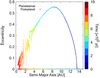Fig. 1

Orbital evolution of a planetesimal initially located at 13.8 AU dictated via the gravitational interaction with a migrating Jupiter-mass protoplanet. The dots and crosses show the locations of the planetesimal and the protoplanet, respectively, and are colour-coded according to time. In this simulation the surface density of disk gas is set to that of the minimum-mass solar nebula and aerodynamic gas drag is included. Here, the protoplanet migrates from 15.0 AU with a migration rate of 10⁵ AU yr⁻¹. For the details of the numerical simulation, see Sect. 3.

2 Analytical expression of the accretion sweet spot

2.1 Overview of planetesimal accretion during planetary migration

Mean motion resonances play an important role in the accretion of planetesimals onto a migrating protoplanet. Here we summarise the orbital evolution of planetesimals dictated via their gravitational interaction with a migrating protoplanet, which was found by the numerical simulations of Shibata et al. (2020). Figure 1 shows the orbital evolution of a planetesimal initially located at 13.8 AU around a migrating Jupiter-mass protoplanet. The orbital evolution of the planetesimal is divided into three characteristic phases as discussed below.

In the first phase (t = 0 yr–4 × 10⁵ yr; blue symbols) the planetesimal encounters the migrating protoplanet and is trapped in the 2:1 mean motion resonance; this phenomenon is referred to as resonant trapping. The planetesimal trapped in a mean motion resonance is transported inward together with the migrating protoplanet and its eccentricity is highly enhanced. This phenomenon is known as resonant shepherding (Batygin & Laughlin 2015).

In the second phase (t = 4 × 10⁵ yr–7 × 10⁵ yr; green–yellow symbols), as time progresses, the resonantly trapped planetesimal starts to escape from the mean motion resonance, and its eccentricity begins to decrease because of the stronger aerodynamic drag in the inner regions. The break of resonant trapping shown in Fig. 1 is caused by overstable libration (Goldreich & Schlichting 2014). The eccentricity of the trapped planetesimal is excited through gravitational scattering by the migrating protoplanet, but is also damped by the disk gas drag. This overstable equilibrium condition makes the planetesimal orbit unstable and breaks the resonant trapping.

In the third phase (t = 7 × 10⁵ yr; red symbols), in the farther inner region, the disk gas is dense enough that the resonantly-trapped planetesimal is damped faster than the planetary migration, and therefore the planetesimal is eliminated from the feeding zone. We refer to this phenomenon as aerodynamic shepherding, which was found by Tanaka & Ida (1999) in the context of terrestrial planet formation.

According to the numerical simulations preformed in Shibata et al. (2020), planetesimal accretion occurs during the second phase, and the region in which efficient planetesimal accretion occurs is referred to as the SSP. During the first and third phases, planetesimal accretion is negligible. The existence of these three different phases (or regions) is associated with the change in strength of the aerodynamic gas drag which increases as the protoplanet migrates inward.

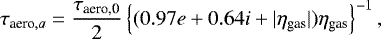
In the following sections, we derive the conditions for the SSP analytically. In Sect. 2.2, we show that planetesimals are generally trapped in mean motion resonances with an approaching protoplanet in standard protoplanetary disks. In Sect. 2.3, we show that the eccentricity of the resonantly trapped planetesimal reaches an equilibrium value, e_eq, that is determined by the ratio of the aerodynamic damping timescale (or the friction timescale) for the planetesimal (τ_{aero, 0}; Eq. (16)) to the tidal damping timescale (or the migration timescale) of the protoplanet (τ_tide,a). A necessary condition for a planetesimal to be captured is that it enters the feeding zone of the protoplanet. As for the resonantly trapped planetesimal, e_eq must exceed the eccentricity at the feeding zone boundary (e_cross; Eq. (27)), which is derived in Sect. 2.4. Even if this condition is satisfied, for the trapped planetesimal to escape the resonance completely the perturbed planetesimal’s orbit must oscillate more widely relative to the resonant width (i.e. the overstable libration), and this oscillation must be amplified more rapidly than the protoplanet’s migration. The conditions are derived in Sect. 2.5. Finally, by putting everything above together, we infer the condition for the SSP in Sect. 2.6.

2.2 Before resonant trapping

When the radial distance between two objects decreases, which is referred to as convergent orbital evolution, the objects are eventually locked in a resonant state. Resonant trapping has been discussed in the contexts of the formation of satellite pairs (e.g. Goldreich 1965; Dermott et al. 1988; Malhotra 1993b), the transport of small bodies (e.g. Yu & Tremaine 2001; Batygin & Laughlin 2015), and the formation of exoplanet pairs (e.g. Fabrycky et al. 2014; Goldreich & Schlichting 2014; Batygin 2015, and references therein). However, not all resonant encounters result in resonant trapping. Resonant trapping requires the following conditions for a planetesimal-protoplanet pair (e.g. Malhotra 1993a):

(i)
The two orbits converge with each other;
(ii)
The eccentricity of the planetesimal, e, before it is trapped in the resonance is smaller than the critical value, e_crit (see Eq. (2));
(iii)
The timescale for the planetesimal to cross the resonant width, τ_cross, is longer than the libration timescale, τ_lib (see Eqs. (3) and (8)).

Here, we consider a trap of a planetesimal in the inner first-order mean motion resonances (j : j − 1 resonance) with a protoplanet migrating inward, and we assume the mass of the planetesimal is negligibly small relative to that of the protoplanet.

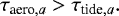
The first condition can be obtained by comparing the timescales of change in the semi-major axis of the planetesimal and the protoplanet. In a protoplanetary gaseous disk the orbits of objects shrink by the aerodynamic gas drag and gravitational tidal drag from the disk gas. The former is dominant for planetesimal-size objects (≲ 10²⁴ g) and the latter is for planet-size objects (≳10²⁴ g) (Zhou & Lin 2007). Using the aerodynamic damping timescale for semi-major axis τ_aero,a for the planetesimal and the tidal damping timescale for semi-major axis τ_tide,a for the protoplanet, we can write the first condition as $τ_{aero, a} > τ_{tide, a} .$ $\begin{align*} \tau_{\textrm{aero},a} > \tau_{\textrm{tide},a}.\end{align*}$ (1)

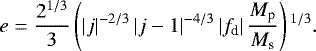
For the second condition, the critical eccentricity for the j : j − 1 resonances is given by (e.g. Murray & Dermott 1999) $e_{crit} = \sqrt{6} {[\frac{3}{| f_{d} |} {(j - 1)}^{4 / 3} j^{2 / 3} \frac{M_{s}}{M_{p}}]}^{- 1 / 3},$ $\begin{align*} e_{\textrm{crit}} = \sqrt{6} \left[ \frac{3}{|f_{\textrm{d}}|} \left(j-1\right){}^{4/3} j^{2/3} \frac{M_{\textrm{s}}}{M_{\textrm{p}}} \right]^{-1/3},\end{align*}$ (2)

where M_p and M_s are the masses of the planet and central star, respectively, and f_d is the interaction coefficient whose values are summarised in Table 1.

When τ_aero,a ≫ τ_tide,a, the timescale for the planetesimal to cross the resonant width τ_cross is given by 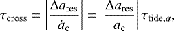$τ_{cross} = | \frac{Δ a_{res}}{{\dot{a}}_{c}} | = | \frac{Δ a_{res}}{a_{c}} | τ_{tide, a},$ $\begin{align*} \tau_{\textrm{cross}} = \left| \frac{\Delta a_{\textrm{res}}}{\dot{a}_{\textrm{c}}} \right| = \left| \frac{\Delta a_{\textrm{res}}}{a_{\textrm{c}}} \right| \tau_{\textrm{tide},a},\end{align*}$ (3)

where a_c is the semi-major axis of the resonance centre, which is related to the protoplanet’s semi-major axis a_p as $a_{c} = {(\frac{j - 1}{j})}^{2 / 3} a_{p};$ $\begin{align*} a_{\textrm{c}} = \left(\frac{j-1}{j}\right){}^{2/3} a_{\textrm{p}};\end{align*}$ (4)

ȧ_c is the temporal change of a_c; and Δa_res is the width of the resonance given by (e.g. Murray & Dermott 1999) $\frac{Δ a_{res}}{a_{c}} = 2 {\frac{16}{3} \frac{M_{p}}{M_{s}} {(\frac{j - 1}{j})}^{2 / 3} e | f_{d} |}^{1 / 2} {1 + \frac{1}{27 {(j - 1)}^{2} e^{3}} \frac{M_{p}}{M_{s}} {(\frac{j - 1}{j})}^{2 / 3} | f_{d} |}^{1 / 2} .$ $\begin{equation*} \frac{\Delta a_{\textrm{res}}}{a_{\textrm{c}}} = 2 \left\{ \frac{16}{3} \frac{M_{\textrm{p}}}{M_{\textrm{s}}} \left(\frac{j-1}{j} \right){}^{2/3} e \left|f_{\textrm{d}} \right| \right\}^{1/2} \\ \left\{ 1+\frac{1}{27 (j-1){}^2 e^3} \frac{M_{\textrm{p}}}{M_{\textrm{s}}} \left(\frac{j-1}{j} \right){}^{2/3} \left| f_{\textrm{d}} \right| \right\}^{1/2}. \end{equation*}$ (5)

The width of the resonance depends on the eccentricity and takes the minimum value at $e = \frac{2^{1 / 3}}{3} {({| j |}^{- 2 / 3} {| j - 1 |}^{- 4 / 3} | f_{d} | \frac{M_{p}}{M_{s}})}^{1 / 3} .$ $\begin{align*} e = \frac{2^{1/3}}{3} \left(\left|j \right|^{-2/3} \left|j-1\right|^{-4/3} \left| f_{\textrm{d}} \right| \frac{M_{\textrm{p}}}{M_{\textrm{s}}} \right){}^{1/3}.\end{align*}$ (6)

By substituting Eq. (6) into Eq. (5), we obtain the minimum width of the resonance as ${\frac{Δ a_{res}}{a_{c}} |}_{min} = \frac{2^{8 / 3}}{3^{1 / 2}} j^{- 4 / 9} {(j - 1)}^{1 / 9} | f_{d} |^{2 / 3} {(\frac{M_{p}}{M_{s}})}^{2 / 3} .$ $\begin{align*} \left. \frac{\Delta a_{\textrm{res}}}{a_{\textrm{c}}} \right|_{\textrm{min}} = \frac{2^{8/3}}{3^{1/2}} j^{-4/9} (j-1){}^{1/9} {|f_{\textrm{d}}|}^{2/3} \left(\frac{M_{\textrm{p}}}{M_{\textrm{s}}} \right){}^{2/3}.\end{align*}$ (7)

The libration timescale at internal resonances is given by (e.g. Murray & Dermott 1999; Batygin & Laughlin 2015) $τ_{lib} = \frac{2 π}{n} | {(\frac{j - 1}{j})}^{4 / 3} {(\frac{M_{p}}{M_{s}})}^{2} \frac{f_{d}^{2}}{e^{2}} {- 3 {(j - 1)}^{2} {(\frac{j - 1}{j})}^{2 / 3} \frac{M_{p}}{M_{s}} f_{d} e |}^{- 1 / 2},$ $\begin{equation*} \tau_{\textrm{lib}} = \frac{2 \pi}{n} \left| \left(\frac{j-1}{j} \right){}^{4/3} \left(\frac{M_{\textrm{p}}}{M_{\textrm{s}}} \right){}^2 \frac{{f_{\textrm{d}}}^2 }{e^2} \right. \\ \left. - 3 (j-1){}^2 \left(\frac{j-1}{j} \right){}^{2/3} \frac{M_{\textrm{p}}}{M_{\textrm{s}}} f_{\textrm{d}} e \right|^{-1/2}, \end{equation*}$ (8)

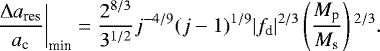
where n is the planetesimal mean motion. Substituting Eq. (6) into Eq. (8), we obtain the corresponding libration timescale as $τ_{lib} = 0.48 j^{4 / 9} {(j - 1)}^{- 10 / 9} {(\frac{M_{p}}{M_{s}})}^{- 2 / 3} | f_{d} |^{- 2 / 3} T_{K},$ $\begin{align*} \tau_{\textrm{lib}} = 0.48 j^{4/9} (j-1){}^{-10/9} \left(\frac{M_{\textrm{p}}}{M_{\textrm{s}}} \right){}^{-2/3} |f_{\textrm{d}}|^{-2/3} T_{\textrm{K}}, \end{align*}$ (9)

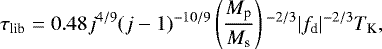
where T_K (= 2π∕n) is the Kepler period at the resonance centre. Using Eqs. (3), (7), and (9), we obtain the third (sufficient) condition as $\frac{τ_{cross}}{τ_{lib}} = 7.7 j^{1 / 9} {(j - 1)}^{2 / 9} | f_{d} |^{4 / 3} {(\frac{M_{p}}{M_{s}})}^{4 / 3} \frac{τ_{tide, a}}{T_{K, p}} ≳ 1,$ $\begin{align*} \frac{\tau_{\textrm{cross}}}{\tau_{\textrm{lib}}} = 7.7 j^{1/9} \left(j-1\right){}^{2/9} |f_{\textrm{d}}|^{4/3} \left(\frac{M_{\textrm{p}}}{M_{\textrm{s}}}\right){}^{4/3} \frac{\tau_{\textrm{tide},a}}{T_{\textrm{K,p}}} \gtrsim 1,\end{align*}$ (10)

where T_K,p is the Kepler period of the migrating protoplanet, specifically T_{K, p} = T_K j∕(j − 1).

Far from the protoplanet and outside mean motion resonances, the planetesimal’s eccentricity is determined by the balance between the viscous stirring from the planetesimal swarm and the aerodynamic gas drag. The mean value of r.m.s. eccentricities of the planetesimal swarm is of the order of ≲ 10⁻² (Ohtsuki et al. 2002). For kilometre-size planetesimals with e = 10⁻², the radial drift timescale τ_damp,a is longer than the planetary migration timescale in the type II regime (τ_tide,a ≲ 10⁷ yr) over a wide region of a protoplanetary disk (Adachi et al. 1976). In addition, the critical eccentricity is e_crit ~ 0.15 for j = 2 and M_p ∕M_s = 10⁻³. Thus, the first and second conditions are expected to be achieved in protoplanetary disks. Figure 2 shows the timescales ratio τ_cross∕τ_lib as a function of semi-major axis, calculated from Eq. (10). Here, we show the cases of 2 : 1 (thick lines) and 3 : 2 (thin lines) resonances, and consider the type II regime for the migration timescale τ_tide,a obtained in Kanagawa et al. (2018). To calculate τ_tide,a, we adopt the self-similar solution of Lynden-Bell & Pringle (1974) for the disk structure with a disk accretion rate of 10⁻⁸ M_⊙ yr⁻¹ and viscosity of 10⁻³. The disk aspect ratio is set to 0.03r^1∕4. The timescales ratio τ_cross∕τ_lib is higher than unity except for the cases of M_p∕M_s = 10⁻⁴ in outer disk a ≫ 10 AU. Thus, we conclude that the resonant trapping of planetesimals usually occurs during the migration of a giant protoplanet.

Table 1

Values of the secular term f_s and the directterm f_d for the first-order mean motion resonances.

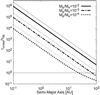Fig. 2

Ratio of the crossing timescale τ_cross (Eq. (3)) to the libration timescale τ_lib (Eq. (9)) as a function of the planetesimal’s semi-major axis. Here, the type II regime obtained in Kanagawa et al. (2018) is considered for the migration timescale τ_tide,a. The solid, dash-dotted, and dotted lines show the cases of the planet-to-star mass ratio M_p ∕M_s= 10⁻², 10⁻³, and 10⁻⁴, respectively. Shown are the inner first-order mean motion resonances (or j:j − 1 resonances): thick lines are for j = 2 and thin lines are for j = 3. To calculate the migration timescale, the same disk model was used as in Ida et al. (2018). The disk accretion rate, disk viscosity parameter, and disk aspect ratio is set to 10⁻⁸ M_⊙ yr⁻¹, 10⁻³, and 0.03r^1∕4, respectively.

2.3 Orbital evolution under resonant trapping

Trapped planetesimals suffer from gravitational perturbation from the migrating protoplanet and aerodynamic gas drag from the disk gas. Lagrange’s equations under the aerodynamic gas drag are given by (e.g. Murray & Dermott 1999) $\dot{a} = 2 (j - 1) C_{r} a e \sin φ - \frac{a}{τ_{aero, a}},$ $\begin{align*} \dot{a} = 2 (j-1) C_{\textrm{r}} a e \sin \varphi -\frac{a}{\tau_{\textrm{aero},a}},\end{align*}$ (11) $\dot{e} = - C_{r} \sin φ - \frac{e}{τ_{aero, e}},$ $\begin{align*} \dot{e} = - C_{\textrm{r}} \sin \varphi -\frac{e}{\tau_{\textrm{aero},e}},\end{align*}$ (12)

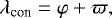
where φ is the resonant angle; 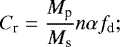$C_{r} = \frac{M_{p}}{M_{s}} n α f_{d};$ $\begin{align*} C_{\textrm{r}} = \frac{M_{\textrm{p}}}{M_{\textrm{s}}} n \alpha f_{\textrm{d}};\end{align*}$ (13)

and τ_aero,a and τ_aero,e are the aerodynamic damping timescales for semi-major axis and eccentricity, which are given by (Adachi et al. 1976) $τ_{aero, a} = \frac{τ_{aero, 0}}{2} {(0.97 e + 0.64 i + | η_{gas} |) η_{gas}}^{- 1},$ $\begin{align*} \tau_{\textrm{aero},a} = \frac{\tau_{\textrm{aero,0}}}{2} \left\{ (0.97 e +0.64 i + |\eta_{\textrm{gas}}|)\eta_{\textrm{gas}} \right\}^{-1},\end{align*}$ (14) $τ_{aero, e} = τ_{aero, 0} {(0.77 e + 0.64 i + 1.5 | η_{gas} |)}^{- 1},$ $\begin{align*} \tau_{\textrm{aero},e} = \tau_{\textrm{aero,0}} \left(0.77 e +0.64 i +1.5|\eta_{\textrm{gas}}| \right){}^{-1},\end{align*}$ (15)

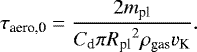where $τ_{aero, 0} = \frac{2 m_{pl}}{C_{d} π R_{pl}^{2} ρ_{gas} v_{K}} .$ $\begin{align*} \tau_{\textrm{aero,0}} = \frac{2 m_{\textrm{pl}}}{C_{\textrm{d}} \pi {R_{\textrm{pl}}}^2 \rho_{\textrm{gas}} v_{\textrm{K}}}.\end{align*}$ (16)

Here C_d is the non-dimensional drag coefficient, m_pl is the planetesimal’s mass, R_pl is the planetesimal’s radius, ρ_gas is the gas density, and v_K is the Kepler velocity. The planetesimal’s mass m_pl is calculated as $4 π ρ_{pl} R_{pl}^{3} / 3$ $4\pi\rho_{\textrm{pl}}{R_{\textrm{pl}}}^3/3$ , where ρ_pl is the planetesimal’s mean density and η_gas is a parameter that defines the sub-Keplerian velocity of disk gas as 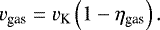$v_{gas} = v_{K} (1 - η_{gas}) .$ $\begin{equation*}v_{\textrm{gas}} = v_{\textrm{K}} \left(1- \eta_{\textrm{gas}} \right). \end{equation*}$ (17)

We note that we have neglected the high-order terms in eccentricity in Eqs. (11), (12), (14), and (15). Although the eccentricities of the trapped planetesimals are easily excited to e² ~ 0.1, the location of the sweet spot analytically derived with these equations is found to be consistent with the numerical results, as shown in Sect. 3.

During the resonant trapping, the period ratio of the protoplanet to the trapped planetesimal remains constant, by definition, and $\frac{a}{\dot{a}} = \frac{a_{p}}{\dot{a_{p}}} = - τ_{tide, a} .$ $\begin{equation*} \frac{a}{\dot{a}} = \frac{a_{\textrm{p}}}{\dot{a_{\textrm{p}}}} = -\tau_{\textrm{tide},a}.\end{equation*}$ (18)

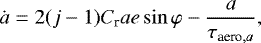
When τ_aero,a ≫ τ_tide,a, using Eq. (18), we can re-write Eq. (11) as $\sin φ = - \frac{1}{2 (j - 1) C_{r} e τ_{tide, a}},$ $\begin{equation*} \sin \varphi = -\frac{1}{2(j-1) C_{\textrm{r}} e \tau_{\textrm{tide},a}},\end{equation*}$ (19)

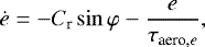
and using Eq. (19) in Eq. (12) we obtain $\dot{e} = \frac{1}{2 (j - 1) e τ_{tide, a}} - \frac{e}{τ_{aero, e}} .$ $\begin{equation*} \dot{e} = \frac{1}{2(j-1)e \tau_{\textrm{tide},a}} -\frac{e}{\tau_{\textrm{aero},e}}.\end{equation*}$ (20)

Just after being trapped in the resonances, e is small and ė is positive. Equation (20) indicates that e increases on a timescale ~e² τ_tide,a (≪ τ_tide,a) and reaches an equilibrium value. Solving Eqs. (19) and (20) with ė = 0, we obtain the equilibrium eccentricity and resonant argument given by $e_{eq} = {\frac{1}{2 (j - 1)} \frac{τ_{aero, e}}{τ_{tide, a}}}^{1 / 2},$ $\begin{align*} e_{\textrm{eq}} = \left\{ \frac{1}{2(j-1)} \frac{\tau_{\textrm{aero},e}}{\tau_{\textrm{tide},a}} \right\}^{1/2},\end{align*}$ (21) $\sin φ_{eq} = - \frac{e_{eq}}{C_{r} τ_{aero, e}} .$ $\begin{align*} \sin \varphi_{\textrm{eq}} = - \frac{e_{\textrm{eq}}}{C_{\textrm{r}} \tau_{\textrm{aero},e}}.\end{align*}$ (22)

Unlike the eccentricity, the planetesimals’ inclinations are not excited by the migrating protoplanet because the planetesimals are far from the protoplanet. When e ≫ i and e ≫ η_gas, $τ_{aero, e} = τ_{aero, 0} {(0.77 e)}^{- 1}$ $\tau_{\mathrm{aero},e} = \tau_{\textrm{aero,0}} (0.77 \textrm{e}){}^{-1}$ from Eq. (15), and thus e_eq and sinφ_eq are written approximately as $e_{eq} ~ {\frac{1}{1.54 (j - 1)} \frac{τ_{aero, 0}}{τ_{tide, a}}}^{1 / 3},$ $\begin{align*} e_{\textrm{eq}} \sim \left\{ \frac{1}{1.54 (j-1)} \frac{\tau_{\textrm{aero,0}}}{\tau_{\textrm{tide},a}} \right\}^{1/3},\end{align*}$ (23) $\sin φ_{eq} ~ - \frac{0.77 e_{eq}^{2}}{C_{r} τ_{aero, 0}} .$ $\begin{align*} \sin \varphi_{\textrm{eq}} \sim -\frac{0.77{e_{\textrm{eq}}}^2}{C_{\textrm{r}} \tau_{\textrm{aero,0}}}.\end{align*}$ (24)

We note that if the high-order terms of the eccentricity are considered, the equilibrium eccentricity is smaller than that given by Eq. (23).

2.4 Aerodynamic shepherding

As shown in Shibata et al. (2020), mean motion resonances play a role like narrow flow channels for planetesimals to enter the planet’s feeding zone; the channels are called the accretion bands. Mathematically speaking, planetesimals with negative values of the Jacobi energy, E_Jacobi, can enter the feeding zone once their eccentricities are sufficiently enhanced so that their Jacobi energy becomes positive. The Jacobi energy is given by (Hayashi et al. 1977) $E_{Jacobi} = \frac{G M_{s}}{a_{p}} {- \frac{a_{p}}{2 a} - \sqrt{\frac{a}{a_{p}} (1 - e^{2})} \cos i + \frac{3}{2} + \frac{9}{2} h^{2} + O (h^{3})} ,$ $\begin{align*}E_{\textrm{Jacobi}} = \frac{\mathcal{G} M_{\textrm{s}}}{a_{\textrm{p}}} \!\left\{ -\frac{a_{\textrm{p}}}{2 a} - \!\sqrt{\frac{a}{a_{\textrm{p}}} \left(1-\textrm{e}^2\right)} \cos {i} + \frac{3}{2} + \frac{9}{2} h^2 +O(h^3) \right\}\!, \end{align*}$ (25)

where h is the reduced Hill radius defined as $h = {(\frac{M_{p}}{3 M_{s}})}^{1 / 3} .$ $\begin{align*}h = \left(\frac{M_{\textrm{p}}}{3 M_{\textrm{s}}} \right){}^{1/3}. \end{align*}$ (26)

Substituting E_jacobi = 0 and 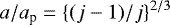$a / a_{p} = {(j - 1) / j}^{2 / 3}$ $a/a_{\textrm{p}} = \left\{(j-1)/j\right\}^{2/3}$ into Eq. (25) and assuming cos²i ~ 1, we obtain the eccentricity of the accretion band, e_cross: $e_{cross} = {[1 - {(\frac{j}{j - 1})}^{2 / 3} {\frac{3}{2} + \frac{9}{2} h^{2} - \frac{1}{2} {(\frac{j}{j - 1})}^{2 / 3}}^{2}]}^{1 / 2} .$ $\begin{align*} e_{\textrm{cross}} = \left[ 1- \left(\frac{j}{j-1} \right){}^{2/3} \left\{ \frac{3}{2} +\frac{9}{2} h^2 -\frac{1}{2} \left(\frac{j}{j-1} \right){}^{2/3} \right\}^2 \right]^{1/2}.\end{align*}$ (27)

The condition required for entering the feeding zone is that the equilibrium eccentricity, e_eq (see Eq. (23)), is larger than e_cross, which is given by $1.54 (j - 1) e_{cross}^{3} < \frac{τ_{aero, 0}}{τ_{tide, a}} .$ $\begin{align*} 1.54 (j-1) {e_{\textrm{cross}}}^3 < \frac{\tau_{\textrm{aero,0}}}{\tau_{\textrm{tide},a}}.\end{align*}$ (28)

Figure 3 shows e_cross as a function of M_p∕M_s for different values of j from Eq. (27). As indicated in this figure, e_cross decreases with increasing planetary mass; as the protoplanet mass increases, the feeding zone expands, and consequently the crossing point itself (i.e. the accretion band) is located inside the feeding zone once the planetary mass exceeds a certain value. For example, there are three crossing points (j = 2, 3, 4) when M_p ∕M_s = 10^−3.5, but there is only one crossing point (j = 2) when M_p∕M_s = 10^−2.5 and no points when M_p∕M_s = 10⁻².

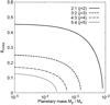Fig. 3

Dependence of the crossing point eccentricity e_cross (see Eq. (27)) on the planet-to-star mass ratio M_p∕M_s for four different cases: j = 2 (solid), j = 3 (dashed), j = 4 (dash-dotted), and j = 5 (dotted).

2.5 Resonant breaking

Even when entering the feeding zone, planetesimals trapped in mean motion resonances are not always accreted by the migrating protoplanet.The conjunction point of a trapped planetesimal with the protoplanet is given in terms of the mean longitude as $λ_{con} = φ + ϖ,$ $\begin{align*} \lambda_{\textrm{con}} = \varphi + \varpi, \end{align*}$ (29)

where ϖ is the longitude of pericenter. The resonant argument, φ, which is the displacement of the longitude of conjunction from the pericenter, takes φ_eq~ 0 during the converging orbital evolution. This means that every conjunction occurs at the pericenter of the planetesimal orbit; specifically, the planetesimal’s orbit is far from the protoplanet’s at the conjunction. Thus, trapped planetesimals cannot enter the Hill sphere of the protoplanet and planetesimal accretion does not occur (see Figs. C.1 and C.2 in Shibata et al. 2020).

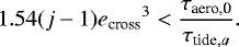
A planetesimal is captured by the migrating protoplanet only if the resonant trapping is broken. Under the forces damping and enhancing the planetesimal’s eccentricity, the orbit of the trapped planetesimal becomes unstable and starts to oscillate. Once the amplitude of oscillation exceeds the resonant width, the resonant trapping is broken. This phenomenon is called the overstable libration and Goldreich & Schlichting (2014) derived the condition required for the instability to grow. Substituting Eqs. (15) and (23) into Eq. (28) of Goldreich & Schlichting (2014), we obtain the breaking condition for resonant trapping due to overstable libration under the aerodynamic gas drag as $3.29 {(\frac{j}{j - 1})}^{3 / 2} \frac{M_{p}}{M_{s}} < \frac{τ_{aero, 0}}{τ_{tide, a}} .$ $\begin{align*} 3.29 \left(\frac{j}{j-1}\right){}^{3/2} \frac{M_{\textrm{p}}}{M_{\textrm{s}}} < \frac{\tau_{\textrm{aero,0}}}{\tau_{\textrm{tide},a}}.\end{align*}$ (30)

Even when this condition is satisfied it takes a time of ~ τ_aero,e for the instability to grow (Goldreich & Schlichting 2014). If τ_aero,e > τ_tide,a, the trapped planetesimal is shepherded into the inner disk before escaping the resonance. The second condition required for the overstable libration is τ_aero,e < τ_tide,a, which we can write as $\frac{τ_{aero, 0}}{τ_{tide, a}} < 0.54 {(j - 1)}^{- 1 / 2},$ $\begin{align*} \frac{\tau_{\textrm{aero,0}}}{\tau_{\textrm{tide},a}} < 0.54 (j-1){}^{-1/2},\end{align*}$ (31)

using Eqs. (15) and (23).

2.6 Required condition for the accretion sweet spot

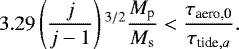
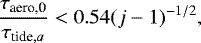
The required condition for the SSP is summarised as 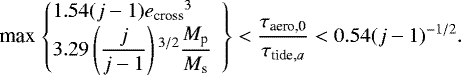$max {\begin{array}{l} 1.54 (j - 1) e_{cross}^{3} \\ 3.29 {(\frac{j}{j - 1})}^{3 / 2} \frac{M_{p}}{M_{s}} \end{array}} < \frac{τ_{aero, 0}}{τ_{tide, a}} < 0.54 {(j - 1)}^{- 1 / 2} .$ $\begin{align*} \textrm{max} \left. \begin{cases} 1.54 (j-1) {e_{\textrm{cross}}}^3\\ \displaystyle{ 3.29 \left(\frac{j}{j-1}\right){}^{3/2} \frac{M_{\textrm{p}}}{M_{\textrm{s}}}\!\!\!\! } \end{cases} \right\} < \frac{\tau_{\textrm{aero,0}}}{\tau_{\textrm{tide},a}} < 0.54 (j-1){}^{-1/2}. \end{align*}$ (32)

The inner edge of the SSP is regulated by the aerodynamic shepherding and resonant shepherding. The dominating process depends on the planetary mass. On the other hand, the outer edge of SSP is regulated by the resonant shepherding alone.

To derive these equations, we assume that τ_aero,a ≫ τ_tide,a. Using the equilibrium eccentricity, we transform this condition as 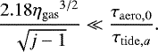$\frac{2.18 η_{gas}^{3 / 2}}{\sqrt{j - 1}} ≪ \frac{τ_{aero, 0}}{τ_{tide, a}} .$ $\begin{align*} \frac{2.18 {\eta_{\textrm{gas}}}^{3/2}}{\sqrt{j-1}} \ll \frac{\tau_{\mathrm{aero},0}}{\tau_{\mathrm{tide},a}}. \end{align*}$ (33)

In the nominal disk model, η_gas is of the order of 10⁻³, and this condition is easily achieved in the SSP. Thus, Eq. (32) can be used for small planetesimals as long as the gas drag strength is scaled by Eq. (16). We find that the location of the SSP is determined by the ratio of the gas drag damping timescale, τ_aero,0, to the planetary migration timescale, τ_tide,a. We therefore conclude that our theoretical prediction is robust (and rather general) since the derivation of this condition does not depend on the assumed disk and migration models. As a result, Eq. (32) can be generally applied to various models of planetesimal accretion.

3 Comparison with numerical results

In this section we validate the derived equation for the SSP by comparison with numerical results. To this end, we perform N-body simulations similar to those presented in Shibata et al. (2020). We adopt different values of model parameters from those in Shibata et al. (2020) in order to identify whether the SSP is indeed regulated by the ratio of the two timescales, τ_aero,0 and τ_tide,a.

3.1 Numerical model and settings

We considerthe following scenario. Gas accretion has terminated and the young giant planet no longer grows in mass. The planet then migrates radially inward from a given semi-major axis within a protoplanetary disk. Initially there are many equal-sized planetesimals interior to the planet’s orbit. The migrating planet then encounters these planetesimals and captures some of them. The planetesimals are represented by test particles, and therefore are affected only by the gravitational forces from the central star and planet, and the drag force by the disk gas. Here, we summarise our numerical model. The details of our numerical model are described in Appendix A.

We assume that the planetary migration timescale is given by $τ_{tide, a} = τ_{tide, 0} {(\frac{a_{p}}{1 AU})}^{1 / 2},$ $\begin{align*} \tau_{\textrm{tide},a} = \tau_{\textrm{tide,0}} \left(\frac{a_{\textrm{p}}}{1 \;\textrm{AU}} \right){}^{1/2},\end{align*}$ (34)

where τ_tide,0 is a scaling parameter. For the drag force by the disk gas, we adopt a model by Adachi et al. (1976). The gas drag force depends on the size of planetesimal R_pl and the profile of ambient disk gas. To focus on the dynamic process, we adopt simply the minimum-mass solar nebula model (Hayashi 1981) as our gas disk model. The surface density, Σ_gas, and the disk temperature, T_disk, are given by $Σ_{gas} = Σ_{gas, 0} {(\frac{r}{1 AU})}^{- α_{disk}},$ $\begin{align*} \Sigma_{\textrm{gas}} = \Sigma_{\textrm{gas,0}} \left(\frac{r}{1\;\textrm{AU}} \right){}^{-\alpha_{\textrm{disk}}},\end{align*}$ (35) $T_{disk} = T_{disk, 0} {(\frac{r}{1 AU})}^{- 2 β_{disk}},$ $\begin{align*} T_{\textrm{disk}} = T_{\textrm{disk,0}} \left(\frac{r}{1\;\textrm{AU}} \right){}^{-2\beta_{\textrm{disk}}},\end{align*}$ (36)

where r is the radial distance from the initial mass centre of the star-planet system, Σ_gas,0 = 1.7 × 10³ g cm⁻², α_disk = 3∕2, T_disk,0 = 280 K, and β_disk = 1∕4. The protoplanetary disk is assumed to be vertically isothermal.

For the planetesimals we adopt a simple surface density profile given by $Σ_{solid} = Z_{s} Σ_{gas, 0} {(\frac{r}{1 AU})}^{- α_{disk}^{'}},$ $\begin{align*} \Sigma_{\textrm{solid}} = Z_{\textrm{s}} \Sigma_{\textrm{gas,0}} \left(\frac{r}{1\;\textrm{AU}} \right){}^{-\alpha_{\textrm{disk}}^{\prime}},\end{align*}$ (37)

where Z_s is the solid-to-gas ratio (or the metallicity) and $α_{disk}^{'} = α_{disk} = 3 / 2$ $\alpha_{\textrm{disk}}^{\prime}=\alpha_{\textrm{disk}}=3/2$ . To speed up the numerical integration, we follow the orbital motion of super-particles, each of which contains several equal-sized planetesimals. The super-particles are initially distributed in a_pl,in < r < a_pl,out with a_pl,in = 0.3 AU and a_pl,out = 20 AU. The planet is initially located in such a way that the inner boundary of the feeding zone is consistent with the outer edge of the planetesimals disk: $a_{p, 0} = \frac{a_{pl, out}}{1 - 2 \sqrt{3} h} .$ $\begin{align*} a_{\textrm{p,0}} = \frac{a_{\textrm{pl,out}}}{1-2\sqrt{3} h}.\end{align*}$ (38)

The calculation is artificially stopped once the planet reaches the orbit of a_p,f= 0.5 AU. First, we investigate the planetesimal accretion in a reference case, where τ_tide,0 = 1 × 10⁵ yr, R_pl= 1 × 10⁷ cm, and M_p= 1 × 10⁻³M_s. In the reference case the total number of planetesimals is M_tot ~ 43 M_⊕. The choices of the parameter values for the reference model are summarised in Table 2. We perform a parameter study for various values of τ_tide,0, R_pl, and M_p. The dynamical integration for the planetesimals is performed using the numerical simulation code developed by Shibata & Ikoma (2019). In this code we integrate the equation of motion using the forth-order Hermite integration scheme (Makino & Aarseth 1992). For the timesteps we adopt the method of Aarseth (1985).

Table 2

Parameters used in the reference model.

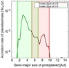Fig. 4

Planetesimal accretion rate vs. the semi-major axis of the migrating planet. The vertical solid lines showthe boundaries of the SSP given by Eq. (32). The red lines are for the case of j = 2 and the green lines are for j = 3. The filled areas show the SSP.

3.2 Comparison with the numerical result

Figure 4 shows the planetesimal accretion rate at each semi-major axis of the migrating protoplanet, obtained in the simulation for the reference model. Planetesimal accretion is found to occur efficiently in a region of 2 AU ≲ a_p ≲ 10 AU. Beyond 10 AU, planetesimals are trapped in mean motion resonances of j = 2 and 3 with the migrating protoplanet. Our analysis of the numerical results shows that the condition of overstable libration is achieved, but the timescale of the instability growth is longer than the migration timescale; thus, the trapped planetesimals are shepherded without being captured by the protoplanet. Around ~ 10 AU, planetesimals trapped in the 2:1 mean motion resonance start to escape due to the overstable libration. The large number of shepherded planetesimals are supplied into the planetary feeding zone, so that the accretion rate peaks at around ~ 8 AU. Aerodynamic shepherding starts around 5 AU for the planetesimals in the 2:1 mean motion resonance, halting the supply of planetesimals through the 2:1 mean motion resonance and reducing the accretion rate significantly. Instead, planetesimal supply resumes through the 3:2 mean motion resonance around 7 AU and the accretion rate increases again. More specifically, planetesimals that remain to be brought into the feeding zonethrough 2:1 mean motion resonance move to the 3:2 resonance (i.e. the accretion band shifts from j = 2 to j = 3). The accretion rate peaks again around 3 AU and then rapidly decreases around 2 AU due to aerodynamic shepherding.

In the simulation setting the timescales ratio is given by $\frac{τ_{aero, 0}}{τ_{tide, a}} = {| \frac{τ_{aero, 0}}{τ_{tide, a}} |}_{1 AU} {(\frac{j - 1}{j})}^{1 / 3} a^{11 / 4},$ $\begin{align*} \frac{\tau_{\textrm{aero,0}}}{\tau_{\textrm{tide},a}} = \left| \frac{\tau_{\textrm{aero,0}}}{\tau_{\textrm{tide},a}} \right|_{1 \;\textrm{AU}} \left(\frac{j-1}{j} \right){}^{1/3} a^{11/4},\end{align*}$ (39) $= {| \frac{τ_{aero, 0}}{τ_{tide, a}} |}_{1 AU} {(\frac{j - 1}{j})}^{13 / 6} a_{p}^{11 / 4},$ $\begin{align*} = \left| \frac{\tau_{\textrm{aero,0}}}{\tau_{\textrm{tide},a}} \right|_{1 \;\textrm{AU}} \left(\frac{j-1}{j} \right){}^{13/6} {a_{\textrm{p}}}^{11/4},\end{align*}$ (40)

where ${| \frac{τ_{aero, 0}}{τ_{tide, a}} |}_{1 AU} = 4.2 \times 10^{- 3} (\frac{R_{pl}}{10^{7} cm}) {(\frac{τ_{tide, 0}}{10^{5} yr})}^{- 1} .$ $\begin{align*} \left| \frac{\tau_{\textrm{aero,0}}}{\tau_{\textrm{tide},a}} \right|_{1 \textrm{AU}} = 4.2\,{\times}\,10^{-3} \left(\frac{R_{\textrm{pl}}}{10^7~\textrm{cm}} \right) \left(\frac{\tau_{\textrm{tide,0}}}{10^5~\textrm{yr}} \right){}^{-1}.\end{align*}$ (41)

The red-shaded and green-shaded areas in Fig. 4 show the predicted regions of the SSP, 5 AU ≲ a_p ≲ 10 AU for j = 2 and 1 AU ≲ a_p ≲ 7 AU for j = 3, which are obtained using Eqs. (40) and (41) in Eq. (32). These regions turn out to cover the areas where the accretion rate is higher than 10⁻⁶ M_⊕ yr⁻¹. Thus, we conclude that the derived equation for the SSP reproduces well the numerical results in the reference model.

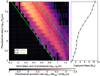Fig. 5

Results of the parameter study regarding the size of planetesimals R_pl. Left: planetesimal accretion rate shown as a colour contour on a plane of the semi-major axis of the migrating protoplanets and the radius of the planetesimals, The analytically predicted inner and outer boundaries of the sweet spot are indicated with solid and dashed lines, respectively. The red lines are for j = 2 and the green lines are for j = 3. Right: total mass of captured planetesimals as a function of the planetesimal radius.

3.3 Results of parameter studies

As seen in Eq. (32), the location of the SSP depends on the ratio of the gas drag damping timescale, τ_aero,0, to the planetary migration timescale, τ_tide,a, and on the planetary mass, M_p. To investigate this dependence, we perform parameter studies for the size of planetesimals, R_pl, which determines τ_aero,0; the scaling factor of migration timescale, τ_tide,0; and the planetary mass, M_p.

3.3.1 Dependence on the planetesimal size

Since the gas drag damping timescale, τ_aero,0, increases with the size of planetesimals, the location of the SSP is predicted to be closer to the central star for larger planetesimals (see e.g. Eqs. (40) and (41)). We perform the numerical simulations, changing the size of planetesimals from 1 × 10⁵ cm to 1 × 10⁸ cm (or ~ 0.01M_⊕). We note that the assumption that mutual gravitational interaction among planetesimals is negligible is not valid for large planetesimals with sizes of R_pl ~ 10⁸ cm. Nevertheless, a study for a wide parameter range is useful to deepen the physical understanding of the effect of the damping timescale onplanetesimal accretion.

Figure 5 shows the results of the parameter study when changing the planetesimal’s radius, R_pl. In the left panel the planetesimal accretion rate is shown as a colour contour on a plane of the semi-major axis of the migrating protoplanet and the planetesimal’s radius. The analytically predicted inner and outer boundaries of the SSP derived in Sect. 2.3 are shown with the solid and dashed lines, respectively. The red lines are for j = 2 and the green lines are for j = 3. In the right panel, the total mass of captured planetesimals M_{cap, tot} is plotted asa function of the planetesimal’s radius.

The location of the SSP (i.e. the region of high accretion rates) is found to be well reproduced by the analytical expressions derived in Sect. 2.3. The maximum accretion rate and the total captured heavy-element mass are higher for larger planetesimals. This occurs because as the SSP moves inward, the number of planetesimals shepherded into the SSP increases. More planetesimals are shepherded into the SSP when the planetesimals are larger, where the SSP locates farther from the initial planet location (or closer to the central star).

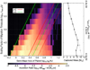Fig. 6

Same as Fig. 5, but for the results of the parameter study regarding the migration timescale τ_tide,0. The grey circles in the right panel show the results of the parameter study regarding the size of planetesimals, R_pl, for comparison using the fraction of timescales τ_aero,0∕τ_tide,a on the vertical axis.

3.3.2 Dependence on the planetary migration timescale

Next, we perform a parameter study when changing the planetary migration timescale. Our analytic consideration above indicates that the location of the SSP is closer to the central star for faster planetary migration. We perform numerical simulations with various migration timescales by changing the scaling factor of the migration timescale, τ_tide,0, from 1 × 10⁴ yr to 1 × 10⁶ yr.

Figure 6 shows the dependence of the results on the migration timescale, τ_tide,0. In the left panel the SSP is found to be closer to the star for faster planetary migration (or smaller τ_tide,0). Since the SSP moves inward as τ_tide,0 decreases, for the same reason described above, the total mass of captured planetesimals, M_{cap, tot}, increases with decreasing τ_tide,0, which is confirmed in the right panel. The right axis shows τ_aero,0∕τ_tide,a at 1 AU calculated with Eq. (41). For comparison, we also plot with grey circles the M_{cap, tot} versus τ_aero,0∕τ_tide,a relation by converting the result shown in the right panel of Fig. 5 when using Eq. (41). Except for τ_tide,0 ≲ 10^4.6 yr, the two results are similar. This confirms that the location of the SSP scales with the ratio of the timescales, τ_aero,0∕τ_tide,a.

The effects of planetary migration, however, seem somewhat more complicated relative to the dependence on the planetesimal’s radius. First, as shown in the left panel, for relatively fast migration (τ_tide,0 ≲ 10^4.6 yr), the outer boundary of the SSP expands beyond the one inferred analytically. Second, the M_{cap, tot} versus τ_aero,0∕τ_tide,a relation differs between the cases when we vary R_pl and varying τ_tide,0 for τ_tide,0 ≲ 10^4.6 yr. This is related to the stability of resonant trapping. As shown in Sect. 2.2, the condition required for resonant trapping is that the timescale for planetesimals to cross the mean motion resonance is longer than the libration timescale. Using Eq. (10) we find that stable resonant trapping is difficult for fast planetary migration like τ_tide,0 ≲ 10⁴ yr.

Figure 7 shows the changes in the phase angle of a planetesimal initially located at a₀ = 13.8 AU in the cases of (a) τ_tide,0 = 10⁴ yr and (b) τ_tide,0 = 10⁵ yr. In panel a, the phase angle continues libration even after trapped into the resonance. This occurs because fast planetary migration perturbs the orbit of the trapped planetesimal and accelerates the overstable libration. The resonant trapping is thus broken earlier in the case of τ_tide,0 = 10⁴ yr than in the case of τ_tide,0 = 10⁵ yr, which results in the outward expansion of the SSP. However, such an outward shift of the outer edge of the SSP does not lead to an increase in the mass of captured planetesimals because fast planetary migration breaks the resonant trapping as soon as the trapped planetesimal reaches the equilibrium condition. The planetesimal in panel a escapes from the resonant trapping with e ~ 0.7 and that in panel b with e ~ 0.4. The capture probability of planetesimals decreases with increasing eccentricity (Ida & Nakazawa 1989); thus, the total mass of captured planetesimals does not increase with the expansion of the SSP in the cases of τ_tide,0 ≲ 10^4.6 yr.

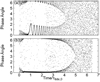Fig. 7

Change in the phase angle of a planetesimal initially located at a₀ = 13.8 AU. Panel a shows the case of τ_tide,0 = 1 × 10⁴ yr and panel b shows the case of τ_tide,0 = 1 × 10⁵ yr. In panel a, the phase angle oscillates indicating that the resonant trapping is unstable due to fast planetary migration. Then, the resonant trapping is broken earlier in the case of panel a than that shown in panel b.

3.3.3 Dependence on the planetary mass

Finally, we perform a parameter study of the simulations when varying the mass of the migrating protoplanet, M_p, in the range of M_p∕M_s between 1 × 10⁻⁴ and 1 × 10⁻². The results are summarised in Fig. 8. We find that the semi-major axis of the outer boundary of the SSP is insensitive to the protoplanet mass, which is consistent with Eq. (32). In this figure, we indicate the locations of the inner edge of the SSP for j = 4 and 5 in addition to those for j = 2 and 3 given by Eq. (32), confirming that Eq. (32) accurately reproduces the numerical result. As shown in Fig. 3, the crossing points between the resonance centre and the feeding zone boundary disappear once the planetary mass exceeds a specific value. In Fig. 8, we show the M_p –a_p relation corresponding to the disappearance of the crossing points with grey solid lines. This is also consistent with the numerical result.

As found in Shibata et al. (2020), the total mass of captured planetesimals M_cap,tot changes with the planetary mass in a non-monotonic manner and takes local maxima at M_p ∕M_s ~ 10^−3.6, 10^−3.3, 10^−2.7, and 10^−2.2. These periodical changes come from the corresponding shifts of the inner boundary of the SSP. The shepherding process that regulates the inner boundary of the SSP changes from the aerodynamic shepherding to the resonant shepherding with increasing planetary mass. The accretion bands also change with the protoplanet mass. Because of these effects the location of the inner boundary of the SSP shifts non-monotonically which results in the non-monotonic change of M_cap,tot. The global decreasing trend with increasing protoplanet mass comes from the outward shift of the inner boundary.

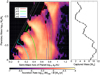Fig. 8

Same as Fig. 5, but for the results of the parameter study when varying the protoplanet’s mass, M_p. The red, green, sky blue, and blue lines represent the SSP inner (solid lines) and outer (dashed lines) boundaries determined by the resonant trapping, which is predicted by Eq. (32) for j = 2, 3, 4, and 5, respectively. The coloured lines change into the grey lines once the protoplanet mass exceeds a threshold value, beyond which the accretion bands disappear (see Fig. 3).

4 Discussion

4.1 Collision and ablation of highly excited planetesimals

Our model neglects the effect of planetesimal collisions. During planetary migration, planetesimals are swept by the resonances, and the enhanced local density of planetesimals increases the frequency of planetesimal collisions, which might initiate a collisional cascade (Batygin & Laughlin 2015). A collisional cascade (e.g. Dohnanyi 1969) changes the size distribution of planetesimals and the perturbation adding on the planetesimal orbits by the collisions would also affect the resonant configuration (Malhotra 1993b). In this section we consider the effect of planetesimal collisions on the location of the SSP and the planetesimal accretion.

4.1.1 Collision timescale of shepherded planetesimals

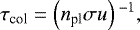
First, we estimate the collision timescale using the number density of planetesimals, n_pl ; the collision cross section, σ; and the relative velocity, u. We considera swarm of planetesimals that is trapped in mean motion resonances with total mass of M_shep. For simplicity, we consider that these planetesimals have the same mass. The planetesimals are distributed in the ring-like region with a width of $~ 2 a < e >$ ${\sim} 2 a\left< e\right>$ and thickness of $~ 2 a \tan $ ${\sim} 2 a \tan \left< i\right>$ . The collision timescale between these planetesimals τ_col is given as $τ_{col} = {(n_{pl} σ u)}^{- 1},$ $\begin{equation*} \tau_{\textrm{col}} = \left(n_{\textrm{pl}} \sigma u \right){}^{-1}, \end{equation*}$ (42) $= (M_{shep} {2 π a \cdot 2 a < e > \cdot 2 a \tan } \cdot π R_{pl}^{2} \cdot < e > v_{K})^{- 1},$ $\begin{equation*} = \left(\frac{M_{\textrm{shep}}}{2 \pi a \cdot 2 a \left<e\right> \cdot 2 a \tan \left<i\right>} \cdot \pi {R_{\textrm{pl}}}^2 \cdot \left< e\right> v_{\textrm{K}} \right){}^{-1}, \end{equation*}$ (43) $= 3 \times 10^{5} yr {(\frac{M_{shep}}{10 M_{\oplus}})}^{- 1} (\frac{ρ_{pl}}{2 g {cm}^{- 3}}) (\frac{R_{pl}}{10^{7} cm}) {(\frac{a}{10 AU})}^{7 / 2} (\tan } 10^{- 3}) {(\frac{M_{s}}{M_{⊙}})}^{- 1 / 2} .$ $\begin{equation*} = 3\,{\times}\,10^5\,\textrm{yr} \left(\frac{{M}_{\textrm{shep}}}{10 \;{M}_{\oplus}} \right){}^{-1} \left(\frac{\rho_{\textrm{pl}}}{2 \,\textrm{g}\,\textrm{cm}^{-3}} \right) \left(\frac{{R}_{\textrm{pl}}}{10^{7}\,\textrm{cm}} \right) \\ \quad \left(\frac{a}{10\,\textrm{AU}} \right){}^{7/2} \left(\frac{\tan \left< i\right>}{10^{-3}} \right) \left(\frac{M_{\textrm{s}}}{M_{\odot}} \right){}^{-1/2}. \end{equation*}$ (44)

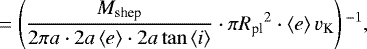
Here we neglect the effect of gravitational focusing because of the high relative velocities of planetesimals. The value of M_shep increases as the protoplanet migrates and sweeps planetesimals, but decreases after reaching the SSP because the trapped planetesimals start to escape from mean motion resonances. As suggested by Eq. (44), τ_col rapidly decreases with the inward planetary migration. Planetesimals start to collide with each other where the collision timescale, τ_col, is comparable to the migration timescale, τ_tide,a. The maximum mass of planetesimals shepherded into the SSP without active planetesimal collisions, M_shep,max, is estimated as $M_{shep, max} = 30 M_{\oplus} {(\frac{τ_{tide, a}}{10^{5} yr})}^{- 1} (\frac{ρ_{pl}}{2 g {cm}^{- 3}}) (\frac{R_{pl}}{10^{7} cm}) {(\frac{a}{10 AU})}^{7 / 2} (\tan } 10^{- 3}) {(\frac{M_{s}}{M_{⊙}})}^{- 1 / 2} .$ $\begin{align*} M_{\textrm{shep,max}} = 30 \;M_{\oplus} \left(\frac{\tau_{\mathrm{tide},a}}{10^5\,\textrm{yr}} \right){}^{-1} \left(\frac{\rho_{\textrm{pl}}}{2 \,\textrm{g}\,\textrm{cm}^{-3}} \right) \left(\frac{R_{\textrm{pl}}}{10^7\,\textrm{cm}} \right) \\ \left(\frac{a}{10 \;\textrm{AU}} \right){}^{7/2} \left(\frac{\tan \left< i\right>}{10^{-3}} \right) \left(\frac{M_{\textrm{s}}}{M_{\odot}} \right){}^{-1/2}. \end{align*}$ (45)

Figure 9 shows M_shep,max as a function of the radial distance from the central star. During the planetary migration, despite the increase in M_shep, M_shep,max rapidly decreases. We conclude that the trapped planetesimals collide with each other during the planetary migration phase if the protoplanet migrates a long distance in the radial direction before entering the SSP.

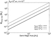Fig. 9

Maximum mass of planetesimals that can be shepherded in mean motion resonances without effective mutual collisions. We show the cases of R_pl = 10⁷ cm and = 10⁻³. The solid, dashed, and dotted lines correspond to τ_tide,a = 10⁶ yr, 10⁵ yr, and 10⁴ yr, respectively.

4.1.2 Collisional acscade in the resonant shepherding

The outcome of planetesimal collision is determined by the specific energy, which is the kinetic energy of impacting planetesimal normalised by the mass of impacted planetesimal, given by (e.g. Armitage 2010) $Q = 1.1 \times 10^{12} erg g^{- 1} {(\frac{e}{0.5})}^{2} {(\frac{R_{im}}{R_{pl}})}^{3} (\frac{M_{s}}{M_{⊙}}) {(\frac{a}{10 AU})}^{- 1},$ $\begin{align*}Q = 1.1\,{\times}\,10^{12} \;\textrm{erg}\;{\textrm{g}}^{-1} \left(\frac{e}{0.5} \right){}^2 \left(\frac{R_{\textrm{im}}}{R_{\textrm{pl}}} \right){}^{3} \left(\frac{M_{\textrm{s}}}{M_{\odot}} \right) \left(\frac{a}{10\,\textrm{AU}} \right){}^{-1}, \end{align*}$ (46)

where R_im is the radius of the impacting planetesimal. The critical value for shattering planetesimals can be scaled as $Q_{D}^{*} = q_{s} {(\frac{R_{pl}}{1 cm})}^{a} + q_{g} ρ_{pl} {(\frac{R_{pl}}{1 cm})}^{b} .$ $\begin{align*} Q_{\textrm{D}}^{*} = q_{\textrm{s}} \left(\frac{R_{\textrm{pl}}}{1 \;\textrm{cm}} \right){}^{a} + q_{\textrm{g}} \rho_{\textrm{pl}} \left(\frac{R_{\textrm{pl}}}{1 \;\textrm{cm}} \right){}^{b}.\end{align*}$ (47)

Benz & Erik (1999) and Leinhardt & Stewart (2009) determined the values of fitting parameters in this equation. For icy planetesimals with an impact velocity of 3 km s⁻¹ they obtained q_s = 1.6 × 10⁷ erg g⁻¹, q_g = 1.2 erg cm³ g⁻², a = −0.39, and b = 1.26. Using Eqs. (46) and (47), we find that kilometre-size planetesimals are shattered by the collisions of planetesimals larger than R_im,th, which is given as $\frac{R_{im, th}}{R_{pl}} = 0.13 {(\frac{R_{pl}}{10^{7} cm})}^{0.42} {(\frac{e}{0.5})}^{- 2 / 3} {(\frac{M_{s}}{M_{⊙}})}^{- 1 / 3} {(\frac{a}{10 AU})}^{1 / 3} . $ $\begin{align*}\frac{R_{\textrm{im,th}}}{R_{\textrm{pl}}} = 0.13 \left(\frac{R_{\textrm{pl}}}{10^7 \,\textrm{cm}} \right){}^{0.42} \!\left(\frac{e}{0.5} \right){}^{-2/3}\! \left(\frac{M_{\textrm{s}}}{M_{\odot}} \right){}^{-1/3}\! \left(\frac{a}{10\,\textrm{AU}} \right){}^{1/3}.\!\! \end{align*}$ (48)

We find that collisions of trapped planetesimals easily result in the dispersal and formation of many smaller planetesimals. The generated smaller planetesimals shortens the collisional timescale. This means that during the planetary migration phase M_shep increases, and once it exceeds the threshold value M_shep,max the trapped planetesimals start to collide with each other and initiate collisional cascade. The planetesimal size distribution is largely changed and the major source of solid material would be the smaller planetesimals. As shown by our simulations, the decrease in planetesimal size shifts the location of the SSP outward. Therefore, the possibility of collisional cascade occurring during planetary migration could affect the efficiency of planetesimal accretion.

The value of M_shep,max after the initiation of the collisional cascade would be affected by the amount of dispersed planetesimals left in mean motion resonances. Non-dispersed planetesimals with radii of R_pl can be supplied as the planet migrates; however, if a large number of dispersed planetesimals larger than R_im,th are left in the resonance, M_shep,max is decreased by a factor of ~R_im,th∕R_pl at most. As we discuss below, the impacted planetesimals might be removed from the mean motion resonances, and the small fragments generated by the collisional cascades would drift into the inner disk region faster than the planet. Thus, after the initiation of the collisional cascade, the size distribution of planetesimals in resonant shepherding would be affected by various physical processes. We suggest that the mutual collisions of planetesimals in resonant shepherding could be important for determining the population of small objects in planetary systems.

In the above discussion, we assume that the relative velocity of planetesimals, u, is approximated by ~e v_K. However, the alignment of planetesimal orbits via gravitational perturbation from the protoplanet is known to reduce the relative velocity of planetesimals. Guo & Kokubo (2021) investigated the effect of orbital alignment due to the secular perturbation which converges the longitude of pericenter into a certain value, namely that planetesimal orbits are aligned on the inertial plane. Using N-body simulations, they found that the relative velocity of planetesimals are reduced outside the mean motion resonances. According to their results, orbital alignment is not effective inside the mean motion resonances because of the resonant perturbation. In the planetary migration phase, however, the resonance angle φ converges to zero, and planetesimal orbits can be aligned on the plane rotating with the protoplanet (see Figs. C1 and C2 in Shibata et al. 2020). In the ideal case, the relative velocity of these planetesimals is smaller than ~ e v_K and some collisions would result in sticking. In addition, the mean inclination of planetesimals $$ $\left$ is difficult to estimate, but it is important for the collision timescale. The viscous stirring between trapped planetesimals might affect the mean inclination of planetesimals $$ $\left$ , which is not considered in our simulations. Under effective viscous stirring, the velocity dispersion of the planetesimal swarm keeps a simple relation of 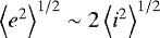$< e^{2} >^{1 / 2} ~ 2 < i^{2} >^{1 / 2}$ $\left< {e}^2 \right>^{1/2}\sim 2 \left< i^2 \right>^{1/2}$ (e.g. Ohtsuki et al. 2002). In this case, the collision timescale increases and M_shep,max would be larger than indicated in Fig. 9. However, it is still unclear whether the energy equipartition works in the resonant trapping where the planetesimal’s eccentricity is excited by the protoplanet. It is clear that both M_shep,max and the planetesimal size distribution depends on the interactions between planetesimals in mean motion resonances. We suggest that this topic should be investigated in detail in future work.

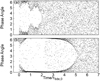Fig. 10

Same as Fig. 7, but (a) for the case with artificial perturbation given by Eq. (50) and (b) without artificial perturbation. Here, we use our reference model with R_pl = 1 × 10⁷cm, τ_tide,0 = 1 × 10⁵ yr and M_p∕M_s = 1 × 10⁻³.

4.1.3 Breakup of resonant trap

High-velocity collisions of planetesimals perturb the orbit of trapped planetesimals and break the resonant trapping. Using numerical simulations, Malhotra (1993b) found that for a planet of 10 M_⊕, resonant trapping is broken with a velocity kick of ≳0.003v_K. Therefore, once M_shep exceeds the threshold value and the trapped planetesimals start to collide with each other, the resonant trapping can be broken by planetesimal collisions. However, the resonant width increases with increasing planetary mass (i.e. breaking the resonant trapping is more difficult for more massive planets; see Eq. (5)) and not all high-velocity collisions lead to the breaking of resonant trapping (see Fig. 6b of Malhotra 1993b). In addition, as mentioned in the previous section, the alignment of the orbits by resonant trapping might reduce the relative velocity of planetesimals. The possibility of resonant breaking by planetesimal collisions need to be investigated in future work. Here we consider the cases where the resonant trapping is broken by planetesimal collisions.

As shown in Sect. 2, planetesimal accretion occurs only in a limited ring-like region within the protoplanetary disk. This accretion process seems different from that found for Earth-mass planets in Tanaka & Ida (1999). In their dynamical simulations Tanaka & Ida (1999) broke the resonant traps instantaneously by exerting artificial perturbations on the trapped planetesimals (see below), supposing that the planetesimals have their motion changed via interactions with other planetesimals. Then, comparing the timescale for the protoplanet’s migration with that for scattering of planetesimals by the migrating protoplanet, they derived a condition required for planetesimal accretion as 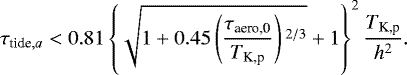$τ_{tide, a} < 0.81 {\sqrt{1 + 0.45 {(\frac{τ_{aero, 0}}{T_{K, p}})}^{2 / 3}} + 1}^{2} \frac{T_{K, p}}{h^{2}} .$ $\begin{align*} \tau_{\textrm{tide},a} < 0.81 \left\{ \sqrt{1+0.45 \left(\frac{\tau_{\textrm{aero,0}}}{T_{\textrm{K,p}}} \right){}^{2/3} } +1 \right\}^2 \frac{T_{\textrm{K,p}}}{h^{2}}.\end{align*}$ (49)

By contrast, when deriving Eq. (32) and also performing the dynamical simulations, we considered an extreme case without modification to the planetesimal’s motion.

Using the artificial perturbation developed in Tanaka & Ida (1997), we perform additional numerical simulations.We randomise the phase angle by adding displacements in orbital elements except a, e, and i. The size of the displacement is set as $Δ θ = 2 π f_{p},$ $\begin{align*} \Delta \theta = 2 \pi f_{\textrm{p}},\end{align*}$ (50)

where f_p is a scaling factor of perturbation strength andrandomly given from − 0.01 to 0.01. We add Δθ to orbital angles (longitude of ascendingnode Ω, longitude of pericentre ϖ and mean longitude at epoch ϵ) every conjunction time. Figure 10 shows the temporal change in the phase angle in the case with (a) and without (b) the artificial perturbations. As shown in panel a, even under strong perturbations (corresponding to up to 1% displacement in the phase angle at every conjunction), mean motion resonances with a Jupiter-mass planet are efficient in trapping planetesimals, and thereby resonance shepherding occurs. This occurs because the resonance width (see Eq. (5)) is larger for Jupiter-mass planets than for Earth-mass planets. The perturbations is, however, found to hasten the breakup of resonant trapping because resonant trapping is weakened and overstable libration is accelerated.

Figure 11 shows the results of the parameter study when varying the planetary mass M_p ∕M_s including the artificial perturbations given by Eq. (50). For comparison, we also show the results without artificial perturbations with open circles in the right panel. Due to the artificial perturbations, the SSP shifts outward (see the left panel) and the total mass of captured planetesimals is reduced (see the right panel). In the left panel the black solid line shows the condition of shepherding obtained in Tanaka & Ida (1999) (see Eq. (49)); planetesimal accretion occurs in regions exterior to it. This black line corresponds to the inner boundary of the SSP for the case where resonant traps are perfectly broken. Although it might seem counter-intuitive, we conclude that without perturbations, resonant trapping shifts the SSP inward and enhances planetesimal accretion due to the effect of accretion bands.

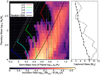Fig. 11

Same as Fig. 5, but for the results of a parameter study for planetary mass M_p with the artificial perturbations (see Eq. (50)). In the right panel the results of a parameter study for planetary mass M_p without the artificial perturbations are plotted as grey circles for comparison.

4.1.4 Ablation of eccentric planetesimals

A highly excited planetesimal has a high relative velocity compared to that of the disk gas. Strong gas drag from the gaseous disk (e.g. Pollack et al. 1986) and generated bow-shock (e.g. Tanaka et al. 2013) heats the planetesimal’s surface and triggers the ablation of volatile materials. Planetesimals trapped in mean motion resonances have eccentric orbits and feel strong gas drag, and therefore ablation is expected to be important. The ablation rate depends on the rate of heat transfer from the ambient disk gas, Λ. We set Λ to range between 0.003 and 0.6 for gas drag heating, and between ~0.01 and ~0.1 for bow shock heating (see Tanaka et al. 2013, and references therein). Recently, Eriksson et al. (2021) explored the possibility of perfect ablation of planetesimals around a massive protoplanet using Λ =C_d∕4, which is the upper limit of the heat transfer rate (D’Angelo & Podolak 2015). According to their nominal model result, ablation of highly excited planetesimals is effective in the inner disk region ≲ 10AU and a large amount of solid material is ablated. The heating process strongly depends on the eccentricity of planetesimals. Using Eqs. (24) and (32), we find that the eccentricity of planetesimals inside the SSP decreases from ~ 0.5 to 0.1. To avoid effective ablation planetesimals must enter the SSP in the outer disk region ≳ 10AU. If the secular resonance triggered by the disk’s gravity is effective, the ablation would be effective in a disk region that is farther out (Nagasawa et al. 2019). On the other hand, if Λ is much smaller than C_d∕4, the ablationof planetesimals would be inefficient.

The investigation presented above concerning planetesimal collision and ablation implies that planetesimal accretion is favoured in the outer disk region ≳10 AU. Detailed future studies that focus on collision and ablation processes are clearly desirable.

4.2 Type II migration with shallow gap

In the classical picture of type II migration (e.g. Lin & Papaloizou 1993), a giant planet migrates with a deep gap opened in the vicinity of its orbit in a gaseous protoplanetary disk. For an extremely deep gap, the radial gas flow toward the central star is stemmed completely by the gap, and consequently the planet migrates with the gaseous disk contracting via viscous diffusion. Recent hydrodynamic simulations, however, reveal that the gap bottom is not so deep and the gas can cross the gap (Kanagawa et al. 2015, 2016, 2017). In this case the planetary migration is not in the classical regime; instead, the torque exerted on the planet similar to that in the type I regime (Kanagawa et al. 2018). Thus, the migration timescale in the new type II regime is written as $τ_{tide, a, II} ~ \frac{1}{2 c} {(\frac{M_{p}}{M_{s}})}^{- 1} {(\frac{r_{p}^{2} Σ_{gap}}{M_{s}})}^{- 1} {(\frac{h_{s}}{r_{p}})}^{2} Ω_{K}^{- 1},$ $\begin{align*}\tau_{\textrm{tide,{a},II}} \sim \frac{1}{2 c} \left(\frac{M_{\textrm{p}}}{M_{\textrm{s}}}\right){}^{-1} \left(\frac{{r_{\textrm{p}}}^2\Sigma_{\textrm{gap}}}{M_{\textrm{s}}}\right){}^{-1} \left(\frac{h_{\textrm{s}}}{r_{\textrm{p}}} \right){}^2 {\Omega_{\textrm{K}}}^{-1}, \end{align*}$ (51)

where c is a constant of the order of unity and Σ_gap is the surface density of disk gas at the gap bottom; Σ_gap depends on the unperturbed surface density of disk gas Σ_gas and is given from the hydrodynamic simulations of Kanagawa et al. (2017) as $Σ_{gap} = \frac{Σ_{gas}}{1 + 0.04 K},$ $\begin{align*}\Sigma_{\textrm{gap}} = \frac{\Sigma_{\textrm{gas}}}{1+0.04 \;\rm K}, \end{align*}$ (52)

with $K = {(\frac{M_{p}}{M_{s}})}^{2} {(\frac{h_{s}}{r_{p}})}^{- 5} α_{vis}^{- 1},$ $\begin{align*} K = \left(\frac{M_{\textrm{p}}}{M_{\textrm{s}}} \right){}^2 \left(\frac{h_{\textrm{s}}}{r_{\textrm{p}}} \right){}^{-5} {\alpha_{\textrm{vis}}}^{-1}, \end{align*}$ (53)

where α_vis is the alpha parameter for disk gas turbulent viscosity (Shakura & Sunyaev 1973). From Eqs. (51) and (52), we obtain $τ_{tide, a, II} ~ \frac{0.02}{c} α_{vis}^{- 1} {(\frac{r_{p}^{2} Σ_{gas}}{M_{p}})}^{- 1} {(\frac{h_{s}}{r_{p}})}^{- 3} Ω_{K}^{- 1},$ $\begin{equation*} \tau_{\textrm{tide},a,\textrm{II}} \sim \frac{0.02}{c} {\alpha_{\textrm{vis}}}^{-1} \left(\frac{{r_{\textrm{p}}}^2\Sigma_{\textrm{gas}}}{M_{\textrm{p}}}\right){}^{-1} \left(\frac{h_{\textrm{s}}}{r_{\textrm{p}}} \right){}^{-3} {\Omega_{\textrm{K}}}^{-1},\end{equation*}$ (54)

for 1 ≪ 0.04 K or $M_{p} ≫ 8 M_{\oplus} {(\frac{α_{vis}}{10^{- 3}})}^{1 / 2} {(\frac{r_{p}}{1 AU})}^{5 (1 - 2 β_{disk}) / 4} .$ $\begin{align*} M_{\textrm{p}} \gg 8 \; M_{\oplus} \left(\frac{\alpha_{\textrm{vis}}}{10^{-3}} \right){}^{1/2} \left(\frac{r_{\textrm{p}}}{1 \;\textrm{AU}} \right){}^{5(1-2\beta_{\textrm{disk}})/4}. \end{align*}$ (55)

Here we discuss the location of SSP and planetesimal accretion onto the protoplanet migrating with Eq. (54).

4.2.1 Location of the accretion sweet spot

The location of the SSP depends on the ratio of the planetary migration to aerodynamic gas drag timescales. The timescale of damping by aerodynamic gas drag τ_aero,0 in the disk mid-plane also depends on the disk structure (see Eq. (16)) as $τ_{aero, 0} = \frac{8 \sqrt{2 π}}{3 C_{d}} {(\frac{Σ_{gas}}{ρ_{pl} R_{pl}})}^{- 1} \frac{h_{s}}{r_{pl}} Ω_{K}^{- 1} .$ $\begin{equation*} \tau_{\textrm{aero,0}} = \frac{8\sqrt{2\pi}}{3 C_{\textrm{d}}} \left(\frac{\Sigma_{\textrm{gas}}}{\rho_{\textrm{pl}} R_{\textrm{pl}}}\right){}^{-1} \frac{h_{\textrm{s}}}{r_{\textrm{pl}}} {\Omega_{\textrm{K}}}^{-1}.\end{equation*}$ (56)

It should be noted that τ_tide,a,II is a functionof r_p, whereas τ_aero,0 is a function of r_pl; $r_{p} / r_{pl} = {((j - 1) / j)}^{2 / 3}$ $r_{\textrm{p}}/r_{\textrm{pl}}=((j-1)/j){}^{2/3}$ for a planetesimal in the j:j − 1 mean motion resonance with the planet. In this case Eq. (56) can be written as a function of r_p as $τ_{aero, 0} = \frac{8 \sqrt{2 π}}{3 C_{d}} {(\frac{Σ_{gas}}{ρ_{pl} R_{pl}})}^{- 1} \frac{h_{s}}{r_{p}} Ω_{K}^{- 1} {(\frac{j - 1}{j})}^{2 γ_{disk} / 3},$ $\begin{equation*} \tau_{\textrm{aero,0}} = \frac{8\sqrt{2\pi}}{3 C_{\textrm{d}}} \left(\frac{\Sigma_{\textrm{gas}}}{\rho_{\textrm{pl}} R_{\textrm{pl}}}\right){}^{-1} \frac{h_{\textrm{s}}}{r_{\textrm{p}}} {\Omega_{\textrm{K}}}^{-1} \left(\frac{j-1}{j}\right){}^{2\gamma_{\textrm{disk}}/3},\end{equation*}$ (57)

with $γ_{disk} = 2 + α_{disk} - β_{disk} .$ $\begin{align*} \gamma_{\textrm{disk}} = 2+\alpha_{\textrm{disk}} -\beta_{\textrm{disk}}.\end{align*}$ (58)

Here, we assume that the planetesimals trapped in mean motion resonances are outside the gap. If the disk viscosity is low, however, the gap slope reaches the locations of the resonances; in that case the damping timescale increases a few times. For simplicity, we neglect this effect.

From Eqs. (54) and (57) the ratio of the two timescales is given by $\frac{τ_{aero, 0}}{τ_{tide, a, II}} = 1 \times 10^{- 6} C^{- 1} {(\frac{M_{p}}{M_{s}})}^{- 1} {(\frac{r_{p}}{1 AU})}^{4 (1 - β_{disk})} {(\frac{j - 1}{j})}^{2 γ_{disk} / 3},$ $\begin{align*} \frac{\tau_{\textrm{aero,0}}}{\tau_{\textrm{tide},a,\textrm{II}}} = 1 \,{\times}\,10^{-6} C^{-1} \left(\frac{M_{\textrm{p}}}{M_{\textrm{s}}}\right){}^{-1} \left(\frac{r_{\textrm{p}}}{1\;\textrm{AU}}\right){}^{4(1-\beta_{\textrm{disk}})} \left(\frac{j-1}{j}\right){}^{2\gamma_{\textrm{disk}}/3},\end{align*}$ (59)

with $C = \frac{2 C_{d}}{c} {(\frac{α_{vis}}{10^{- 3}})}^{- 1} {(\frac{ρ_{pl}}{2 g {cm}^{- 3}})}^{- 1} {(\frac{R_{pl}}{10^{7} cm})}^{- 1} (\frac{M_{s}}{M_{⊙}}) {(\frac{{| h_{s} / r |}_{1 AU}}{0.03})}^{- 4} .$ $\begin{equation*} C = \frac{2C_{\textrm{d}}}{c} \left(\frac{\alpha_{\textrm{vis}}}{10^{-3}}\right){}^{-1} \left(\frac{\rho_{\textrm{pl}}}{2 \,\textrm{g}\,\textrm{cm}^{-3}}\right){}^{-1} \left(\frac{R_{\textrm{pl}}}{10^7~\textrm{cm}}\right){}^{-1} \left(\frac{M_{\textrm{s}}}{M_{\odot}}\right) \left(\frac{\left|h_{\textrm{s}}/r\right|{}_{1\textrm{AU}}}{0.03}\right){}^{-4}\!\!.\end{equation*}$ (60)

Equation (59) indicates that the surface gas density profile only weakly affects the timescale ratio, which does not explicitly depend on Σ_gas and weakly depends on α_disk: ${((j - 1) / j)}^{2 α_{disk} / 3}$ $((j-1)/j){}^{2\alpha_{\textrm{disk}}/3}$ . This means that as the protoplanetary disk evolves, the timescales ratio hardly changes, suggesting that the location of the SSP is fixed.

Assuming α_disk = 1, which is valid in a steady viscous accretion disk except for its outermost region (e.g. Lynden-Bell & Pringle 1974), and β_disk = 1∕4, which is valid in an optically thin disk, and substituting Eq. (59) into Eq. (32), we obtain the semi-major axes of the inner and outer edge of SSP,a_SS,in and a_SS,out, respectively,as $a_{SS, in} = max {\begin{array}{l} 1 C^{1 / 3} {(\frac{M_{p} / M_{s}}{10^{- 3}})}^{2 / 3} {(\frac{j}{j - 1})}^{10 / 9} \\ % 1.41 C^{1 / 3} {(\frac{M_{p} / M_{s}}{10^{- 3}})}^{1 / 3} {\frac{j^{11}}{{(j - 1)}^{5}}}^{1 / 18} \frac{e_{cross}}{0.1} \end{array}} AU,$ $\begin{equation*} a_{\textrm{SS,in}} = \textrm{max} \left. \begin{cases} 1 C^{1/3} \left(\frac{M_{\textrm{p}}/M_{\textrm{s}}}{10^{-3}}\right){}^{2/3} \left(\frac{j}{j-1} \right){}^{10/9} \\%1.4 1 C^{1/3} \left(\frac{M_{\textrm{p}}/M_{\textrm{s}}}{10^{-3}}\right){}^{1/3} \left\{\frac{j^{11}}{(j-1){}^5} \right\}^{1/18} \frac{e_{\textrm{cross}}}{0.1} \end{cases} \right\} \textrm{AU},\end{equation*}$ (61) $a_{SS, out} = 8 C^{1 / 3} {(\frac{M_{p} / M_{s}}{10^{- 3}})}^{1 / 3} {\frac{j^{11}}{{(j - 1)}^{14}}}^{1 / 18} AU .$ $\begin{equation*} a_{\textrm{SS,out}} = 8 C^{1/3} \left(\frac{M_{\textrm{p}}/M_{\textrm{s}}}{10^{-3}}\right){}^{1/3} \left\{ \frac{j^{11}}{(j-1){}^{14}} \right\}^{1/18} \textrm{AU}.\end{equation*}$ (62)

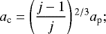
Figure 12 shows exoplanets identified so far and the predicted location of the SSP in the a_p –M_p plane for C = 10. The SSP locates from ~ 1 AU to ~ 30 AU and shifts outward with increasing planetary mass. The red and black symbols show exoplanets observed using the transit method and the radial-velocity method, respectively (http://exoplanet.eu). Given that planetary growth occurs via runaway gas accretion, followed by inward migration, the evolution path of a gas giant planet can be drawn from the bottom right to the top left in the a_p –M_p plane (e.g. Ida & Lin 2004; Mordasini et al. 2009). If runaway gas accretion begins in the outer disk region, which might be favoured for planetary core formation because of the increasing isolation mass of protoplanet (e.g. Armitage 2010), the exoplanets currently observed in the region interior to the SSP must have crossed the SSP during their formation stages.

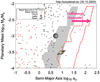Fig. 12

Distribution of confirmed exoplanets in the semi-major axis vs. planetary mass plane (http://exoplanet.eu). The black points are exoplanets observed by the radial-velocity method. The red points are exoplanets observed by the radial-velocity + transit methods. As for masses of exoplanets indicated with the black points, the observed values of M_p sin i are used. The grey area shows the theoretical sweet spot for planetesimal capture given by Eqs. (61) and (62) with C = 10. The red dashed line shows the theoretical sweet spot for planetesimal capture with C = 10³, which corresponds to the case where collisional cascade have broken planetesimals down to R_pl ≲ 10⁵ cm.

4.2.2 Maximum mass of planetesimals shepherded into the SSP

The total mass of accreted planetesimals depends on the number of planetesimals that are shepherded into the SSP. By substituting Eqs. (4), (54), and (62) into Eq. (45), we can estimate M_shep,max when the protoplanet reaches the outer edge of the SSP. In this case, M_shep,max weakly depends on α_vis, ρ_pl, R_pl, and $M_{p}^{- 1}$ ${M_{\textrm{p}}}^{-1}$ (− 1∕4 powers of each value), but linearly depends on $\tan $ $\tan \left$ , Σ_gas,0 and $T_{0}^{- 1}$ ${T_{\textrm{0}}}^{-1}$ . Here we adopt the optically thick disk of T₀ = 140 K (Sasselov & Lecar 2000) and consider two disks with Σ_gas,0 = 1400 g cm⁻² and 800 g cm⁻². The former disk corresponds to the massive disk of total mass 0.1 M_s and typical radius 100 AU. Figure 13 shows M_shep,max as a function of planetary mass M_p∕M_s. We find that a few tens of M_⊕ of planetesimals can be shepherded into the SSP before initiating collisional cascade even with $\tan = 10^{- 3}$ $\tan\left=10^{-3}$ . For the capture of several tens or more planetesimals, the effect enhancing $\tan $ $\tan\left$ needs to be considered.

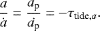
It is important to note that M_shep,max only provides the maximum mass of planetesimals shepherded into the SSP and not the mass of planetesimals that can be captured by the protoplanet. The numerical simulations we presented in Sect. 3 suggest that ~ 30% of the shepherded planetesimals are captured by the protoplanet. This accretion efficiency, however, depends on various parameters such as the inclination of planetesimals (Tanaka & Ida 1999) and the planetary capture radius (Inaba & Ikoma 2003). In addition, the initial semi-major axis of planetesimals also affects the capture efficiency because of the mean motion resonances. A detailed investigation of the accretion efficiency under various conditions should be conducted in future research.

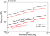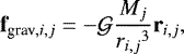
Fig. 13

Maximum mass of planetesimals shepherded into the SSP without active planetesimal collisions M_max,shep as a functionof planetary mass M_p. Here, thecase is considered where the protoplanet migrates with the type II regime obtained by Kanagawa et al. (2018) (see Eq. (51)). The solid and dashed lines show the cases of = 10⁻³ and 10⁻², respectively. The black and red lines are cases of massive disk with Σ_gas,0 = 1400 g cm⁻² and 800 g cm⁻², respectively. The parameters used in this plot are the optically thick disk of T₀ = 140 K, the disk viscosity α_vis = 10⁻³, the size of planetesimal R_pl = 10⁷ cm, and the planetesimal density ρ_pl = 1 g cm⁻³. The scaling parameter of the location of the SSP C is obtained as C = 17.

4.3 Heavy-element enrichment of giant planets

If giant planets cross the sweet spot during the migration phase, planetesimal accretion could take place. If several tens Earth-masses of planetesimals were shepherded into the SSP as shown in Fig. 13, we would expect a clear difference in the total heavy-element mass of planets depending on whether they migrated interior or exterior to the SSP. If this difference between planetary populations is observed, it could confirm that planetesimal accretion is a significant process that takes place during planetary migration. However, once the collisional cascade occurs, the location of the SSP moves to the outer disk region and the metallicity difference between the populations would be reduced. It is therefore still unclear whether such a difference is detectable.

Currently, there are no estimated metallicities for giant exoplanets within the outer disk region (i.e. at distances ≳ 10 AU). To estimate the metallicity of giant exoplanets, measurements of the radius, mass, and age of the planet are required. At the moment, data of the masses and radii of cold giant planets are still unavailable. Nevertheless, the upcoming decades are expected to provide vast observations thanks to various missions. Wide field observations, such as TESS (Transiting Exoplanet Survey Satellite, Ricker et al. 2014) and Plato (Rauer et al. 2014), will increase the number of cold giant planets. Follow-up observations using precise radial-velocity measurement, such as HARPS (High-Accuracy Radial velocity PlanetSearcher, Mayor et al. 2003) and ESPRESSO (Echelle Spectrograph for Rocky Exo-planet and Stable Spectroscopic Observation, Pepe et al. 2010), and precise transit measurement, such as NGTS (Wheatley et al. 2018) and WASP (Wide Angle Search for Planets, Pollacco et al. 2006), are suitable for obtaining the masses and radii of giant planets at large radial distances. In addition, the high-dispersion coronagraphy technique (e.g. Kotani et al. 2020) could constrain the atmospheric composition of cold giant planets. Next generation observations will constrain the main source of heavy elements.

In this study, we focus on planetesimal accretion and consider it as the main source of heavy-element enrichment in gas giant planets. However, other various processes could also lead to heavy-element enrichment. The metallicity of the gaseous disk can be enriched by the sublimation of dust grains and pebbles crossing each ice lines (Booth et al. 2017; Booth & Ilee 2019). The accretion of these enriched disk gas brings massive heavy elements into gas giant planets (Schneider & Bitsch 2021). Giant impacts have also been investigated as a source of enrichment (Ikoma et al. 2006; Liu et al. 2015, 2019; Ginzburg & Chiang 2020; Ogihara et al. 2021). By combining the effects of pebble accretion and giant impacts, Ogihara et al. (2021) found that up to ~ 100 M_⊕ of heavy elements can be accreted by a giant planet through multi-giant impacts of Neptune-mass planets.

In order to determine what is the main source of the heavy-element enrichment in giant exoplanets, other observational information such as elemental ratios (e.g. refractory-to-volatile, C/O, O/H) is valuable. In recent observations, the existence of TiO and VO in hot Jupiters is suggested by the transmission spectrum analysis (Evans et al. 2016; Chen et al. 2021). The amount of these refractory materials is useful for constraining the dominant process of heavy-element accretion. The accretion of massive refractory materials is only possible through solid accretion; thus, using the information of refractory materials, we can constrain whether the heavy elements are brought by solid accretion or gas accretion.

The elemental ratio of volatile materials also provides information on the accretion process of heavy elements (e.g. Madhusudhan et al. 2014; Notsu et al. 2020; Turrini et al. 2021; Schneider & Bitsch 2021). Turrini et al. (2021) investigated the effect of planetesimal accretion on elemental ratios of volatile materials such as C/O, N/O, or S/N. They considered a Jupiter-mass planet in a typical disk model; however, the relative position between the SSP and each ice lines changes with the planetary mass and disk conditions. The elemental ratio of planetesimals shepherded into the SSP would depend on the evolution pathways of the giant planets on the a_p –M_p plane and disk conditions. We hope to further investigate the link between elemental ratios and the formation history in follow-up studies. This is highly relevant since future missions like JWST and Ariel will provide accurate measurements of the atmospheric composition of gaseous planets that can then be used to better understand the planetary origin.

5 Summary and conclusions

Planetesimal accretion during planetary migration could lead to a significant enrichment of giant planets with heavy elements. As revealed in Shibata et al. (2020), planetesimal accretion occurs in a sweet spot for planetesimal accretion (SSP), where planetesimals can be efficiently captured by the migrating planet. By performing dynamical simulations for planetesimals with a migrating planet, Shibata et al. (2020) demonstrated that the SSP emerges due to shepherding processes caused by aerodynamic gas drag and mean motion resonances. However, they conducted no detailed analysis of the nature (especially, the location) of the SSP, and therefore in this paper we focused on the nature of the accretion sweet spot.

In Sect. 2, we analytically derived an equation describing the location of the SSP and found the following that the SSP is regulated by the ratio of the damping timescale for the planetesimal eccentricity due to aerodynamic gas drag to the migration timescale of the planet, and that the SSP also depends on the planetary mass because the accretion bands change with the relative positions between the mean motion resonances and the feeding zone.

In Sect. 3, we performed numerical simulations and confirmed that the derived conditions reproduce the numerical results well. In Sect. 4, we discussed the effect of planetesimal collisions and ablation during the shepherding process. These effects would be important for inner disk regions ≲ 10 AU and put other constraint for planetesimal accretion process. If the migration timescale is inversely proportional to the disk gas surface density (e.g. Kanagawa et al. 2018), the timescales ratio is rather insensitive to the structure of the protoplanetary disk. Therefore, the location of the SSP is fixed during the evolution of the protoplanetary disk.

Finally, we discussed the effect of the SSP on the heavy-element enrichment of gas giant planets. We suggest that the existence of the SSP makes a difference in the heavy-element mass between planets observed in the regions interior and exterior to the SSP. The detailed chemical composition of gas giant planets, such as the refractory-to-volatile ratio or C/O ratio, would be also affected by the location of the SSP. If such compositional features can be observed, it could be a piece of the evidence of planetesimal accretion during planetary migration. Future observations in the upcoming decades will reveal whether planetesimal accretion is a main source of heavy elements in giant planets, and therefore advance our understanding of their origin.

Acknowledgements

S.S. and R.H. acknowledge support from the Swiss National Science Foundation (SNSF) under grant 200020_188460. Part of this work was supported by the German Deutsche Forschungsgemeinschaft, DFG project number Ts 17/2–1 and by JSPS Core-to-Core Program “International Network of Planetary Sciences (Planet²)” and JSPS KAKENHI Grant Numbers 17H01153 and 18H05439.

Appendix A Model descriptions

A.1 Equations of motion

The equation of motion is given by $\frac{d r_{i}}{d t} = \sum_{i \neq j} f_{grav, i, j} + f_{aero} + f_{tide},$ $\begin{align*} \frac{\textrm{d} \textbf{r}_i }{\textrm{d} t} = \sum_{i\neq j} \textbf{f}_{\textrm{grav},i,j} + \textbf{f}_{\textrm{aero}} +\textbf{f}_{\textrm{tide}},\end{align*}$ (A.1)

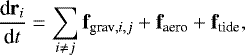
where r_i is the position vector relative to the initial (i.e. t = 0) mass centre of the star-planet-planetesimals system; f_grav,i,j is the mutual gravity between particles i and j given by $f_{grav, i, j} = - G \frac{M_{j}}{r_{i, j}^{3}} r_{i, j},$ $\begin{align*} \textbf{f}_{\textrm{grav},i,j} = - \mathcal{G} \frac{M_j}{{r_{i,j}}^3} \textbf{r}_{i,j},\end{align*}$ (A.2)

with r_i,j being the position vector of particle i relative to particle j (r_i,j ≡|r_i,j|); M_j is the mass of particle j; $G$ $\mathcal{G}$ is the gravitational constant; f_aero is the aerodynamic gas drag; and f_tide is the gravitational tidal drag from the protoplanetary disk gas. The central star, planet, and planetesimals are denoted by the subscripts i (or j) = 1, 2, and ≥ 3, respectively. The planetesimals are treated as test particles; therefore, f_grav,i,j = 0 in Eq. (A.1) for j ≥ 3. The aerodynamic gas drag force and the tidal drag force are given respectively by $f_{aero} = - \frac{u}{τ_{aero}},$ $\begin{equation*} \textbf{f}_{\textrm{aero}} = -\frac{\textbf{u}}{\tau_{\textrm{aero}}},\end{equation*}$ (A.3) $f_{tide} = - \frac{v_{p}}{2 τ_{tide, a}},$ $\begin{equation*} \textbf{f}_{\textrm{tide}} = - \frac{\textbf{v}_{\textrm{p}}}{2 \tau_{\textrm{tide},a}}, \end{equation*}$ (A.4)

with $τ_{aero} = \frac{2 m_{pl}}{C_{d} π R_{pl}^{2} ρ_{gas} u} = τ_{aero, 0} \frac{v_{K}}{u} .$ $\begin{align*} \tau_{\textrm{aero}} = \frac{2 m_{\textrm{pl}}}{ C_{\textrm{d}} \pi R_{\textrm{pl}}^2 \rho_{\textrm{gas}} u} = \tau_{\textrm{aero, 0}} \frac{v_{\textrm{K}}}{u}.\end{align*}$ (A.5)

Here u = v_pl −v_gas (u = |u|) is the planetesimal’s velocity (v_pl) relative to the ambient gas (v_gas), Given the range of the planetesimal mass (~ 10¹⁶–10²²g) and planet (~ 10³⁰g), we assume f_tide = 0 for the former and f_aero = 0 for the latter. The central star is not affected by f_aero and f_tide.

A.2 Gas disk

The protoplanetary disk is assumed to be vertically isothermal, and the gas density ρ_gas is expressed as $ρ_{gas} = \frac{Σ_{gas}}{\sqrt{2 π} h_{s}} \exp (- \frac{z^{2}}{2 h_{s}^{2}}),$ $\begin{align*}\rho_{\textrm{gas}} = \frac{\Sigma_{\textrm{gas}}}{\sqrt{2 \pi} h_{\textrm{s}}} \exp \left(-\frac{z^2}{2 {h_{\textrm{s}}}^2} \right), \end{align*}$ (A.6)

where z is the height from the disk mid-plane and h_s is the disk’s scale height. The aspect ratio of the protoplanetary disk is given by $\frac{h_{s}}{r} = \frac{c_{s}}{r Ω_{K}},$ $\begin{align*} \frac{h_{\textrm{s}}}{r} = \frac{c_{\textrm{s}}}{r\Omega_{\textrm{K}}}, \end{align*}$ (A.7)

where Ω_K is the Kepler angular velocity and c_s is the isothermal sound speed of the disk gas. The sound speed is given as $c_{s} = \sqrt{\frac{k_{B} T_{disk}}{μ_{disk} m_{H}}} \propto r^{- β disk},$ $\begin{align*} c_{\textrm{s}} = \sqrt{\frac{k_{\textrm{B}} T_{\textrm{disk}}}{\mu_{\textrm{disk}} m_{\textrm{H}}}} \propto r^{-\beta{\textrm{disk}}}, \end{align*}$ (A.8)

where k_B is the Boltzmann constant and μ_disk is the mean molecular weight in units of proton mass, m_H. In this study μ_disk is set as 2.3 and the aspect ratio of the disk gas at 1AU is ~ 0.03.

The gasin the protoplanetary disk rotates at sub-Keplerian velocity because of pressure gradient, namely v_gas = (1 − η_gas)rΩ_K, where η_gas is ≪ 1 and is given as $η_{gas} \equiv - \frac{1}{2} {(\frac{h_{s}}{r})}^{2} \frac{d \ln P_{gas}}{d \ln r},$ $\begin{equation*} \eta_{\textrm{gas}} \equiv \mathbf{-} \frac{1}{2} \left(\frac{h_{\textrm{s}}}{r} \right){}^2 \frac{\textrm{d} \ln P_{\textrm{gas}}}{\textrm{d} \ln r},\end{equation*}$ (A.9) $= \frac{1}{2} {(\frac{h_{s}}{r})}^{2} [\frac{3}{2} (1 - \frac{z^{2}}{h_{s}^{2}}) + α_{disk} + β_{disk} (1 + \frac{z^{2}}{h_{s}^{2}})],$ $\begin{equation*} = \frac{1}{2} \left(\frac{h_{\textrm{s}}}{r} \right){}^2 \left[ \frac{3}{2} \left(1 - \frac{z^2}{{h_{\textrm{s}}}^2} \right) +\alpha_{\textrm{disk}} +\beta_{\textrm{disk}} \left(1+\frac{z^2}{{h_{\textrm{s}}}^2} \right) \right], \end{equation*}$ (A.10)

where P_gas is the gas pressure.

A.2 Planetesimals

The surface number density of planetesimals is given as Σ_solid∕m_pl, which gives a maximum value of ~ 10⁶ ∕AU². To speed up the numerical integration, we follow the orbital motion of super-particles. The surface number density of super-particles n_s is given as $n_{s} = n_{s, 0} {(\frac{r}{1 AU})}^{- α_{sp}},$ $\begin{align*} n_{\textrm{s}} = n_{\textrm{s,0}} \left(\frac{r}{1 \textrm{AU}} \right){}^{-\alpha_{\textrm{sp}}}, \end{align*}$ (A.11)

where $n_{s, 0} = \frac{N_{sp}}{2 π} \frac{2 - α_{sp}}{{(a_{pl, out} / 1 AU)}^{2 - α_{sp}} - {(a_{pl, in} / 1 AU)}^{2 - α_{sp}}} [\frac{1}{{AU}^{2}}];$ $\begin{align*} n_{\textrm{s,0}} = \frac{N_{\textrm{sp}}}{2 \pi} \frac{2 -\alpha_{\textrm{sp}}} {\left(a_{\textrm{pl,out}}/1\textrm{AU}\right){}^{2-\alpha_{\textrm{sp}}} -\left(a_{\textrm{pl,in}}/1\textrm{AU}\right){}^{2-\alpha_{\textrm{sp}}} } \left[\frac{1}{\textrm{AU}^2}\right]; \end{align*}$ (A.12)

here N_sp is the total number of super-particles used in a given simulation. In our simulation we set N_sp = 12, 000 and α_sp = 1 to distribute super-particles uniformly in the radial direction. The mass per super-particle M_sp is given by $M_{sp} (a_{0}) = \frac{Σ_{solid} (a_{0})}{n_{s} (a_{0})},$ $\begin{align*} M_{\textrm{sp}} (a_{\textrm{0}}) = \frac{\Sigma_{\textrm{solid}} (a_{\textrm{0}})}{n_{\textrm{s}} (a_{\textrm{0}})}, \end{align*}$ (A.13)

where a₀ is the initial semi-major axis of the super-particle.

Although planetesimals are treated as test particles in our simulations, assuming that planetesimals are in reality scattered by their mutual gravitational interaction, for eccentricity and inclination we adopt the Rayleigh distribution as the initial eccentricities e and inclinations i of planetesimals. We set $< e^{2} >^{1 / 2} = 2 < i^{2} >^{1 / 2} = 10^{- 3}$ $\left< e^2 \right>^{1/2}=2\left< i^2 \right>^{1/2}=10^{-3}$ . The orbital angles Ω, ϖ, and ϵ are distributed uniformly.

During the orbital integration, we judge that a super-particle has been captured by the planet once (i) the super-particle enters the planet’s envelope or (ii) its Jacobi energy becomes negative in the Hill sphere. The planet’s radius R_p is calculated as $R_{p} = {(\frac{3 M_{p}}{4 π ρ_{p}})}^{1 / 3},$ $\begin{align*}R_{\textrm{p}} = \left(\frac{3 M_{\textrm{p}}}{4 \pi \rho_{\textrm{p}}} \right){}^{1/3}, \end{align*}$ (A.14)

where ρ_p is the planet’s mean density. The planet’s radius is assumed to be extended shortly after formation and the density is set to ρ_p = 0.125 g cm⁻³, corresponding to a planet radius twice as large as Jupiter’s current radius.

References

Aarseth, S. J. 1985, in IAU Symposium, 113, Dynamics of Star Clusters, eds. J. Goodman, & P. Hut, 251 [CrossRef] [Google Scholar]
Adachi, I., Hayashi, C., & Nakazawa, K. 1976, Progr. Theor. Phys., 56, 1756 [Google Scholar]
Alibert, Y., Mordasini, C., Benz, W., & Winisdoerffer, C. 2005, A&A, 434, 343 [NASA ADS] [CrossRef] [EDP Sciences] [Google Scholar]
Armitage, P. J. 2010, Astrophysics of Planet Formation (Cambridge, UK: Cambridge University Press) [Google Scholar]
Batygin, K. 2015, MNRAS, 451, 2589 [NASA ADS] [CrossRef] [Google Scholar]
Batygin, K., & Laughlin, G. 2015, Proc. Natl. Acad. Sci. USA, 112, 4214 [CrossRef] [Google Scholar]
Benz, W., & Erik, A. 1999, Icarus, 142, 5 [NASA ADS] [CrossRef] [Google Scholar]
Booth, R. A., & Ilee, J. D. 2019, MNRAS, 487, 3998 [CrossRef] [Google Scholar]
Booth, R. A., Clarke, C. J., Madhusudhan, N., & Ilee, J. D. 2017, MNRAS, 469, 3994 [Google Scholar]
Chen, G., Pallé, E., Parviainen, H., Murgas, F., & Yan, F. 2021, ApJ, 913, L16 [NASA ADS] [CrossRef] [Google Scholar]
D’Angelo, G., & Podolak, M. 2015, ApJ, 806, 203 [Google Scholar]
Debras, F., & Chabrier, G. 2019, ApJ, 872, 100 [Google Scholar]
Dermott, S. F., Malhotra, R., & Murray, C. D. 1988, icarus, 76, 295 [NASA ADS] [CrossRef] [Google Scholar]
Dohnanyi, J. S. 1969, J. Geophys. Res., 74, 2531 [Google Scholar]
Eriksson, L. E. J., Ronnet, T., & Johansen, A. 2021, A&A, 648, A112 [NASA ADS] [CrossRef] [EDP Sciences] [Google Scholar]
Evans, T. M., Sing, D. K., Wakeford, H. R., et al. 2016, ApJ, 822, L4 [NASA ADS] [CrossRef] [Google Scholar]
Fabrycky, D. C., Lissauer, J. J., Ragozzine, D., et al. 2014, ApJ, 790, 146 [Google Scholar]
Ginzburg, S., & Chiang, E. 2020, MNRAS, 498, 680 [NASA ADS] [CrossRef] [Google Scholar]
Goldreich, P. 1965, MNRAS, 130, 159 [NASA ADS] [Google Scholar]
Goldreich, P., & Schlichting, H. E. 2014, ApJ, 147, 32 [CrossRef] [Google Scholar]
Guillot, T. 1999, Planet. Space Sci., 47, 1183 [NASA ADS] [CrossRef] [Google Scholar]
Guillot, T., Santos, N. C., Pont, F., et al. 2006, A&A, 453, L21 [CrossRef] [EDP Sciences] [Google Scholar]
Guo, K., & Kokubo, E. 2021, AJ, 162, 115 [NASA ADS] [CrossRef] [Google Scholar]
Hayashi, C. 1981, Progr. Theor. Phys. Suppl., 70, 35 [Google Scholar]
Hayashi, C., Nakazawa, K., & Adachi, I. 1977, Publ. Astron. Soc. Jpn., 29, 163 [Google Scholar]
Helled, R., & Guillot, T. 2013, ApJ, 767, 113 [CrossRef] [Google Scholar]
Helled, R., Werner, S., Dorn, C., et al. 2021, Exp. Astron., in press [arXiv:2103.08481] [Google Scholar]
Ida, S., & Lin,D. N. C. 2004, ApJ, 604, 388 [Google Scholar]
Ida, S., & Nakazawa, K. 1989, A&A, 220, 293 [NASA ADS] [Google Scholar]
Ida, S., Tanaka, H., Johansen, A., Kanagawa, K. D., & Tanigawa, T. 2018, ApJ, 864, 77 [NASA ADS] [CrossRef] [Google Scholar]
Ikoma, M., Guillot, T., Genda, H., Tanigawa, T., & Ida, S. 2006, ApJ, 650, 1150 [NASA ADS] [CrossRef] [Google Scholar]
Inaba, S., & Ikoma, M. 2003, A&A, 410, 711 [NASA ADS] [CrossRef] [EDP Sciences] [Google Scholar]
Kanagawa, K. D., Tanaka, H., Muto, T., Tanigawa, T., & Takeuchi, T. 2015, MNRAS, 448, 994 [NASA ADS] [CrossRef] [Google Scholar]
Kanagawa, K. D., Muto, T., Tanaka, H., et al. 2016, Publ. Astron. Soc. Jpn., 68, 43 [CrossRef] [Google Scholar]
Kanagawa, K. D., Tanaka, H., Muto, T., & Tanigawa, T. 2017, Publ. Astron. Soc. Jpn., 69 [Google Scholar]
Kanagawa, K. D., Tanaka, H., & Szuszkiewicz, E. 2018, ApJ, 861, 140 [Google Scholar]
Kotani, T., Kawahara, H., Ishizuka, M., et al. 2020, in SPIE Conf. Ser., 11448, 1144878 [NASA ADS] [Google Scholar]
Leinhardt, Z. M., & Stewart, S. T. 2009, Icarus, 199, 542 [NASA ADS] [CrossRef] [Google Scholar]
Lin, D. N. C., & Papaloizou, J. C. B. 1993, in Protostars and Planets III, eds. E. H. Levy, & J. I. Lunine, 749 [Google Scholar]
Liu, S. F., Agnor, C. B., Lin, D. N., & Li, S. L. 2015, MNRAS, 446, 1685 [NASA ADS] [CrossRef] [Google Scholar]
Liu, S.-F., Hori, Y., Müller, S., et al. 2019, Nature, 572, 355 [NASA ADS] [CrossRef] [Google Scholar]
Lynden-Bell, D., & Pringle, J. E. 1974, MNRAS, 168, 603 [Google Scholar]
Madhusudhan, N., Amin, M. A., & Kennedy, G. M. 2014, ApJ, 794, 12 [Google Scholar]
Makino, J., & Aarseth, S. J. 1992, Publ. Astron. Soc. Jpn., 44, 141 [Google Scholar]
Malhotra, R. 1993a, Icarus, 106, 264 [NASA ADS] [CrossRef] [Google Scholar]
Malhotra, R. 1993b, Nature, 365, 819 [CrossRef] [Google Scholar]
Mankovich, C., & Fuller, J. 2021, Nat. Astron., 5, 1103 [NASA ADS] [CrossRef] [Google Scholar]
Mayor, M., Pepe, F., Queloz, D., et al. 2003, The Messenger, 114, 20 [NASA ADS] [Google Scholar]
Miller, N., & Fortney, J. J. 2011, ApJ, 736, L29 [NASA ADS] [CrossRef] [Google Scholar]
Mordasini, C. 2018, in Handbook of Exoplanets, 2425 [CrossRef] [Google Scholar]
Mordasini, C., Alibert, Y., & Benz, W. 2009, A&A, 501, 1139 [CrossRef] [EDP Sciences] [Google Scholar]
Movshovitz, N., Fortney, J. J., Mankovich, C., Thorngren, D., & Helled, R. 2020, ApJ, 891, 109 [Google Scholar]
Murray, C. D., & Dermott, S. F. 1999, Solar System Dynamics (Cambridge, UK: Cambridge University Press) [Google Scholar]
Nagasawa, M., Tanaka, K. K., Tanaka, H., et al. 2019, ApJ, 871, 110 [NASA ADS] [CrossRef] [Google Scholar]
Notsu, S., Eistrup, C., Walsh, C., & Nomura, H. 2020, MNRAS, 499, 2229 [Google Scholar]
Ogihara, M., Hori, Y., Kunitomo, M., & Kurosaki, K. 2021, A&A, 648, L1 [NASA ADS] [CrossRef] [EDP Sciences] [Google Scholar]
Ohtsuki, K., Stewart, G. R., & Ida, S. 2002, Icarus, 155, 436 [Google Scholar]
Pepe, F. A., Cristiani, S., Rebolo Lopez, R., et al. 2010, SPIE Conf. Ser., 7735, 77350F [Google Scholar]
Podolak, M., Haghighipour, N., Bodenheimer, P., Helled, R., & Podolak, E. 2020, ApJ, 899, 45 [NASA ADS] [CrossRef] [Google Scholar]
Pollacco, D., Skillen, I., Cameron, A., et al. 2006, PASP, 118, 1407 [NASA ADS] [CrossRef] [Google Scholar]
Pollack, J. B., Podolak, M., Bodenheimer, P., & Christofferson, B. 1986, Icarus, 67, 409 [Google Scholar]
Rauer, H., Catala, C., Aerts, C., et al. 2014, Exp. Astron., 38, 249 [Google Scholar]
Ricker, G. R., Winn, J. N., Vanderspek, R., et al. 2014, SPIE Conf. Ser., 9143, 914320 [Google Scholar]
Sasselov, D. D., & Lecar, M. 2000, ApJ, 528, 995 [Google Scholar]
Saumon, D., & Guillot, T. 2004, ApJ, 609, 1170 [NASA ADS] [CrossRef] [Google Scholar]
Schneider, A. D., & Bitsch, B. 2021, How drifting and evaporating pebbles shape giant planets I: Heavy element content and atmospheric C/O, Tech. rep. [Google Scholar]
Shakura, N. I., & Sunyaev, R. A. 1973, A&A, 24, 337 [NASA ADS] [Google Scholar]
Shibata, S., & Ikoma, M. 2019, MNRAS, 487, 4510 [NASA ADS] [CrossRef] [Google Scholar]
Shibata, S., Helled, R., & Ikoma, M. 2020, A&A, 633, 13 [Google Scholar]
Shiraishi, M., & Ida, S. 2008, ApJ, 684, 1416 [NASA ADS] [CrossRef] [Google Scholar]
Tanaka, H., & Ida, S. 1997, Icarus, 125, 302 [NASA ADS] [CrossRef] [Google Scholar]
Tanaka, H., & Ida, S. 1999, Icarus, 139, 350 [NASA ADS] [CrossRef] [Google Scholar]
Tanaka, K. K., Yamamoto, T., Tanaka, H., et al. 2013, ApJ, 764, 120 [NASA ADS] [CrossRef] [Google Scholar]
Thorngren, D. P., Fortney, J. J., Murray-Clay, R. A., & Lopez, E. D. 2016, ApJ, 831, 64 [NASA ADS] [CrossRef] [Google Scholar]
Turrini, D., Schisano, E., Fonte, S., et al. 2021, ApJ, 909, 40 [Google Scholar]
Wahl, S. M., Hubbard, W. B., Militzer, B., et al. 2017, Geophys. Res. Lett., 44, 4649 [CrossRef] [Google Scholar]
Wheatley, P. J., West, R. G., Goad, M. R., et al. 2018, MNRAS, 475, 4476 [Google Scholar]
Yu, Q., & Tremaine, S. 2001, AJ, 121, 1736 [NASA ADS] [CrossRef] [Google Scholar]
Zhou, J., & Lin, D. N. C. 2007, ApJ, 666, 447 [NASA ADS] [CrossRef] [Google Scholar]

All Tables

Table 1

Values of the secular term f_s and the directterm f_d for the first-order mean motion resonances.

In the text

Table 2

Parameters used in the reference model.

In the text

All Figures

Fig. 1

Orbital evolution of a planetesimal initially located at 13.8 AU dictated via the gravitational interaction with a migrating Jupiter-mass protoplanet. The dots and crosses show the locations of the planetesimal and the protoplanet, respectively, and are colour-coded according to time. In this simulation the surface density of disk gas is set to that of the minimum-mass solar nebula and aerodynamic gas drag is included. Here, the protoplanet migrates from 15.0 AU with a migration rate of 10⁵ AU yr⁻¹. For the details of the numerical simulation, see Sect. 3.

In the text

Fig. 2

Ratio of the crossing timescale τ_cross (Eq. (3)) to the libration timescale τ_lib (Eq. (9)) as a function of the planetesimal’s semi-major axis. Here, the type II regime obtained in Kanagawa et al. (2018) is considered for the migration timescale τ_tide,a. The solid, dash-dotted, and dotted lines show the cases of the planet-to-star mass ratio M_p ∕M_s= 10⁻², 10⁻³, and 10⁻⁴, respectively. Shown are the inner first-order mean motion resonances (or j:j − 1 resonances): thick lines are for j = 2 and thin lines are for j = 3. To calculate the migration timescale, the same disk model was used as in Ida et al. (2018). The disk accretion rate, disk viscosity parameter, and disk aspect ratio is set to 10⁻⁸ M_⊙ yr⁻¹, 10⁻³, and 0.03r^1∕4, respectively.

In the text

	Fig. 3 Dependence of the crossing point eccentricity e_cross (see Eq. (27)) on the planet-to-star mass ratio M_p∕M_s for four different cases: j = 2 (solid), j = 3 (dashed), j = 4 (dash-dotted), and j = 5 (dotted).
In the text

	Fig. 4 Planetesimal accretion rate vs. the semi-major axis of the migrating planet. The vertical solid lines showthe boundaries of the SSP given by Eq. (32). The red lines are for the case of j = 2 and the green lines are for j = 3. The filled areas show the SSP.
In the text

Fig. 5

Results of the parameter study regarding the size of planetesimals R_pl. Left: planetesimal accretion rate shown as a colour contour on a plane of the semi-major axis of the migrating protoplanets and the radius of the planetesimals, The analytically predicted inner and outer boundaries of the sweet spot are indicated with solid and dashed lines, respectively. The red lines are for j = 2 and the green lines are for j = 3. Right: total mass of captured planetesimals as a function of the planetesimal radius.

In the text

	Fig. 6 Same as Fig. 5, but for the results of the parameter study regarding the migration timescale τ_tide,0. The grey circles in the right panel show the results of the parameter study regarding the size of planetesimals, R_pl, for comparison using the fraction of timescales τ_aero,0∕τ_tide,a on the vertical axis.
In the text

Fig. 7

Change in the phase angle of a planetesimal initially located at a₀ = 13.8 AU. Panel a shows the case of τ_tide,0 = 1 × 10⁴ yr and panel b shows the case of τ_tide,0 = 1 × 10⁵ yr. In panel a, the phase angle oscillates indicating that the resonant trapping is unstable due to fast planetary migration. Then, the resonant trapping is broken earlier in the case of panel a than that shown in panel b.

In the text

Fig. 8

Same as Fig. 5, but for the results of the parameter study when varying the protoplanet’s mass, M_p. The red, green, sky blue, and blue lines represent the SSP inner (solid lines) and outer (dashed lines) boundaries determined by the resonant trapping, which is predicted by Eq. (32) for j = 2, 3, 4, and 5, respectively. The coloured lines change into the grey lines once the protoplanet mass exceeds a threshold value, beyond which the accretion bands disappear (see Fig. 3).

In the text

	Fig. 9 Maximum mass of planetesimals that can be shepherded in mean motion resonances without effective mutual collisions. We show the cases of R_pl = 10⁷ cm and <i> = 10⁻³. The solid, dashed, and dotted lines correspond to τ_tide,a = 10⁶ yr, 10⁵ yr, and 10⁴ yr, respectively.
In the text

	Fig. 10 Same as Fig. 7, but (a) for the case with artificial perturbation given by Eq. (50) and (b) without artificial perturbation. Here, we use our reference model with R_pl = 1 × 10⁷cm, τ_tide,0 = 1 × 10⁵ yr and M_p∕M_s = 1 × 10⁻³.
In the text

	Fig. 11 Same as Fig. 5, but for the results of a parameter study for planetary mass M_p with the artificial perturbations (see Eq. (50)). In the right panel the results of a parameter study for planetary mass M_p without the artificial perturbations are plotted as grey circles for comparison.
In the text

Fig. 12

Distribution of confirmed exoplanets in the semi-major axis vs. planetary mass plane (http://exoplanet.eu). The black points are exoplanets observed by the radial-velocity method. The red points are exoplanets observed by the radial-velocity + transit methods. As for masses of exoplanets indicated with the black points, the observed values of M_p sin i are used. The grey area shows the theoretical sweet spot for planetesimal capture given by Eqs. (61) and (62) with C = 10. The red dashed line shows the theoretical sweet spot for planetesimal capture with C = 10³, which corresponds to the case where collisional cascade have broken planetesimals down to R_pl ≲ 10⁵ cm.

In the text

Fig. 13

Maximum mass of planetesimals shepherded into the SSP without active planetesimal collisions M_max,shep as a functionof planetary mass M_p. Here, thecase is considered where the protoplanet migrates with the type II regime obtained by Kanagawa et al. (2018) (see Eq. (51)). The solid and dashed lines show the cases of = 10⁻³ and 10⁻², respectively. The black and red lines are cases of massive disk with Σ_gas,0 = 1400 g cm⁻² and 800 g cm⁻², respectively. The parameters used in this plot are the optically thick disk of T₀ = 140 K, the disk viscosity α_vis = 10⁻³, the size of planetesimal R_pl = 10⁷ cm, and the planetesimal density ρ_pl = 1 g cm⁻³. The scaling parameter of the location of the SSP C is obtained as C = 17.

In the text

Current usage metrics show cumulative count of Article Views (full-text article views including HTML views, PDF and ePub downloads, according to the available data) and Abstracts Views on Vision4Press platform.

Data correspond to usage on the plateform after 2015. The current usage metrics is available 48-96 hours after online publication and is updated daily on week days.

Initial download of the metrics may take a while.

[1] Aarseth, S. J. 1985, in IAU Symposium, 113, Dynamics of Star Clusters, eds. J. Goodman, & P. Hut, 251 [CrossRef] [Google Scholar]

[2] Adachi, I., Hayashi, C., & Nakazawa, K. 1976, Progr. Theor. Phys., 56, 1756 [Google Scholar]

[3] Alibert, Y., Mordasini, C., Benz, W., & Winisdoerffer, C. 2005, A&A, 434, 343 [NASA ADS] [CrossRef] [EDP Sciences] [Google Scholar]

[4] Armitage, P. J. 2010, Astrophysics of Planet Formation (Cambridge, UK: Cambridge University Press) [Google Scholar]

[5] Batygin, K. 2015, MNRAS, 451, 2589 [NASA ADS] [CrossRef] [Google Scholar]

[6] Batygin, K., & Laughlin, G. 2015, Proc. Natl. Acad. Sci. USA, 112, 4214 [CrossRef] [Google Scholar]

[7] Benz, W., & Erik, A. 1999, Icarus, 142, 5 [NASA ADS] [CrossRef] [Google Scholar]

[8] Booth, R. A., & Ilee, J. D. 2019, MNRAS, 487, 3998 [CrossRef] [Google Scholar]

[9] Booth, R. A., Clarke, C. J., Madhusudhan, N., & Ilee, J. D. 2017, MNRAS, 469, 3994 [Google Scholar]

[10] Chen, G., Pallé, E., Parviainen, H., Murgas, F., & Yan, F. 2021, ApJ, 913, L16 [NASA ADS] [CrossRef] [Google Scholar]

[11] D’Angelo, G., & Podolak, M. 2015, ApJ, 806, 203 [Google Scholar]

[12] Debras, F., & Chabrier, G. 2019, ApJ, 872, 100 [Google Scholar]

[13] Dermott, S. F., Malhotra, R., & Murray, C. D. 1988, icarus, 76, 295 [NASA ADS] [CrossRef] [Google Scholar]

[14] Dohnanyi, J. S. 1969, J. Geophys. Res., 74, 2531 [Google Scholar]

[15] Eriksson, L. E. J., Ronnet, T., & Johansen, A. 2021, A&A, 648, A112 [NASA ADS] [CrossRef] [EDP Sciences] [Google Scholar]

[16] Evans, T. M., Sing, D. K., Wakeford, H. R., et al. 2016, ApJ, 822, L4 [NASA ADS] [CrossRef] [Google Scholar]

[17] Fabrycky, D. C., Lissauer, J. J., Ragozzine, D., et al. 2014, ApJ, 790, 146 [Google Scholar]

[18] Ginzburg, S., & Chiang, E. 2020, MNRAS, 498, 680 [NASA ADS] [CrossRef] [Google Scholar]

[19] Goldreich, P. 1965, MNRAS, 130, 159 [NASA ADS] [Google Scholar]

[20] Goldreich, P., & Schlichting, H. E. 2014, ApJ, 147, 32 [CrossRef] [Google Scholar]

[21] Guillot, T. 1999, Planet. Space Sci., 47, 1183 [NASA ADS] [CrossRef] [Google Scholar]

[22] Guillot, T., Santos, N. C., Pont, F., et al. 2006, A&A, 453, L21 [CrossRef] [EDP Sciences] [Google Scholar]

[23] Guo, K., & Kokubo, E. 2021, AJ, 162, 115 [NASA ADS] [CrossRef] [Google Scholar]

[24] Hayashi, C. 1981, Progr. Theor. Phys. Suppl., 70, 35 [Google Scholar]

[25] Hayashi, C., Nakazawa, K., & Adachi, I. 1977, Publ. Astron. Soc. Jpn., 29, 163 [Google Scholar]

[26] Helled, R., & Guillot, T. 2013, ApJ, 767, 113 [CrossRef] [Google Scholar]

[27] Helled, R., Werner, S., Dorn, C., et al. 2021, Exp. Astron., in press [arXiv:2103.08481] [Google Scholar]

[28] Ida, S., & Lin,D. N. C. 2004, ApJ, 604, 388 [Google Scholar]

[29] Ida, S., & Nakazawa, K. 1989, A&A, 220, 293 [NASA ADS] [Google Scholar]

[30] Ida, S., Tanaka, H., Johansen, A., Kanagawa, K. D., & Tanigawa, T. 2018, ApJ, 864, 77 [NASA ADS] [CrossRef] [Google Scholar]

[31] Ikoma, M., Guillot, T., Genda, H., Tanigawa, T., & Ida, S. 2006, ApJ, 650, 1150 [NASA ADS] [CrossRef] [Google Scholar]

[32] Inaba, S., & Ikoma, M. 2003, A&A, 410, 711 [NASA ADS] [CrossRef] [EDP Sciences] [Google Scholar]

[33] Kanagawa, K. D., Tanaka, H., Muto, T., Tanigawa, T., & Takeuchi, T. 2015, MNRAS, 448, 994 [NASA ADS] [CrossRef] [Google Scholar]

[34] Kanagawa, K. D., Muto, T., Tanaka, H., et al. 2016, Publ. Astron. Soc. Jpn., 68, 43 [CrossRef] [Google Scholar]

[35] Kanagawa, K. D., Tanaka, H., Muto, T., & Tanigawa, T. 2017, Publ. Astron. Soc. Jpn., 69 [Google Scholar]

[36] Kanagawa, K. D., Tanaka, H., & Szuszkiewicz, E. 2018, ApJ, 861, 140 [Google Scholar]

[37] Kotani, T., Kawahara, H., Ishizuka, M., et al. 2020, in SPIE Conf. Ser., 11448, 1144878 [NASA ADS] [Google Scholar]

[38] Leinhardt, Z. M., & Stewart, S. T. 2009, Icarus, 199, 542 [NASA ADS] [CrossRef] [Google Scholar]

[39] Lin, D. N. C., & Papaloizou, J. C. B. 1993, in Protostars and Planets III, eds. E. H. Levy, & J. I. Lunine, 749 [Google Scholar]

[40] Liu, S. F., Agnor, C. B., Lin, D. N., & Li, S. L. 2015, MNRAS, 446, 1685 [NASA ADS] [CrossRef] [Google Scholar]

[41] Liu, S.-F., Hori, Y., Müller, S., et al. 2019, Nature, 572, 355 [NASA ADS] [CrossRef] [Google Scholar]

[42] Lynden-Bell, D., & Pringle, J. E. 1974, MNRAS, 168, 603 [Google Scholar]

[43] Madhusudhan, N., Amin, M. A., & Kennedy, G. M. 2014, ApJ, 794, 12 [Google Scholar]

[44] Makino, J., & Aarseth, S. J. 1992, Publ. Astron. Soc. Jpn., 44, 141 [Google Scholar]

[45] Malhotra, R. 1993a, Icarus, 106, 264 [NASA ADS] [CrossRef] [Google Scholar]

[46] Malhotra, R. 1993b, Nature, 365, 819 [CrossRef] [Google Scholar]

[47] Mankovich, C., & Fuller, J. 2021, Nat. Astron., 5, 1103 [NASA ADS] [CrossRef] [Google Scholar]

[48] Mayor, M., Pepe, F., Queloz, D., et al. 2003, The Messenger, 114, 20 [NASA ADS] [Google Scholar]

[49] Miller, N., & Fortney, J. J. 2011, ApJ, 736, L29 [NASA ADS] [CrossRef] [Google Scholar]

[50] Mordasini, C. 2018, in Handbook of Exoplanets, 2425 [CrossRef] [Google Scholar]

[51] Mordasini, C., Alibert, Y., & Benz, W. 2009, A&A, 501, 1139 [CrossRef] [EDP Sciences] [Google Scholar]

[52] Movshovitz, N., Fortney, J. J., Mankovich, C., Thorngren, D., & Helled, R. 2020, ApJ, 891, 109 [Google Scholar]

[53] Murray, C. D., & Dermott, S. F. 1999, Solar System Dynamics (Cambridge, UK: Cambridge University Press) [Google Scholar]

[54] Nagasawa, M., Tanaka, K. K., Tanaka, H., et al. 2019, ApJ, 871, 110 [NASA ADS] [CrossRef] [Google Scholar]

[55] Notsu, S., Eistrup, C., Walsh, C., & Nomura, H. 2020, MNRAS, 499, 2229 [Google Scholar]

[56] Ogihara, M., Hori, Y., Kunitomo, M., & Kurosaki, K. 2021, A&A, 648, L1 [NASA ADS] [CrossRef] [EDP Sciences] [Google Scholar]

[57] Ohtsuki, K., Stewart, G. R., & Ida, S. 2002, Icarus, 155, 436 [Google Scholar]

[58] Pepe, F. A., Cristiani, S., Rebolo Lopez, R., et al. 2010, SPIE Conf. Ser., 7735, 77350F [Google Scholar]

[59] Podolak, M., Haghighipour, N., Bodenheimer, P., Helled, R., & Podolak, E. 2020, ApJ, 899, 45 [NASA ADS] [CrossRef] [Google Scholar]

[60] Pollacco, D., Skillen, I., Cameron, A., et al. 2006, PASP, 118, 1407 [NASA ADS] [CrossRef] [Google Scholar]

[61] Pollack, J. B., Podolak, M., Bodenheimer, P., & Christofferson, B. 1986, Icarus, 67, 409 [Google Scholar]

[62] Rauer, H., Catala, C., Aerts, C., et al. 2014, Exp. Astron., 38, 249 [Google Scholar]

[63] Ricker, G. R., Winn, J. N., Vanderspek, R., et al. 2014, SPIE Conf. Ser., 9143, 914320 [Google Scholar]

[64] Sasselov, D. D., & Lecar, M. 2000, ApJ, 528, 995 [Google Scholar]

[65] Saumon, D., & Guillot, T. 2004, ApJ, 609, 1170 [NASA ADS] [CrossRef] [Google Scholar]

[66] Schneider, A. D., & Bitsch, B. 2021, How drifting and evaporating pebbles shape giant planets I: Heavy element content and atmospheric C/O, Tech. rep. [Google Scholar]

[67] Shakura, N. I., & Sunyaev, R. A. 1973, A&A, 24, 337 [NASA ADS] [Google Scholar]

[68] Shibata, S., & Ikoma, M. 2019, MNRAS, 487, 4510 [NASA ADS] [CrossRef] [Google Scholar]

[69] Shibata, S., Helled, R., & Ikoma, M. 2020, A&A, 633, 13 [Google Scholar]

[70] Shiraishi, M., & Ida, S. 2008, ApJ, 684, 1416 [NASA ADS] [CrossRef] [Google Scholar]

[71] Tanaka, H., & Ida, S. 1997, Icarus, 125, 302 [NASA ADS] [CrossRef] [Google Scholar]

[72] Tanaka, H., & Ida, S. 1999, Icarus, 139, 350 [NASA ADS] [CrossRef] [Google Scholar]

[73] Tanaka, K. K., Yamamoto, T., Tanaka, H., et al. 2013, ApJ, 764, 120 [NASA ADS] [CrossRef] [Google Scholar]

[74] Thorngren, D. P., Fortney, J. J., Murray-Clay, R. A., & Lopez, E. D. 2016, ApJ, 831, 64 [NASA ADS] [CrossRef] [Google Scholar]

[75] Turrini, D., Schisano, E., Fonte, S., et al. 2021, ApJ, 909, 40 [Google Scholar]

[76] Wahl, S. M., Hubbard, W. B., Militzer, B., et al. 2017, Geophys. Res. Lett., 44, 4649 [CrossRef] [Google Scholar]

[77] Wheatley, P. J., West, R. G., Goad, M. R., et al. 2018, MNRAS, 475, 4476 [Google Scholar]

[78] Yu, Q., & Tremaine, S. 2001, AJ, 121, 1736 [NASA ADS] [CrossRef] [Google Scholar]

[79] Zhou, J., & Lin, D. N. C. 2007, ApJ, 666, 447 [NASA ADS] [CrossRef] [Google Scholar]