| Issue |
A&A
Volume 659, March 2022
|
|
|---|---|---|
| Article Number | A21 | |
| Number of page(s) | 13 | |
| Section | Extragalactic astronomy | |
| DOI | https://doi.org/10.1051/0004-6361/202141808 | |
| Published online | 01 March 2022 | |
Constraining quasar structure using high-frequency microlensing variations and continuum reverberation
1
Institute of Physics, Laboratory of Astrophysics, Ecole Polytechnique Fédérale de Lausanne (EPFL), Observatoire de Sauverny, 1290 Versoix, Switzerland
e-mail: This email address is being protected from spambots. You need JavaScript enabled to view it.
2
STAR Institute, Quartier Agora, Allée du six Août, 19c, 4000 Liège, Belgium
Received:
16
July
2021
Accepted:
6
October
2021
Abstract
Gravitational microlensing is a powerful tool for probing the inner structure of strongly lensed quasars and for constraining parameters of the stellar mass function of lens galaxies. This is achieved by analysing microlensing light curves between the multiple images of strongly lensed quasars and accounting for the effects of three main variable components: (1) the continuum flux of the source, (2) microlensing by stars in the lens galaxy, and (3) reverberation of the continuum by the broad line region (BLR). The latter, ignored by state-of-the-art microlensing techniques, can introduce high-frequency variations which we show carry information on the BLR size. We present a new method that includes all these components simultaneously and fits the power spectrum of the data in the Fourier space rather than the observed light curve itself. In this new framework, we analyse COSMOGRAIL light curves of the two-image system QJ 0158-4325 known to display high-frequency variations. Using exclusively the low-frequency part of the power spectrum, our constraint on the accretion disk radius agrees with the thin-disk model estimate and the results of previous work where the microlensing light curves were fit in real space. However, if we also take into account the high-frequency variations, the data favour significantly smaller disk sizes than previous microlensing measurements. In this case, our results are only in agreement with the thin-disk model prediction only if we assume very low mean masses for the microlens population, i.e. ⟨M⟩ = 0.01 M⊙. At the same time, including the differentially microlensed continuum reverberation by the BLR successfully explains the high frequencies without requiring such low-mass microlenses. This allows us to measure, for the first time, the size of the BLR using single-band photometric monitoring; we obtain RBLR = 1.6−0.8+1.5 × 1017 cm, in good agreement with estimates using the BLR size–luminosity relation.
Key words: gravitational lensing: micro / gravitational lensing: strong / quasars: individual: QJ 0158-4325 / quasars: emission lines
© ESO 2022
1. Introduction
There is a plethora of astrophysical and cosmological applications of strongly lensed quasars. The photometric variability of the multiple lensed images allows us to measure the time delays between arrival times of photons in the frame of the observer and to measure cosmological parameters such as H0 (e.g., Refsdal 1964; Wong et al. 2020). The lensing magnification offers an augmented view of quasar host galaxies by stretching the image of the regions in the immediate vicinity of the central supermassive black hole (SMBH), and therefore allows us to extend the study of co-evolution of galaxies and active galactic nuclei (AGN) to otherwise inaccessible redshifts (Gebhardt et al. 2000; Peng et al. 2006; Ding et al. 2017a,b, 2021). In the microlensing regime, photometric variations induced by stellar-mass objects passing in front of the quasar images allow us to both study the fraction of mass under compact form in lensing galaxies and to dissect the structure of the central AGN on scales as small as parsecs or even light days, even at high redshifts (see Schmidt & Wambsganss 2010, for a general overview).
The bulk of quasar luminosity originates from the innermost regions containing the SMBH, and these are surrounded by an accretion disk. Further out, clouds of ionised gas revolve around this central power engine and form the broad and narrow line regions (hereafter BLRs and NLRs), as illustrated in Fig. 1 (e.g., Urry & Padovani 1995; Elvis 2000). The main difference between these two regions lies in their sizes, which imply different rotation velocities and therefore different widths of the observed spectral lines. As most of the energy in a quasar is generated from accretion processes in the central disk, it is essential to measure its size and energy profile. The latter is commonly assumed to follow the thin-disk model of Shakura & Sunyaev (1973) but research testing this model is ongoing (e.g., Edelson et al. 2015; Lobban et al. 2020; Li et al. 2021). Beyond the central accretion disk, the nature and dimensions of the BLR as well as its interaction with the host galaxy are still not fully understood (e.g., Peterson et al. 2006; Czerny & Hryniewicz 2011; Tremblay et al. 2016). Measuring the size of the BLR is therefore also of interest because this is related to the mass of the central SMBH (e.g., Williams et al. 2021), and can be used to constrain models of the inner structure of AGNs and of galaxy formation and evolution in general.
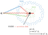 |
Fig. 1. Schematic view of the relative location and size of the different regions of a quasar and illustration of the reverberation effect. RS is the Schwarzschild radius of the central SMBH. The continuum light from the central accretion disk (red) is reverberated both in the BLR (green) and in the NLR (blue), which are much larger than the accretion disk and are therefore much less affected by microlensing (see Sect. 3.3). |
As the BLRs and accretion disks of quasars are generally smaller than 10−1 pc (Mosquera & Kochanek 2011), these regions are not spatially resolved by any existing instrument1, and several techniques have been developed to infer the structure of the BLR and the accretion disk indirectly. The first measurements of the sizes of accretion disks were derived from the flux–size estimate, which relies on the relation between the luminosity and radius of the accretion disk, R0, given by the thin-disk model and following R0 ∝ L1/3 (Collin et al. 2002; Morgan et al. 2010). Using this approach, Mosquera & Kochanek (2011) predicted the radii of accretion disks in 87 strongly lensed quasars. Alternatively, continuum reverberation mapping, that is, the measurement of the time-lag between different parts of the continuum, has been used to estimate the size of the accretion disk under the assumption of the lamp-post model (e.g., Krolik et al. 1991; Chan et al. 2020). Examples of such measurements of quasar accretion disks in non-lensed quasars can be found in Mudd et al. (2018), Homayouni et al. (2019), and Yu et al. (2020). As for the BLR size measurement, the reverberation mapping technique (Blandford & McKee 1982) relies on the time-lag between the light rays coming straight from the accretion disk and those scattered (reverberated) by the BLR, as shown in Fig. 1. This method has been used to measure the size of the BLR and infer the mass of the SMBH through spectrophotometric monitoring (e.g., Bentz et al. 2009; Du et al. 2016; Williams et al. 2021; Kaspi et al. 2021).
A complementary and independent approach to studying quasar structure is to use microlensing by stars in the lensing galaxy of strongly lensed quasars (Chang & Refsdal 1979). In any given strongly lensed quasar, stars passing in front of the lensed images split the wavefronts of the incoming light, creating additional micro-images of the source separated by a few micro-arcseconds. The image splitting is not observable with existing instrumentation, but the resulting microlensing magnification is. In practise, the relative motion between observer, lens, microlenses, and source induces a flickering of the macro-lensed observable images. This flickering acts over timescales of weeks to years (e.g., Mosquera & Kochanek 2011) and is a nuisance when measuring time delays (e.g., Tewes et al. 2013; Millon et al. 2020b) or macro-magnification ratios between the quasar images (Blackburne et al. 2006). However, because the variable micro-magnification depends on the dimensions of the source, it also presents an opportunity to measure the size and energy profile of accretion disks (Eigenbrod et al. 2008b) and to study quasar structure in general. Microlensing techniques are mainly sensitive to the half-light radius of the source and are less sensitive to the shape of its light profile (Mortonson et al. 2005; Vernardos & Tsagkatakis 2019).
The apparent radius of an accretion disk is wavelength dependent because its inner region is hotter than its outskirts and therefore emits more energy (Shakura & Sunyaev 1973). As a consequence, the micro-magnification, which depends on the size of the source, depends on the wavelength of observation as well, even though microlensing is by nature achromatic. This leads to chromatic flux ratios between the observed images of a strongly lensed quasar, which have been identified in spectrophotometric monitoring data (e.g., Eigenbrod et al. 2008a). Such chromaticity also enables the measurement of quasar accretion disks through single-epoch multi-wavelength observations (Bate et al. 2008), and although this method may be biased by the strength of the wavelength-dependent microlensing, it is a reliable way to measure the sizes of accretion disks (Bate et al. 2018). While in many strongly lensed quasars this method yields results in agreement with the thin-disk theory (e.g., Bate et al. 2008; Floyd et al. 2009; Mediavilla et al. 2011; Rojas et al. 2014), in other systems it was found that the thin-disk model underestimates the size of the accretion disk by up to an order or magnitude (e.g., Blackburne et al. 2011; Motta et al. 2017; Bate et al. 2018; Rojas et al. 2020), which according to Cornachione & Morgan (2020) would favour shallower accretion disk temperature profiles than predicted by the thin-disk model.
A second approach to measuring quasar structure with microlensing is to use the pair-wise difference light curves between quasar images corrected for the time-delay and macro-magnification – often called ‘microlensing light curves’ – as they are assumed to be corrected for intrinsic quasar variations by construction. Currently, most methods currently in use interpret such pair-wise differences in light curves by following the fitting technique introduced by Kochanek (2004). This latter consists of a Monte Carlo analysis comparing huge amounts of simulated microlensing light curves (∼1011) generated by varying a number of physical parameters on quasar structure, microlensing, and velocities until a fit to the data is obtained. The main limitation of this approach is that, as the microlensing light curves get longer, their complexity grows because of the inclusion of more microlensing events, and consequently the number of simulations required to fit the data rises drastically. In addition, this method assumes that microlensing occurs over long timescales, of the order of years, and focuses on the long-term effects while overlooking short-term variability. As a consequence, features shorter than ∼1 year have much less weight in the final inference than the longer features, resulting in a frequency filtering of the microlensing signal that may lead to overestimation of the disk size2. Measuring the disk size with this technique has been achieved by a number of authors (Morgan et al. 2008, 2012, 2018; Cornachione et al. 2020b). By comparing their microlensing measurements with luminosity-based ones, Morgan et al. (2010) and Cornachione et al. (2020b) pointed out a systematic discrepancy, which they explain by a possible shallower temperature profile of the disk than predicted by the thin-disk model. Finally, a novel approach to microlensing light curve analysis was introduced by Vernardos & Tsagkatakis (2019), who employ machine learning to measure the accretion disk size. Such an approach has the potential to capture both long- and short-term (low- and high-frequency) variability in the signal, but has not yet been applied to data.
High-frequency variations are visible in high-cadence monitoring campaigns of strongly lensed quasars (e.g., Millon et al. 2020a), potentially carrying valuable information on quasar structure, but their analysis is not possible with the light-curve-fitting method because of the previously mentioned flaws. In addition, high-frequency signals can be introduced either by microlensing or can be partly due to reverberation processes occurring between the inner accretion region and the BLR (e.g., see Fig. 1). The characteristics of the high-frequency variations depend on the relative sizes of the accretion disk and the BLR and lead to the so-called ‘microlensing-aided reverberation’ first suggested by Sluse & Tewes (2014). In the present work we consider this effect for the first time in the analysis of real data.
In order to study high-frequency variations, we introduce a new method that relies on the Fourier power spectrum of the microlensing light curve, which allows us to characterise the overall properties of the observed signal rather than any specific realisation of the light curve. Fitting the power spectrum enables us to investigate every timescale of variation, both in the high and low frequencies in a computationally tractable way. The method is applied to the light curve of QJ 0158-4325, previously studied by Morgan et al. (2012) using the light-curve-fitting method, who estimated a significantly larger disk size than that obtained by Mosquera & Kochanek (2011) using a flux-based source size. As we show in our study, the power spectrum method demonstrates that part of the high-frequency variation in the microlensing light curve can be explained by continuum light being reverberated in the BLR. For the first time, we estimate the size of the BLR via microlensing-aided reverberation.
The paper is organised as follows: Sect. 2 explains how the microlensing light curve of QJ 0158-4325 is obtained, together with its power spectrum. Section 3 describes our new power-spectrum analysis approach. Section 4 explains the validation process of the method as well as the constraints obtained on the structure of the quasar with and without taking into account the reverberation process. We conclude with a discussion of our results in Sect. 5. Throughout this work we assume Ωm = 0.3, ΩΛ = 0.7, and H0 = 72 km s−1 Mpc−1.
2. Data
QJ 0158-4325 is a doubly imaged quasar (see Fig. 2) discovered by Morgan et al. (1999) that has been monitored for 13 years by the Leonhard Euler 1.2m Swiss Telescope in the context of the COSmological MOnitoring of GRAvItational Lenses (COSMOGRAIL) program (Courbin et al. 2005; Eigenbrod et al. 2005). In Millon et al. (2020b), the light curves of this object were extracted following three main steps: first, the instrumental noise and the sky level were subtracted; then a point spread function (PSF) estimated from nearby stars was fitted to each quasar image; before the flux was extracted at the image position with the MCS deconvolution algorithm (Magain et al. 1998; Cantale et al. 2016). This procedure allows one to extract the individual fluxes of the quasar images decontaminated from the light of the lensing galaxy (see Millon et al. 2020b, for more details). The resulting light curves of QJ 0158-4325 are shown in Fig. 3.
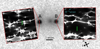 |
Fig. 2. QJ 0158-4325 observed with the Hubble Space Telescope in the F814W filter (program ID 9267; PI: Beckwith). The microlensing magnification maps (corresponding to ⟨M⟩ = 0.3 M⊙) are shown for each quasar image using the same colour scale, and are rotated with respect to the shear angle. The green line indicates a realisation of a trajectory of the source, the same in orientation and length for both maps drawn from the probability density function of ve shown on Fig. 5. |
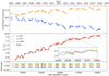 |
Fig. 3. Top: COSMOGRAIL R-band light curves of images A and B of QJ 0158-4325 over a period of 13 years. For clarity, the B curve has been artificially shifted upwards by 0.2 mag (adapted from Millon et al. 2020b). Middle: microlensing light curve (red) obtained from the observations using Eq. (2) with ΔtAB = 22.7 days (Millon et al. 2020b), along with examples of spline fitting with different values of the η parameter (defined in Sect. 2.2). Bottom: residuals of the three illustrative spline fits to the microlensing light curve. The number on the left indicates the artificial shifts applied for the purpose of clarity. |
2.1. Microlensing light curve
The observed light curve of a quasar image, Sα(t), in magnitudes is the sum of the macro-magnification, ℳα, the intrinsic variation in each image, Vα(t), and the microlensing magnification mα(t):
 (1)
(1)
Without loss of generality, we can assume that the signal of image B of QJ 0158-4325 is simply a time-shifted version of image A, that is, VB(t) = VA(t − ΔtAB), where ΔtAB is the time-delay between the two images. Hence, the microlensing signal can be found by subtracting the observed light curves after correcting for the time-delay and macro-magnification:
 (2)
(2)
We note that we refer to this signal as ‘microlensing’ but it can well include a fraction of non-microlensed continuum light from the BLR, as shown below. This microlensing curve should therefore be seen as containing any ‘extrinsic’ variations, that is, variations unrelated to the quasar instrinsic variability. We keep the macro-magnification constant across the length of the light curve as we assume that it only changes on much longer timescales (see Table 1 for the values used in this work).
As detailed in Millon et al. (2020b), the determination of ΔtAB is done by fitting the observed light curves with free-knot splines implemented in the PyCS package (Millon et al. 2020c). Such splines are piece-wise polynomials with the mean distance between two knots assigned by a parameter η which controls the smoothness of the resulting fit. Free-knot splines allow the positions of the knots to be adjusted so that they capture both long and short features in the data being fitted. A single free-knot spline is fitted simultaneously to all light curves to model the intrinsic variation of the quasar while additional splines model the extrinsic (microlensing) variations in each light curve separately. A simultaneous fit of all instrinsic and extrinsic splines then allows us to adjust the time delays.
For QJ 0158-4325, the time-delay was found to be ΔtAB = 22.7 ± 3.6 days (Millon et al. 2020b) and the resulting microlensing light curve (Eq. (2)) is shown in the middle panel of Fig. 3. We do not expect the uncertainty on the time-delay to alter our constraints on the quasar structure because it is much smaller than the shortest timescale of interest, as discussed below. In the present study, we focus on features in the differential light curve that are longer than 100 days. The microlensing signal shows a steady rise throughout the period of observations, resulting in an overall increase of ≈1.2 mag, on top of which short modulations are observed within a single season; small-scale variations are seen in the first seven seasons (from 2005 to 2011) with a typical peak-to-peak amplitude of 0.1 magnitudes. Among the many lensed quasars monitored by the COSMOGRAIL project, very few exhibit such rich and diverse microlensing and/or extrinsic behaviour. QJ 0158-4325 is therefore a promising test bench for investigating both high- and low-frequency variability.
2.2. Power spectrum of the microlensing light curve
We represent the data in Fourier space in order to capture the high-frequency features that are missed by the light-curve-fitting method applied to QJ 0158-4325 in Morgan et al. (2012). The resulting power spectrum therefore holds information across all the frequencies and allows us to treat high- and low-frequency signals simultaneously. In the following, we compute power spectra of both observed and simulated light curves using a standard Fourier transform. To tackle the so-called spectral leakage problem (Harris 1978), that is, the spurious broadening of spectral lines in frequencies for which the length of the signal is not a multiple of the corresponding period, we use a standard flat-top window function.
As shown in the upper panel of Fig. 3, the light curves are not evenly sampled: within a season, two measurements may be separated by three or four days, and season gaps prevent the signal from being evenly sampled throughout the entire curve. The latter would in fact introduce a pattern in the Fourier transform that can be mistakenly interpreted as a periodic signal. To mitigate this, we interpolate the data through the season gaps using the continuous spline that resulted from the fitting technique to measure the time-delays, as outlined above. This offers a flexible and model-independent way to fit time-series. We set the sampling rate to one day and then compute the power spectrum.
The resulting power spectra have two main sources of uncertainty: on one hand, the photometric uncertainties of the raw data induce uncertainty in the very high frequencies corresponding to the sampling rate of the light curve (of the order of 1-10 days). On the other hand, the choice of the parameter η can have a significant impact on the fitting of short-timescale variations because, as illustrated in the middle panel of Fig. 3, features shorter than η are filtered out. The difference between underfitting and overfitting the data depends on the origin we attribute to a given short-timescale variation and whether we want to discard it or not. As we aim to use as few hypotheses as possible on the nature of these short variations, we do not make any assumption on the actual value of η but rather consider a plausible range in order to estimate the uncertainty induced by this parameter. We define this range as [30:100] days in order that it be superior to the time sampling of the data while still capturing most of the high-frequency features. The scatter of the residuals in the bottom panel of Fig. 3 shows that the selected range smoothly fits the data and most of the high-frequency variability is accounted for.
In order to quantify the uncertainty on the power spectrum induced by these effects, 1000 different realisations of photometric noise are produced for every value of η sampling the range [30:100] days with steps of 5 days used for the spline fitting, yielding a set of 14000 data-like light curves. The power spectrum of the data that will be used further in this study is given by the mean and standard deviation of this set of light curves, shown in Fig. 4. As the extreme values of η either overfit or underfit the light curve, the resulting uncertainty is conservative. We note that the relative uncertainties are negligible up to frequencies of 10−2 days−1. For higher frequencies, the power drops below 10−3 and the relative uncertainties diverge because of the two aforementioned sources of uncertainty. As the Einstein crossing time is around 18 years in the QJ 0158-4325 system (Mosquera & Kochanek 2011), we do not expect the light curve to contain features with timescales shorter than 100 days. As a result, there should not be a significant amount of signal above the 10−2 days−1 threshold and the power present in these frequencies is induced by photometric noise. Therefore, we exclude the frequencies above 10−2 days−1 (i.e. features shorter than 100 days) from the following analysis.
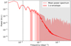 |
Fig. 4. Power spectrum of the observed microlensing light curve computed as the mean of the power spectra obtained for 1000 different realisations of photometric noise for every value of η sampling the range [30:100] days with steps of 5 days used for the spline fitting parameter (see text). The 1−σ envelope is given by the standard deviation of the same set of power spectra. The dashed black line marks the boundary between low and high frequency and the grey area indicates our adopted frequency limit of 10−2 days−1, below which photometric uncertainties dominate the data. |
3. Methods
In this section, the procedure of generating simulated light curves is described, as well as the way the simulated and observed power spectra are compared. The simulated variable flux of a quasar image, Fα(t), is assumed to be the combination of three components (Sluse & Tewes 2014): the intrinsic flux variability, I(t), due to the stochastic emissions of the accretion disk; the microlensing magnification, μ(t), due to stars in the lens galaxy; and the flux arising from the BLR, FBLR(t), which echoes the intrinsic variability of the continuum light of the accretion disk. As the BLR is much larger than the accretion disk (typically ten times larger, Mosquera & Kochanek 2011), microlensing of the resulting reverberated light is expected to be small3. Hence we have:
 (3)
(3)
where μα is the time-dependent microlensing magnification and Mα is the constant macro-magnification. Each component in this equation is separately described below.
3.1. Intrinsic variability
The variability of the accretion disk is commonly described by a damped random walk model (Kelly & Siemiginowska 2009; MacLeod et al. 2010; Ivezić & MacLeod 2013). As the variability of QJ 0158-4325 shows no major deviation from the standard quasar optical variability, we model it using a damped random walk model parametrized by a characteristic timescale, τDRW, and amplitude, σDRW, of the variations. We use the JAVELIN code presented by Zu et al. (2013) to create simulations of intrinsic light curves, which are designed for studying the variability of quasars (Zu et al. 2011). A damped random walk consists of a Gaussian Process, 𝒢𝒫, with mean intensity  and covariance Cov(Δt) between two moments in time separated by Δt such that:
![Mathematical equation: $$ \begin{aligned} I(t) = \mathcal{GP} \left[\overline{I},Cov(\Delta t)\right], \end{aligned} $$](/articles/aa/full_html/2022/03/aa41808-21/aa41808-21-eq7.gif) (4)
(4)
with the covariance given by :
 (5)
(5)
Knowing τDRW and σDRW completely defines the 𝒢𝒫, from which different but equivalent realisations of the intrinsic light curve can be drawn.
3.2. Microlensing variability
Magnification maps are used to simulate microlensing events produced by a given population of stars in the lens galaxy. In order to simulate a stellar population, we need to compute the values of the convergence, κ, the stellar surface density, κ*, and the shear, γ, at each image location from the smooth model of the lens galaxy mass distribution (i.e. macro-model; see Sect. 4 and Table 1). We then use a Salpeter initial mass function (IMF) to describe the stellar mass distribution around a given mean stellar mass ⟨M⟩. The maps are generated with the GPU-D software, which implements the direct inverse ray-shooting method as described in Vernardos et al. (2015), used in other microlensing studies as well (e.g., Chan et al. 2021).
The characteristic scale of the magnification patterns created by such compact objects in the lens galaxy is their Einstein radius, RE, defined in the source plane as:
 (6)
(6)
where G is the gravitational constant, c the speed of light, and Dl, Ds, and Dls correspond to the angular diameter distances from the observer to the lens, from the observer to the source, and from the lens to the source, respectively. The map dimensions are 8192 × 8192 pixels, corresponding to a physical size of 20RE × 20 RE and a pixel size of 0.0024 RE. Figure 2 shows the configuration of the QJ 0158-4325 lens system along with a realisation of magnification maps corresponding to the κ, κ*, and γ given by the smooth mass model at the given quasar image positions.
In order to study the magnification of a finite-sized source by a given caustic, we need to assume a light distribution projected on the plane of the sky. The accretion disk of the source is assumed to be described by the thin-disk model (Shakura & Sunyaev 1973), in which a monochromatic light profile as a function of radius is given by:
![Mathematical equation: $$ \begin{aligned}&I_{0}(R) \propto [\exp (\xi ) -1]^{-1} , \quad \mathrm{where} \\&\xi = \left(\frac{R}{R_{0}}\right)^{3/4}\left(1-\sqrt{\frac{R_{\rm in}}{R}} \right)^{-1/4}, \nonumber \end{aligned} $$](/articles/aa/full_html/2022/03/aa41808-21/aa41808-21-eq10.gif) (7)
(7)
with R0 being the scale radius, that is, the radius at which the temperature matches the rest-frame wavelength of the observation assuming black body radiation, and Rin < R is the inner edge of the disk. Here we assume Rin = 04 and we explore a range of R0 values that contains the value estimated by Mosquera & Kochanek (2011), i.e. R0 ≈ 0.067 × RE (in the case of ⟨M⟩ = 0.3 M⊙), which is ≈15 pixels on the maps that we use. To compute the magnification induced on the source, we need to convolve the magnification map with the light profile.
The timescale of a microlensing event is set by the effective velocity in the source plane, ve, which is the vectorial sum of the transverse velocities of the microlenses, v*, of the lens galaxy vl, of the source, vs, and of the observer, vo. As described in Neira et al. (2020), the direction of the microlense velocity is random and is uniformly sampled in the [0;2π] interval. The magnitude of this velocity vector is given by:
 (8)
(8)
where ϵ is a factor depending on κ and γ, and is assumed to be 1 (Kochanek 2004), and σ* is the velocity dispersion at the lens galaxy centre. The directions of vl and vs are random and their magnitude is drawn from a Gaussian distribution with a given standard deviation, σpec(z), as a function of redshift. Therefore, these can be combined into a single normal variable vg with a random direction and a magnitude given by a Gaussian with a standard deviation given by:
 (9)
(9)
The velocity of the observer is measured with respect to the cosmic microwave background velocity dipole:
 (10)
(10)
where vCMB is the measured velocity vector with respect to the cosmic microwave background, and  the line of sight of the observer. The magnitude and direction of this component are computed using the position of the object on the plane of the sky. Combining these terms, the effective velocity is:
 (11)
(11)
In the case of QJ 0158-4325, zl = 0.317 and zs = 1.29 (Chen et al. 2012). All other relevant parameters for QJ 0158-4325 are given in Table 1 and the resulting probability distribution of ve from which the effective velocity in the source plane is drawn is shown in Fig. 5. The probability density function in Fig. 5 is approximated by a Gaussian kernel density estimator and then sampled through the inverse transform sampling method.
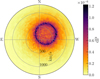 |
Fig. 5. Probability density of the effective velocity, ve, in the source plane for QJ 0158-4325 from Eq. (11). |
3.3. Reverberated variability
As shown in Sluse & Tewes (2014), delayed reverberation of the continuum light from the BLR can significantly alter the observed microlensing signal with modulations on short timescales. In the case of QJ 0158-4325, Faure et al. (2009) showed that the Mg II as well as the Fe II spectral lines, both arising from the BLR, fall into the R-band used in this work. It therefore makes sense to consider continuum reverberation as a mechanism contributing to the observed light curves.
We can describe the reverberation component in Eq. (3) as FBLR(t) = fBLRr(t), where fBLR is the flux ratio between the line and the continuum and r(t) is the reverberated flux. The latter can be computed as a convolution, r(t) = Ψ(t, τ)*I(t), between the intrinsic signal, I(t), and Ψ(t, τ), a time-lagging transfer function that depends on the radius of the BLR through a corresponding time lag τ = RBLR/c. Equation (3) then becomes:
![Mathematical equation: $$ \begin{aligned} F_{\alpha }(t) = M_{\alpha } \mu _{\alpha }(t) I(t) + M_{\alpha } f_{\rm BLR}\left[\Psi (t,\tau )*I(t)\right]. \end{aligned} $$](/articles/aa/full_html/2022/03/aa41808-21/aa41808-21-eq16.gif) (12)
(12)
In this work we model the reverberation region as a diffuse ionised gas cloud with the geometry of a thin shell (Peterson et al. 1993), so that Ψ(t, τ) is a top hat kernel with an amplitude A and a width equal to twice the assumed time-lag τ:
 (13)
(13)
The values of the fBLR and RBLR parameters examined here are given in Table 1.
3.4. Light-curve simulation and fitting
Combining all the above model components, we are now able to simulate light curves for each quasar image using Eq. (12). The free parameters are ⟨M⟩, ve, R0, σDRW, and RBLR, which we refer to as vector ζ. The final light curve to be compared to the data is obtained by dividing (subtracting) the flux (magnitudes) of pairs of simulated light curves for images A and B. Examples of simulated light curves with and without reverberation along with their corresponding power spectra are shown in Fig. 6.
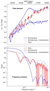 |
Fig. 6. Top panel: example of a simulated light curve with and without reverberation (dotted and solid lines respectively). Bottom panel: corresponding power spectra. The curves and power spectra have been produced using ⟨M⟩ = 0.3 M⊙, ve = 1236 km s−1, R0 = 0.5RMK11, σDRW = 30 and RBLR = RBLRMK11. Adding reverberation clearly adds power to the high-frequency part of the spectrum. |
For any given ζ, a batch of 105 curves is created from the magnification maps and their power spectrum is computed. The mean Psim(ω) and standard deviation σsim(ω) of the power spectrum in each frequency bin are then compared to the data using a chi-square statistic:
 (14)
(14)
where Pdata(ω) is the mean power spectrum of the data at the frequency ω and σdata(ω) its standard deviation shown in Fig. 4. This can be turned into a likelihood through:
 (15)
(15)
Eventually, the posterior probability is obtained using Bayes theorem:
 (16)
(16)
where 𝒫(ζ) is the prior probability of the parameters ζ and E(d) is the probability of the data, that is, the Bayesian evidence. Calculating E(d) requires integration of the posterior across the whole parameter space, which is beyond the computational limits of this study. This means that we cannot compare different models, but we can still use relative probabilities within any given model. All parameters are assumed to have a uniform prior except ve, whose prior is given in Eq. (11). Finally, we obtain the posterior probability marginalised over a given parameter or subset of parameters ζi through:
 (17)
(17)
4. Results
We studied the effect of high-frequency variability, such as that introduced by a reverberated BLR component, when measuring the size of the accretion disk. In doing so, we found a new way to measure the size of the BLR using the microlensing light curves from Eq. (2) in the full frequency range. Before describing our results, we present our prior assumptions for the various model parameters listed in Table 1.
Intrinsic variability. The long-term brightness decrease of image B (see Fig. 3) compared to the behaviour of the light curve A, which consists of oscillations around a mean, suggests two possible scenarios: the intrinsic luminosity of the quasar is decreasing and image A is microlensed or the intrinsic luminosity of the quasar is rather constant and a microlensing event which started in image B before the beginning of the observations is now ending, leading to a decrease in the micro-magnification. According to MacLeod et al. (2016), photometric changes of |Δm|≥1 mag over ≈10 years, such as those observed in light curve B, are very rare (around 1% of quasars display this kind of variability). Furthermore, spectra of QJ 0158-4325 shown in Faure et al. (2009) (i.e. taken during the first quarter of the light curve of Fig. 3), show a typical Type 1 QSO spectrum for image A whereas the B spectrum shows faint and deformed emission lines. Altogether, these observations lead us to favour the second scenario. We therefore consider image A to be microlensing-free, and use its light curve as a proxy for the quasar intrinsic variability. Using the JAVELIN software (Zu et al. 2013), which employs a maximum likelihood approach in a Markov chain Monte Carlo (MCMC) framework, we find τDRW = 810 days for the assumed damped random walk intrinsic variability model. However, the observed light curve is the result of a convolution between the driving source and the light profile of the quasar. Therefore, the amplitude of the variations, σDRW, cannot be constrained, because it is degenerate with the radius of the source R0 which is also unknown in this study. A large interval is therefore considered for exploring this parameter, which includes the values of σDRW for all the known quasars (Suberlak et al. 2021).
Lens-mass model and magnification maps. Morgan et al. (2012) explore a list of lens-mass models with a stellar mass fraction, fM/L, of between 0.1 and 1, and give a relation between fM/L and the time-delay between the two images Δt. Using this relation and the time-delay measured by Millon et al. (2020b), we obtain fM/L = 0.9, which we use throughout the following. We adopt the κ, γ, and κ* values at image locations from Morgan et al. (2008), also listed in Table 1, to compute the magnification maps that we use below. As model uncertainties are not given, we assume δκ, δγ ≤ 0.01, as quoted in most modelling works (e.g., see Table B1 of Wong et al. 2017). According to Vernardos & Fluke (2014), magnification maps within these uncertainties have a statistically equivalent magnification probability distribution. As a sanity check, the same experiment was performed with a different mass model with Δκ, Δγ ≥ 0.03 leading to the same general conclusions. We therefore do not expect the uncertainty on the macro-model to influence our study.
In most microlensing light-curve-fitting studies (Kochanek 2004; Morgan et al. 2008; Cornachione et al. 2020b), ⟨M⟩ = 0.3 M⊙ is taken as a reference mass around which a range of mean mass is explored. Because we are interested in high-frequency variability, we also explore the effect of smaller values of the mean mass, that is, ⟨M⟩ = 0.1 M⊙ and ⟨M⟩ = 0.01 M⊙, which can introduce shorter microlensing events for any given effective velocity due to the corresponding small physical size of the caustics. Choosing a shallower Chabrier IMF instead of the steeper Salpeter one used here leads to fewer low-mass microlenses and therefore reduces any effect of high-frequency variability. Although this has been shown to affect magnification map properties (see Chan et al. 2021), our goal here is to understand such short-timescale variability and therefore we use the Salpeter IMF for all values of ⟨M⟩.
Accretion disk size. In order to limit the number of free parameters of our study, we assume a face-on thin-disk model. The expected maximal inclination angle of a type-I AGN is ∼60 degrees with respect to the line of sight (e.g., Borguet et al. 2008; Poindexter & Kochanek 2010) and can induce, at most, a factor two systematic effect on the determination of R0. Nevertheless, R0, ve, and the inclination angle are degenerate. We therefore repeated our measurement of RBLR each time varying R0 and ve by factors of several and found no significant differences from our results in the face-on disk assumption. We use log(R0/cm) = 15.07 ≡ RMK11 from Mosquera & Kochanek (2011) as a reference value for the scale radius. We explore R0 in the range 0.1 − 6 × RMK11, which is bound at the low end by the magnification map resolution and extends high enough to include the measurement of Morgan et al. (2012).
Reverberated variability. As mentioned previously, microlensing is dominant in image B compared to image A. Therefore we use the spectrum from image A to derive fBLR in order to avoid any contamination from a possibly microlensed continuum. To do so, the spectrum presented in Faure et al. (2009) was analysed using a multi-component decomposition as in Sluse et al. (2012). However, contrary to Sluse et al. (2012), a MCMC approach was used to estimate the median fBLR and a 68% credible interval (see Table 1). We emphasise the fact that fBLR is computed as the fraction of flux coming from the BLR compared to the continuum in the R-band, irrespective of the atomic species, and therefore both the Mg II and Fe II emissions are included. As for the radius of the BLR, Mosquera & Kochanek (2011) used the Hβ-BLR size–luminosity relationship (Bentz et al. 2009) to estimate RBLR = 1.71 × 1017 cm ≈ 39 light days, which we adopt here as our reference value, RBLRMK11. The lower bound of the RBLR range that we explore is 0.1 × RBLRMK11 ≈ 5 light days, which is the smallest reverberation delay observable with the sampling of the light curve set to one point every 2–3 days. The upper bound is set to 2.5 × RBLRMK11 to include the confidence interval of the Mosquera & Kochanek (2011) estimate.
To understand the effect of key parameters in the frequency of the signal in the simulated light curves we provide an illustrative example in Fig. 7, where we show power spectra calculated for different values of the transverse velocity, ve with corresponding directions drawn from the probability density function shown in Fig. 5, and the scale radius, R0, two of the main free parameters in subsequent models. Firstly, we note that for a given value of R0 the power has a tendency to increase with ve, which is justified because, the higher the velocity, the faster the source crosses caustics, inducing more high-magnification events in both the high and low frequencies. Secondly, for a given value of ve, the power in the high frequencies is inversely proportional to R0. This is explained by the microlenses magnifying an ever decreasing portion of larger accretion disks, with the resulting magnification effect being diluted within the overall flux, leading to smoother and weaker high-frequency variations.
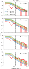 |
Fig. 7. Mean (lines) and upper 1−σ envelope (shaded area) of power spectra from 100 000 simulated curves for different (ve, R0) configurations, in the absence of reverberation (FBLR = 0 in Eq. (3)), compared to the data (same as Fig. 4). Due to the logarithmic scale, the lower envelopes extend almost to the x-axis and are not displayed for clarity. The vertical dashed line marks the boundary between low and high frequency. |
Furthermore, Fig. 7 shows that in the low frequency regime the models match reasonably well the data, while most of the model differences occur in the high frequencies. It is almost impossible to simultaneously match both the low and high frequencies, whatever the model parameters may be. This suggests that other physical mechanisms might be at play, in addition to microlensing, which we explore with the following three experiments:
-
Low frequency (LF): we apply the power spectrum method in the same setup as that used by Morgan et al. (2012), that is, we use only the low-frequency part of the power spectrum, imposing a cutoff at 1/750 days−1 that corresponds to the typical timescale considered in Fig. 2 of Morgan et al. (2012). At this stage, we do not include any reverberation signal and set FBLR = 0 in Eq. (3). As a result, even though intrinsic variability is included in this model, it is cancelled out because we are studying the differential microlensing light curves. This model is therefore not sensitive to the intrinsic variability parameters σDRW and τDRW.
-
Full frequency (FF): we perform the same analysis as above, this time including the high frequencies up to 1/100 days−1.
-
Reverberation full frequency (RFF): we use the full frequency range of the data, as in the FF model, but this time we include the reverberation of the continuum.
The details and outcomes of each experimental setup are detailed below.
4.1. LF: Low frequencies without reverberation
In Morgan et al. (2012), the shortest features in the light curves last approximately two consecutive seasons, or ≈750 days (see their Fig. 2). This translates into frequencies of up to 1/750 days−1, which is lower than the 1/100 days−1 limit that we set in Sect. 2. We therefore adopt 1/750 days−1 as being our boundary between what we define as low and high frequency. Here, we model only the low-frequency power spectrum of the data, which contains by design the same signal frequencies as the data used in Morgan et al. (2012).
The top row of Fig. 8 shows the posterior probability from Eq. (16) as a function of ve, R0, and ⟨M⟩. The distribution of R0 broadens with decreasing ⟨M⟩, becoming almost uniform for the smallest mean mass of ⟨M⟩ = 0.01 M⊙, and therefore not providing any useful constraint. This can be understood in terms of the physical size of the magnification maps, which depends on ⟨M⟩ through the Einstein radius of the microlenses, RE (see Eq. (6) and Table 1), with respect to the velocity: decreasing ⟨M⟩ is equivalent to rescaling the magnification map to a smaller physical size that allows the source to cross the map more rapidly for the same effective velocity (which is equivalent to increasing the effective velocity while keeping the mass fixed). Thus, small masses and larger radii can induce enough high-frequency power to fit the data as well as the smaller radii and larger masses.
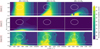 |
Fig. 8. Slices of the marginalised posterior probability of the (ve, R0, ⟨M⟩) parameter space (three-dimensional after the marginalisation over the angle of ve using Eq. (17)) for each of the three models described in Sect. 4. Model LF: light curves simulated without reverberation and fitted only to the low-frequency data, i.e. up to 1/750 days−1, which corresponds to the same frequency cut as in Morgan et al. (2012). Model FF: same simulations are fitted to the full frequency range, i.e. up to 1/100 days−1. Model RFF: light curves are now simulated with reverberation (fBLR = 0.432 ± 0.036, σDRW = 55 and RBLR = RBLRMK11) and the full observed frequency range up to 1/100 days−1 is considered. The solid line corresponds to RMK11, the estimate of Mosquera & Kochanek (2011), the ellipse represents the (ve, R0) measurement interval from Morgan et al. (2012). The coloured contours encapsulate [10–100]% of the probability volume and are projected in each of the displayed slices. We note that our probability densities are not scaled by the evidence and therefore cannot be compared across different models. |
Overall, our power spectrum measurement is in good agreement with the estimate of Mosquera & Kochanek (2011), while it is consistent within 1 to 2σ with the result of Morgan et al. (2012) in the ⟨M⟩ = 0.01 − 0.1 M⊙ cases. In the ⟨M⟩ = 0.3 M⊙ case, we note a slight discrepancy with the results of Morgan et al. (2012). This can be explained by our use of longer light curves (6 more seasons) and the use of a model-driven prior on the angle of ve, as illustrated in Fig. 5, instead of the uniform prior used in previous studies5. Model LF is a sanity check demonstrating that, when restricted to low frequencies, the power spectrum and light-curve-fitting methods give compatible results and the data can be explained by microlensing alone.
4.2. FF: Full frequency range without reverberation
We now include the high-frequency signal in the data and attempt to explain it assuming that the observed variations come solely from microlensing of the accretion disk, that is, exactly the same model as in the LF setup. Our results, shown in the second row of Fig. 8, favour much smaller accretion disks with R0 < 0.5RMK11, excluding both the result of Morgan et al. (2012) and the estimation of Mosquera & Kochanek (2011). This is less prominent for the case with ⟨M⟩ = 0.01 M⊙, where we observe the same behaviour for larger R0 as in the LF case, extending the compatible sizes to somewhat larger values. Clearly, microlensing alone has problems in explaining the high-frequency signal and we need to invoke additional sources of variability to explain the data, as we do in the following case.
4.3. RFF: Full frequency range with reverberation
Adding the reverberation process to the simulated light curves is expected to increase the power of the high frequencies in the signal. In the bottom row of Fig. 8 we show the posterior probability as a function of ve, R0, and ⟨M⟩ for a fiducial reverberation model with RBLR = RBLRMK11 and σDRW = 55 (see also Fig. 10 and Sect. 4.4 ).
As we can see in the third row of Fig. 8, when including the reverberation effect, the constraint obtained for the radius of the accretion disk R0 is now dominated by the prior on ve and R0 for every ⟨M⟩ explored. Still, we note that the areas corresponding to any given percentage of enclosed posterior probability shrink with the value of ⟨M⟩. Indeed, if a simulated power spectrum is compatible with the data for ⟨M⟩ = 0.3 M⊙, the addition of power induced by the decrease in ⟨M⟩ (as discussed in Sect. 4.1) pulls the simulated power spectrum away from the data, thereby reducing their compatibility. Therefore, this model tends to favour the standard value of ⟨M⟩ = 0.3 M⊙.
4.4. RBLR measurement
In order to measure the size of the reverberating region, RBLR, we first explore the effect of the amplitude of the intrinsic variability, σDRW, and of RBLR on the simulated power spectra, while keeping the microlensing parameters fixed at ⟨M⟩ = 0.3 M⊙, R0 = RMK11, and ve = 700 km s−1. The use of ⟨M⟩ = 0.3 M⊙ is motivated by the fact that galaxies are unlikely to host a population of objects with ⟨M⟩ = 0.1 or 0.01 M⊙ (see Sect. 4.3). Including reverberation in the analysis allows us to explain the high frequency using a realistic value of ⟨M⟩, or at least a consensus one. As for ve, we use a value close to the mean value from Eq. (11) (see also Table 1 and Fig. 5). We stress the fact that, if the microlensing is identical in both images (i.e. μA(t) = μB(t) in Eq. (3), which is more likely to happen if both images are not microlensed), the effect of reverberation is absent from the differential light curve we analyse. Therefore, reverberation is not a stand-alone part of this study and the reverberation-induced variability ends up being weighted as a function of time because of microlensing in the differential light curve. Figure 9 shows that increasing σDRW leads to more power at the high frequencies, mostly because the now stronger intrinsic variations are reverberated after a time-lag (τ = RBLR/c, see Eq. (13)) of the order of tens to hundreds of days, i.e. with a frequency > 1/750 days−1. Analysing the effect of the BLR size, RBLR, is more complex. For a given transfer function, Ψ(t, RBLR/c), a short variation of typically ≈100 days in the intrinsic signal I(t) appears twice in light curves simulated using Eq. (3): once at time t and a second time at t + RBLR/c. As RBLR is increased, the echoed signal moves further, eventually becoming fully separated spatially from the one originating at the disk, and is seen as a whole new feature of the light curve. This adds power to the high-frequency domain, justifying the difference between the RBLR = 0.2RBLRMK11 and RBLR = RBLRMK11 cases in Fig. 9. As we keep increasing RBLR, Ψ(t, RBLR/c) gets wider and starts to smooth out the short intrinsic variations, reducing their power. This explains the drop in power in the highest of the frequencies when considering the highest values of RBLR in Fig. 9.
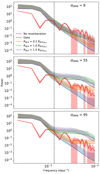 |
Fig. 9. Effect of the reverberation process on the power spectrum. The data are shown as a solid red line. The coloured envelopes display the power spectra from 100 000 simulated curves for different values of RBLR. Each panel considers different values for σDRW. In this plot we use R0 = RMK11, ⟨M⟩ = 0.3 M⊙, ve = 700 km s−1, and fBLR = 0.432 ± 0.036. The black dashed line marks the boundary between low and high frequency. While the high-frequency range is never well represented with pure microlensing (blue), it is very sensitive to a change in the reverberation parameters. |
Comparing Figs. 7 and 9, we see that a reverberated variability component has a stronger effect on the high-frequency power than increasing ve or decreasing R0. This is to be expected because intrinsic quasar variations generally have shorter timescales than microlensing. As a consequence the choice of microlensing model (i.e the ve and R0 values) has little impact on the measurement of RBLR.
Using Eq. (16), we derive the probability density in the parameter space (σDRW, RBLR) for a given set of parameters ⟨M⟩, fBLR, ve, and R0. By marginalising on ve and R0 we obtain the measurement of RBLR shown in Fig. 10. One could argue that we obtain a bi-modal distribution in the posterior probability for RBLR. This observation can be explained by the fact that, as shown in Sect. 4, the R-band encapsulates the Mg II and Fe II emission lines which can arise from two distinct regions of the BLR. Indeed, the Hβ (used in Mosquera & Kochanek 2011) and Mg II lines seem to arise from the same part of the BLR in various quasars (e.g., Karouzos et al. 2015; Khadka et al. 2021) and should both yield similar sizes; whereas the Fe II line is thought to arise from a larger part of the BLR (e.g., Sluse et al. 2007; Hu et al. 2015; Zhang et al. 2019; Li et al. 2021). Therefore, the combination of the two signals modelled as a single BLR emission could broaden our measurement and induce its slight bi-modality. Still, the core of the probability lies in the [0.1–1.5] RBLRMK11 range and the second mode observed for higher values of RBLR rises only for the highest values of σDRW. The marginalisation of this posterior over σDRW yields a probability distribution for RBLR and by taking its 16th, 50th, and 84th percentiles we measure  cm. With a relative precision of ≈80% our method is less precise than recent spectroscopical reverberation mapping measurements (e.g., Grier et al. 2019; Penton et al. 2022 have around 30% relative precision for quasars with z > 1.3) but is more precise than photometric reverberation mapping (e.g., Kaspi et al. 2021 have above 100% relative precision when using a cross-correlation function with R and B filter light curves). The value of RBLRMK11 predicted by the luminosity–size relation is in agreement with our measurement at the 1−σ level.
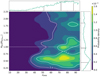 |
Fig. 10. Posterior probability density in the (σDRW, RBLR) parameter space marginalised over the microlensing parameters given ⟨M⟩ = 0.3 M⊙. RBLR is given in units of RBLRMK11 = 1.71 × 1017 cm, indicated by the white dashed line. The contours correspond to the 1 and 2−σ confidence intervals. Marginalised probability distributions of σDRW and RBLR are given in the top and right histograms respectively. In each histogram, the black line shows the 50th percentile (median value) of the distribution and the dashed lines highlight the 16th and 84th percentiles. Hence, we obtain |


5. Discussion
We now review the implications of the constraints on the accretion disk scale radius, R0, found using the three different models. The first model shows that the low-frequency variations of the microlensing light curve do not have a strong constraining power on R0 when using the power spectrum method. The second model indicates that the high-frequency part of the power spectrum adds significant constraints to the accretion disk measurement because the range of R0 compatible with the data is shrunk and leans towards the smallest values. Therefore, ignoring the high-frequency variations may lead to overestimation of R0.
The first two models, which rely only on microlensing variability, both require lower values of the mean stellar mass ⟨M⟩. However, a galaxy populated by stars with ⟨M⟩ = 0.01 M⊙ is barely conceivable because the least massive star known to this day has a mass of 0.07 M⊙ (Kasper et al. 2007). This means that, according to these two models, the population of compact objects that is most likely to produce the observed variability is not made of stars. Hypothetical populations of primordial black holes (Hawkins 2020b,a) and galaxies with a significant number of brown dwarfs and/or free-floating Jupiter-like planets (Dai & Guerras 2018; Cornachione et al. 2020a) have been invoked to explain unexpected microlensing features. Unfortunately, primordial black holes have, to date, never been observed in nearby galaxies despite huge efforts of multiple collaborations (Alcock et al. 2001; Niikura et al. 2019a,b). In addition, the theoretical mass of a primordial black hole is poorly constrained and spans the very broad range of [10−16,102] M⊙ (Green & Kavanagh 2020). Similarly, a low-mass stellar population is not observed in the Milky Way (Mróz et al. 2017). In both cases, the explanation behind the observed variability relies on an exotic population of microlenses in the lens galaxy for which we do not have any observational proof so far.
Continuum reverberation in the BLR is an acknowledged and observed effect (Blandford & McKee 1982; Bentz et al. 2009; Du et al. 2016; Williams et al. 2021) and supports the validity of our third model. The latter encapsulates our best understanding of microlensing light curve variability. It is also the only model that favours a more standard value of the mean stellar mass, ⟨M⟩ = 0.3 M⊙, which does not require any exotic population of microlenses. This suggests that reverberation of the continuum by the BLR, which was observed multiple times with spectroscopic monitoring, is also observable in single-band photometric light curves through their high-frequency variations on the differential light curve.
Last but not least, this offers a new way of measuring the size of the BLR illustrated by Fig. 10. The relative insensitivity of this measurement to the microlensing parameters (ve, R0) is due to the fact that, as stated in Sect. 4.1, the main challenge of a given set of parameters ζ is to fit the high-frequency power and these are mainly set by the reverberated variability. The downside of this is that we are not able to discriminate between the values of R0. Nevertheless, in the case of QJ 0158-4325, the measurement of RBLR is in agreement with the Hβ-BLR size–luminosity relation (Mosquera & Kochanek 2011).
6. Conclusions and perspectives
In this work, we present a new method whereby we use the power spectrum of microlensing light curves to study the strongly lensed quasar QJ 0158-4325 system. This method allows us to take into account the high-frequency variations of the data and simultaneously include the reverberated variability in the microlensing paradigm. Our main results are summed up in the following points:
-
Ignoring the high-frequency variations, as is the case with the light-curve-fitting method, may lead to an overestimation of the scale radius of the accretion disk R0. Indeed, we show that the use of short-timescale variations excludes the values of R0 found with the light-curve-fitting method in Morgan et al. (2012).
-
In the context of standard paradigm microlensing light-curve simulations, the data favour an exotic microlens population drawn from an IMF with an unprecedentedly low mean mass ⟨M⟩ whereas with the model we propose, including the BLR reverberation, the data favour stellar populations drawn from a standard Salpeter IMF with ⟨M⟩ = 0.3 M⊙.
-
For the first time, continuum reverberation by the BLR is observed in a single waveband photometric light curve. We use this opportunity to measure the size of the BLR in QJ 0158-4325, obtaining
 cm, which is compatible with the expectation of the luminosity–size relation with a better precision than standard photometric reverberation mapping techniques.
 -
The power-spectrum-fitting method is insensitive to the scale radius of the accretion disk R0 in the presence of reverberated variability in the single-waveband light curve.
In light of the encouraging results this method gave for QJ 0158-4325, we are looking forward to applying it to other systems for which a microlensing light curve is available. In the upcoming Vera C. Rubin Observatory era, this method offers a new way to probe the luminosity–BLR size relation of quasars for a large range of redshifts and luminosities.
The Event Horizon Telescope (https://eventhorizontelescope.org) can resolve the accretion disk while the BLR can be resolved using the VLT, although these are both limited to a handful of nearby AGNs.
Dai et al. (2010) show that accounting for a magnification offset due to contamination from the BLR of up to 40% translates into shrinkage of the measured accretion disk by up to 50%. However, these authors do not consider the impact of reverberation on the frequency content of the light curves.
Although Sluse et al. (2012) showed that 10%-20% of the flux is typically microlensed, Sluse & Tewes (2014) found that this effect marginally impacts the variations in the microlensing light curve.
Rin is very small compared to R0 and should not have an impact on the result because the half light radius R1/2 remains mostly unchanged.
The experiment ran with a uniform prior on the angle actually yields a 1−σ to 2−σ compatible measurement.
Acknowledgments
This work is supported by the Swiss National Science Foundation (SNSF) and by the European Research Council (ERC) under the European Union’s Horizon 2020 research and innovation program (COSMICLENS: grant agreement No 787886). G.V. has received funding from the European Union’s Horizon 2020 research and innovation program under the Marie Sklodovska-Curie grant agreement No 897124. The authors wish to thank Aymeric Galan for useful comments and graphical contribution. Finally, we thank the anonymous referee for the useful comments that improved the clarity of the paper.
References
- Alcock, C., Allsman, R. A., Alves, D. R., et al. 2001, ApJ, 550, L169 [NASA ADS] [CrossRef] [Google Scholar]
- Bate, N. F., Floyd, D. J. E., Webster, R. L., & Wyithe, J. S. B. 2008, MNRAS, 391, 1955 [NASA ADS] [CrossRef] [Google Scholar]
- Bate, N. F., Vernardos, G., O’Dowd, M. J., et al. 2018, MNRAS, 479, 4796 [NASA ADS] [CrossRef] [Google Scholar]
- Bentz, M. C., Walsh, J. L., Barth, A. J., et al. 2009, ApJ, 705, 199 [NASA ADS] [CrossRef] [Google Scholar]
- Blackburne, J. A., Pooley, D., & Rappaport, S. 2006, ApJ, 640, 569 [NASA ADS] [CrossRef] [Google Scholar]
- Blackburne, J. A., Pooley, D., Rappaport, S., & Schechter, P. L. 2011, ApJ, 729, 34 [Google Scholar]
- Blandford, R. D., & McKee, C. F. 1982, ApJ, 255, 419 [Google Scholar]
- Borguet, B., Hutsemékers, D., Letawe, G., Letawe, Y., & Magain, P. 2008, A&A, 478, 321 [NASA ADS] [CrossRef] [EDP Sciences] [Google Scholar]
- Cantale, N., Courbin, F., Tewes, M., Jablonka, P., & Meylan, G. 2016, A&A, 589, A81 [NASA ADS] [CrossRef] [EDP Sciences] [Google Scholar]
- Chan, J. H. H., Millon, M., Bonvin, V., & Courbin, F. 2020, A&A, 636, A52 [EDP Sciences] [Google Scholar]
- Chan, J. H. H., Rojas, K., Millon, M., et al. 2021, A&A, 647, A115 [NASA ADS] [CrossRef] [EDP Sciences] [Google Scholar]
- Chang, K., & Refsdal, S. 1979, Nature, 282, 561 [Google Scholar]
- Chen, B., Dai, X., Kochanek, C. S., et al. 2012, ApJ, 755, 24 [Google Scholar]
- Collin, S., Boisson, C., Mouchet, M., et al. 2002, A&A, 388, 771 [NASA ADS] [CrossRef] [EDP Sciences] [Google Scholar]
- Cornachione, M. A., & Morgan, C. W. 2020, ApJ, 895, 93 [Google Scholar]
- Cornachione, M. A., Morgan, C. W., Burger, H. R., et al. 2020a, ApJ, 905, 7 [NASA ADS] [CrossRef] [Google Scholar]
- Cornachione, M. A., Morgan, C. W., Millon, M., et al. 2020b, ApJ, 895, 125 [Google Scholar]
- Courbin, F., Eigenbrod, A., Vuissoz, C., Meylan, G., & Magain, P. 2005, in Gravitational Lensing Impact on Cosmology, ed. Y. Mellier, & G. Meylan, 225, 297 [NASA ADS] [Google Scholar]
- Czerny, B., & Hryniewicz, K. 2011, A&A, 525, L8 [NASA ADS] [CrossRef] [EDP Sciences] [Google Scholar]
- Dai, X., & Guerras, E. 2018, ApJ, 853, L27 [NASA ADS] [CrossRef] [Google Scholar]
- Dai, X., Kochanek, C. S., Chartas, G., et al. 2010, ApJ, 709, 278 [Google Scholar]
- Ding, X., Liao, K., Treu, T., et al. 2017a, MNRAS, 465, 4634 [NASA ADS] [CrossRef] [Google Scholar]
- Ding, X., Treu, T., Suyu, S. H., et al. 2017b, MNRAS, 472, 90 [NASA ADS] [CrossRef] [Google Scholar]
- Ding, X., Treu, T., Birrer, S., et al. 2021, MNRAS, 501, 269 [Google Scholar]
- Du, P., Lu, K.-X., Hu, C., et al. 2016, ApJ, 820, 27 [NASA ADS] [CrossRef] [Google Scholar]
- Edelson, R., Gelbord, J. M., Horne, K., et al. 2015, ApJ, 806, 129 [NASA ADS] [CrossRef] [Google Scholar]
- Eigenbrod, A., Courbin, F., Vuissoz, C., et al. 2005, A&A, 436, 25 [NASA ADS] [CrossRef] [EDP Sciences] [Google Scholar]
- Eigenbrod, A., Courbin, F., Meylan, G., et al. 2008a, A&A, 490, 933 [NASA ADS] [CrossRef] [EDP Sciences] [Google Scholar]
- Eigenbrod, A., Courbin, F., Sluse, D., Meylan, G., & Agol, E. 2008b, A&A, 480, 647 [NASA ADS] [CrossRef] [EDP Sciences] [Google Scholar]
- Elvis, M. 2000, ApJ, 545, 63 [NASA ADS] [CrossRef] [Google Scholar]
- Faure, C., Anguita, T., Eigenbrod, A., et al. 2009, A&A, 496, 361 [NASA ADS] [CrossRef] [EDP Sciences] [Google Scholar]
- Floyd, D. J. E., Bate, N. F., & Webster, R. L. 2009, MNRAS, 398, 233 [NASA ADS] [CrossRef] [Google Scholar]
- Gebhardt, K., Bender, R., Bower, G., et al. 2000, ApJ, 539, L13 [Google Scholar]
- Green, A. M., & Kavanagh, B. J. 2020, Primordial Black Holes as a dark matter candidate [Google Scholar]
- Grier, C. J., Shen, Y., Horne, K., et al. 2019, ApJ, 887, 38 [NASA ADS] [CrossRef] [Google Scholar]
- Harris, F. J. 1978, Proc. IEEE, 66, 51 [NASA ADS] [CrossRef] [Google Scholar]
- Hawkins, M. R. S. 2020a, A&A, 643, A10 [NASA ADS] [CrossRef] [EDP Sciences] [Google Scholar]
- Hawkins, M. R. S. 2020b, A&A, 633, A107 [NASA ADS] [CrossRef] [EDP Sciences] [Google Scholar]
- Homayouni, Y., Trump, J. R., Grier, C. J., et al. 2019, ApJ, 880, 126 [NASA ADS] [CrossRef] [Google Scholar]
- Hu, C., Du, P., Lu, K.-X., et al. 2015, ApJ, 804, 138 [Google Scholar]
- Ivezić, V., & MacLeod, C. 2013, Proc. Int. Astron. Union, 9, 395 [CrossRef] [Google Scholar]
- Karouzos, M., Woo, J.-H., Matsuoka, K., et al. 2015, ApJ, 815, 128 [NASA ADS] [CrossRef] [Google Scholar]
- Kasper, M., Biller, B. A., Burrows, A., et al. 2007, A&A, 471, 655 [NASA ADS] [CrossRef] [EDP Sciences] [Google Scholar]
- Kaspi, S., Brandt, W. N., Maoz, D., et al. 2021, ApJ, submitted [arXiv:2106.00691] [Google Scholar]
- Kelly, B. C., & Siemiginowska, A. 2009, ApJ, 698, 895 [NASA ADS] [CrossRef] [Google Scholar]
- Khadka, N., Yu, Z., Zajaček, M., et al. 2021, MNRAS, 508, 4722 [NASA ADS] [CrossRef] [Google Scholar]
- Kochanek, C. S. 2004, ApJ, 605, 58 [Google Scholar]
- Kogut, A., Lineweaver, C., Smoot, G. F., et al. 1993, ApJ, 419, 1 [NASA ADS] [CrossRef] [Google Scholar]
- Krolik, J. H., Horne, K., Kallman, T. R., et al. 1991, ApJ, 371, 541 [Google Scholar]
- Li, S.-S., Yang, S., Yang, Z.-X. 2021, ApJ, 920, 9 [NASA ADS] [CrossRef] [Google Scholar]
- Lobban, A. P., Zola, S., Pajdosz-Śmierciak, U., et al. 2020, MNRAS, 494, 1165 [NASA ADS] [CrossRef] [Google Scholar]
- MacLeod, C. L., Ivezić, Ž., Kochanek, C. S., et al. 2010, ApJ, 721, 1014 [Google Scholar]
- MacLeod, C. L., Ross, N. P., Lawrence, A., et al. 2016, MNRAS, 457, 389 [Google Scholar]
- Magain, P., Courbin, F., & Sohy, S. 1998, ApJ, 494, 472 [NASA ADS] [CrossRef] [Google Scholar]
- Mediavilla, E., Muñoz, J., Kochanek, C., et al. 2011, ApJ, 730, 16 [NASA ADS] [CrossRef] [Google Scholar]
- Millon, M., Courbin, F., Bonvin, V., et al. 2020a, A&A, 642, A193 [NASA ADS] [CrossRef] [EDP Sciences] [Google Scholar]
- Millon, M., Courbin, F., Bonvin, V., et al. 2020b, A&A, 640, A105 [NASA ADS] [CrossRef] [EDP Sciences] [Google Scholar]
- Millon, M., Tewes, M., Bonvin, V., Lengen, B., & Courbin, F. 2020c, J. Open Source Softw., 5, 2654 [NASA ADS] [CrossRef] [Google Scholar]
- Morgan, N. D., Dressler, A., Maza, J., Schechter, P. L., & Winn, J. N. 1999, AJ, 118, 1444 [NASA ADS] [CrossRef] [Google Scholar]
- Morgan, C. W., Eyler, M. E., Kochanek, C., et al. 2008, ApJ, 676, 80 [NASA ADS] [CrossRef] [Google Scholar]
- Morgan, C. W., Kochanek, C., Morgan, N. D., & Falco, E. E. 2010, ApJ, 712, 1129 [NASA ADS] [CrossRef] [Google Scholar]
- Morgan, C. W., Hainline, L. J., Chen, B., et al. 2012, ApJ, 756, 52 [Google Scholar]
- Morgan, C. W., Hyer, G. E., Bonvin, V., et al. 2018, ApJ, 869, 106 [Google Scholar]
- Mortonson, M. J., Schechter, P. L., & Wambsganss, J. 2005, ApJ, 628, 594 [NASA ADS] [CrossRef] [Google Scholar]
- Mosquera, A. M., & Kochanek, C. S. 2011, ApJ, 738, 96 [Google Scholar]
- Motta, V., Mediavilla, E., Rojas, K., et al. 2017, ApJ, 835, 132 [NASA ADS] [CrossRef] [Google Scholar]
- Mróz, P., Udalski, A., Skowron, J., et al. 2017, Nature, 548, 183 [Google Scholar]
- Mudd, D., Martini, P., Zu, Y., et al. 2018, ApJ, 862, 123 [Google Scholar]
- Neira, F., Anguita, T., & Vernardos, G. 2020, MNRAS, 495, 544 [NASA ADS] [CrossRef] [Google Scholar]
- Niikura, H., Takada, M., Yasuda, N., et al. 2019a, Nat. Astron., 3, 524 [NASA ADS] [CrossRef] [Google Scholar]
- Niikura, H., Takada, M., Yokoyama, S., Sumi, T., & Masaki, S. 2019b, Phys. Rev. D, 99 [CrossRef] [Google Scholar]
- Peng, C. Y., Impey, C. D., Rix, H.-W., et al. 2006, ApJ, 649, 616 [Google Scholar]
- Penton, A., Malik, U., Davis, T., et al. 2022, MNRAS, 509, 4008 [Google Scholar]
- Peterson, B. 2006, in The Broad-Line Region in Active Galactic Nuclei, eds. D. Alloin, R. Johnson, & P. Lira (Berlin, Heidelberg: Springer, Berlin Heidelberg), 77 [Google Scholar]
- Peterson, B. M., Ali, B., Horne, K., et al. 1993, ApJ, 402, 469 [NASA ADS] [CrossRef] [Google Scholar]
- Poindexter, S., & Kochanek, C. S. 2010, ApJ, 712, 668 [NASA ADS] [CrossRef] [Google Scholar]
- Refsdal, S. 1964, MNRAS, 128, 307 [NASA ADS] [CrossRef] [Google Scholar]
- Rojas, K., Motta, V., Mediavilla, E., et al. 2014, ApJ, 797, 61 [Google Scholar]
- Rojas, K., Motta, V., Mediavilla, E., et al. 2020, ApJ, 890, 3 [Google Scholar]
- Schmidt, R. W., & Wambsganss, J. 2010, Gen. Relativ. Gravit., 42, 2127 [Google Scholar]
- Shakura, N. I., & Sunyaev, R. A. 1973, A&A, 24, 337 [NASA ADS] [Google Scholar]
- Sluse, D., & Tewes, M. 2014, A&A, 571, A60 [NASA ADS] [CrossRef] [EDP Sciences] [Google Scholar]
- Sluse, D., Claeskens, J. F., Hutsemékers, D., & Surdej, J. 2007, A&A, 468, 885 [NASA ADS] [CrossRef] [EDP Sciences] [Google Scholar]
- Sluse, D., Hutsemékers, D., Courbin, F., Meylan, G., & Wambsganss, J. 2012, A&A, 544, A62 [NASA ADS] [CrossRef] [EDP Sciences] [Google Scholar]
- Suberlak, K. L., Ivezić, Ž., & MacLeod, C. 2021, ApJ, 907, 96 [NASA ADS] [CrossRef] [Google Scholar]
- Tewes, M., Courbin, F., & Meylan, G. 2013, A&A, 553, A120 [NASA ADS] [CrossRef] [EDP Sciences] [Google Scholar]
- Tremblay, G. R., Oonk, J. B. R., Combes, F., et al. 2016, Nature, 534, 218 [NASA ADS] [CrossRef] [Google Scholar]
- Urry, C. M., & Padovani, P. 1995, PASP, 107, 803 [NASA ADS] [CrossRef] [Google Scholar]
- Vernardos, G., & Fluke, C. J. 2014, MNRAS, 445, 1223 [NASA ADS] [CrossRef] [Google Scholar]
- Vernardos, G., & Tsagkatakis, G. 2019, MNRAS, 486, 1944 [NASA ADS] [CrossRef] [Google Scholar]
- Vernardos, G., Fluke, C. J., Bate, N. F., Croton, D., & Vohl, D. 2015, ApJS, 217, 23 [CrossRef] [Google Scholar]
- Williams, P. R., Treu, T., Dahle, H., et al. 2021, ApJ, 911, 64 [NASA ADS] [CrossRef] [Google Scholar]
- Wong, K. C., Suyu, S. H., Auger, M. W., et al. 2017, MNRAS, 465, 4895 [NASA ADS] [CrossRef] [Google Scholar]
- Wong, K. C., Suyu, S. H., Chen, G. C. F., et al. 2020, MNRAS, 498, 1420 [Google Scholar]
- Yu, Z., Martini, P., Davis, T. M., et al. 2020, ApJS, 246, 16 [Google Scholar]
- Zhang, Z.-X., Du, P., Smith, P. S., et al. 2019, ApJ, 876, 49 [NASA ADS] [CrossRef] [Google Scholar]
- Zu, Y., Kochanek, C. S., & Peterson, B. M. 2011, ApJ, 735, 80 [NASA ADS] [CrossRef] [Google Scholar]
- Zu, Y., Kochanek, C. S., Kozłowski, S., & Udalski, A. 2013, ApJ, 765, 106 [NASA ADS] [CrossRef] [Google Scholar]
All Tables
All Figures
|
Fig. 1. Schematic view of the relative location and size of the different regions of a quasar and illustration of the reverberation effect. RS is the Schwarzschild radius of the central SMBH. The continuum light from the central accretion disk (red) is reverberated both in the BLR (green) and in the NLR (blue), which are much larger than the accretion disk and are therefore much less affected by microlensing (see Sect. 3.3). |
| In the text | |
|
Fig. 2. QJ 0158-4325 observed with the Hubble Space Telescope in the F814W filter (program ID 9267; PI: Beckwith). The microlensing magnification maps (corresponding to ⟨M⟩ = 0.3 M⊙) are shown for each quasar image using the same colour scale, and are rotated with respect to the shear angle. The green line indicates a realisation of a trajectory of the source, the same in orientation and length for both maps drawn from the probability density function of ve shown on Fig. 5. |
| In the text | |
|
Fig. 3. Top: COSMOGRAIL R-band light curves of images A and B of QJ 0158-4325 over a period of 13 years. For clarity, the B curve has been artificially shifted upwards by 0.2 mag (adapted from Millon et al. 2020b). Middle: microlensing light curve (red) obtained from the observations using Eq. (2) with ΔtAB = 22.7 days (Millon et al. 2020b), along with examples of spline fitting with different values of the η parameter (defined in Sect. 2.2). Bottom: residuals of the three illustrative spline fits to the microlensing light curve. The number on the left indicates the artificial shifts applied for the purpose of clarity. |
| In the text | |
|
Fig. 4. Power spectrum of the observed microlensing light curve computed as the mean of the power spectra obtained for 1000 different realisations of photometric noise for every value of η sampling the range [30:100] days with steps of 5 days used for the spline fitting parameter (see text). The 1−σ envelope is given by the standard deviation of the same set of power spectra. The dashed black line marks the boundary between low and high frequency and the grey area indicates our adopted frequency limit of 10−2 days−1, below which photometric uncertainties dominate the data. |
| In the text | |
|
Fig. 5. Probability density of the effective velocity, ve, in the source plane for QJ 0158-4325 from Eq. (11). |
| In the text | |
|
Fig. 6. Top panel: example of a simulated light curve with and without reverberation (dotted and solid lines respectively). Bottom panel: corresponding power spectra. The curves and power spectra have been produced using ⟨M⟩ = 0.3 M⊙, ve = 1236 km s−1, R0 = 0.5RMK11, σDRW = 30 and RBLR = RBLRMK11. Adding reverberation clearly adds power to the high-frequency part of the spectrum. |
| In the text | |
|
Fig. 7. Mean (lines) and upper 1−σ envelope (shaded area) of power spectra from 100 000 simulated curves for different (ve, R0) configurations, in the absence of reverberation (FBLR = 0 in Eq. (3)), compared to the data (same as Fig. 4). Due to the logarithmic scale, the lower envelopes extend almost to the x-axis and are not displayed for clarity. The vertical dashed line marks the boundary between low and high frequency. |
| In the text | |
|
Fig. 8. Slices of the marginalised posterior probability of the (ve, R0, ⟨M⟩) parameter space (three-dimensional after the marginalisation over the angle of ve using Eq. (17)) for each of the three models described in Sect. 4. Model LF: light curves simulated without reverberation and fitted only to the low-frequency data, i.e. up to 1/750 days−1, which corresponds to the same frequency cut as in Morgan et al. (2012). Model FF: same simulations are fitted to the full frequency range, i.e. up to 1/100 days−1. Model RFF: light curves are now simulated with reverberation (fBLR = 0.432 ± 0.036, σDRW = 55 and RBLR = RBLRMK11) and the full observed frequency range up to 1/100 days−1 is considered. The solid line corresponds to RMK11, the estimate of Mosquera & Kochanek (2011), the ellipse represents the (ve, R0) measurement interval from Morgan et al. (2012). The coloured contours encapsulate [10–100]% of the probability volume and are projected in each of the displayed slices. We note that our probability densities are not scaled by the evidence and therefore cannot be compared across different models. |
| In the text | |
|
Fig. 9. Effect of the reverberation process on the power spectrum. The data are shown as a solid red line. The coloured envelopes display the power spectra from 100 000 simulated curves for different values of RBLR. Each panel considers different values for σDRW. In this plot we use R0 = RMK11, ⟨M⟩ = 0.3 M⊙, ve = 700 km s−1, and fBLR = 0.432 ± 0.036. The black dashed line marks the boundary between low and high frequency. While the high-frequency range is never well represented with pure microlensing (blue), it is very sensitive to a change in the reverberation parameters. |
| In the text | |
|
Fig. 10. Posterior probability density in the (σDRW, RBLR) parameter space marginalised over the microlensing parameters given ⟨M⟩ = 0.3 M⊙. RBLR is given in units of RBLRMK11 = 1.71 × 1017 cm, indicated by the white dashed line. The contours correspond to the 1 and 2−σ confidence intervals. Marginalised probability distributions of σDRW and RBLR are given in the top and right histograms respectively. In each histogram, the black line shows the 50th percentile (median value) of the distribution and the dashed lines highlight the 16th and 84th percentiles. Hence, we obtain |
| In the text | |
Current usage metrics show cumulative count of Article Views (full-text article views including HTML views, PDF and ePub downloads, according to the available data) and Abstracts Views on Vision4Press platform.
Data correspond to usage on the plateform after 2015. The current usage metrics is available 48-96 hours after online publication and is updated daily on week days.
Initial download of the metrics may take a while.