| Issue |
A&A
Volume 658, February 2022
|
|
|---|---|---|
| Article Number | A107 | |
| Number of page(s) | 11 | |
| Section | Planets and planetary systems | |
| DOI | https://doi.org/10.1051/0004-6361/202142110 | |
| Published online | 09 February 2022 | |
The similarity of multi-planet systems
1
Observatoire Astronomique de l’Université de Genève,
51 Ch. des Maillettes,
Sauverny,
1290
Versoix, Switzerland
e-mail: This email address is being protected from spambots. You need JavaScript enabled to view it.
2
Institute for Computational Science, University of Zurich,
Winterthurerstr. 190,
8057
Zurich, Switzerland
Received:
30
August
2021
Accepted:
6
December
2021
Abstract
Previous studies using Kepler data suggest that planets orbiting the same star tend to have similar sizes. However, due to the faintness of the stars, only a few of the planets were also detected with radial velocity follow-ups, and therefore the planetary masses were mostly unknown. It is therefore yet to be determined whether planetary systems indeed behave like “peas in a pod”. Follow-up programs of TESS targets significantly increased the number of confirmed planets with mass measurements, allowing for a more detailed statistical analysis of multi-planet systems. In this work we explore the similarity in radii, masses, densities, and period ratios of planets within planetary systems. We show that planets in the same system that are similar in radii could be rather different in mass and vice versa, and that typically the planetary radii of a given planetary system are more similar than the masses. We also find a transition in the peas in a pod pattern for planets more massive than ~100 M⊕ and larger than ~10 R⊕. Planets below these limits are found to be significantly more uniform. We conclude that other quantities, such as density, may be crucial to fully understanding the nature of planetary systems and that, due to the diversity of planets within a planetary system, increasing the number of detected systems is crucial for understanding the exoplanetary demographics.
Key words: planets and satellites: general / planets and satellites: detection
© ESO 2022
1 Introduction
The number of discovered exoplanets has increased to over 4000 thanks to various ground-based and space-based surveys, among which NASA’s Kepler mission (Borucki et al. 2010) stands out with more than 2300 discovered planets. This large sample of exoplanets has allowed the detailed statistical analyses of hundreds of multi-planetary systems (e.g., Lissauer et al. 2011, 2012, 2014; Latham et al. 2011; Rowe et al. 2014), which have expanded our knowledge on aspects such as physical composition (e.g., Carter et al. 2012; Hadden & Lithwick 2014) and orbital eccentricity and inclination (e.g., Fang & Margot 2012; Fabrycky et al. 2014; Xie et al. 2016; Van Eylen et al. 2019). Although these properties in multi-planetary systems have triggered multiple studies of their formation and evolution histories (e.g., Hansen & Murray 2013; Steffen & Hwang 2015; Malhotra 2015; Ballard & Johnson 2016; Mills et al. 2016; Owen & Campos Estrada 2020), our understanding of the diversity of planetary systems is still incomplete.
It was suggested by Weiss et al. (2018) that planetary systems are like “peas in a pod” (i.e., multi-transiting systems tend to have planets with similar sizes and to be regularly spaced). Weiss et al. (2018) used a large sample of Kepler multi-planetary systems whose parameters were refined by the California-Kepler Survey (CKS Petigura et al. 2017), and employed a series of bootstrap tests to quantify the significance of the similarity between sizes; they concluded that the observed distribution could not be explained by random resampling. While Zhu (2020) argued that the result by Weiss et al. (2018) is affected by observational biases, a strong evidence that the observed intra-system uniformity has an astrophysical origin has been confirmed by other studies (e.g., Weiss & Petigura 2020; Murchikova & Tremaine 2020; Gilbert & Fabrycky 2020; Jiang et al. 2020; Mishra et al. 2021). A similar statistical approach was presented by Millholland et al. (2017), who used a sample of planets with masses characterized by transit timing variations (TTVs) from Hadden & Lithwick (2017) and found that planets orbiting the same star also tend to have similar masses. The similarity in mass was based on a rather restricted sample of planetary systems. They analyzed a sample of 37 systems with masses below 50 M⊕ derived by the TTV. Due to the faintness of the stars targeted by Kepler, only a small fraction of the detected planets were suitable for radial velocity (RV) follow-up.
After the end of the primary Kepler mission, NASA’s K2 mission continued to discover transiting planets orbiting stars near the ecliptic plane (Howell et al. 2014). Compared to Kepler, the K2 mission covered more sky, observed more diverse stellar populations, and focused on brighter targets, which are more suitable for RV follow-up observations. Later, the Transiting Exoplanet Survey Satellite (TESS) was launched in 2018 to survey 85% of the sky for transiting exoplanets around bright stars (Ricker et al. 2015). RV follow-up programs have triggered a rapid expansion of the number of confirmed planets with a mass measurement, which has allowed an in-depth analysis of the peas in a pod pattern to be performed in terms of mass with a larger and a more diverse sample of planetary systems.
In this paper we revisit the details of several aspects of the peas in a pod pattern (i.e., the radius, mass, and period ratio correlation) by accounting for observational biases and using different exoplanet catalogs. The paper is organized as follows. In Sect. 2 we analyze the uniformity of planetary systems in mass and radius. In Sect. 3 we study the uniformity in the period spacing. Our conclusions are summarized in Sect. 4.
2 Similarity in mass, radius and density
2.1 Exoplanet sample
We used the NASA Exoplanet Archive1 (Akeson et al. 2013) on August 2021 since it is the most up-to-date catalog. We excluded the less accurate data by considering only planets with measurement uncertainties smaller than σM ∕M = 50% and σR ∕R = 16%, which leaves us with 144 planets that are part of 48 multi-planet systems. We note that the limits on the mass and radius uncertainties of the planets in the present sample are twice the values used in Otegi et al. (2020), where we presented an updated exoplanet catalog based on reliable mass and radius measurements of transiting planets with uncertainties smaller than σM ∕M = 25% and σR ∕R = 8%. In Otegi et al. (2020) our aim was to build a catalog with as accurate mass and radius measurements as possible in order to derive a mass–radiusrelationship, while in this work we prefer to relax the limits in order to include more multi-planet systems. More specifically, the catalog presented in Otegi et al. (2020) contains 23 multi-planet systems, which is half of the sample used here. The impact of the choice of the limits on the uncertainties on mass and radius is discussed in Sect. 2.7. Twenty-seven of the systems in our sample were characterized via TTVs, and 21 by RVs. Of the 37 systems used in Millholland et al. (2017), 16 are included in our catalog while 21 systems were discarded due to large uncertainties or for not being considered “robust” in Hadden & Lithwick (2017). Among the RVs, only one system in our catalog (HD 219134) is also present in the study by Wang (2017), since the rest of their systems are composed of non-transiting planets.
Clearly, the results depend on the available data and could be affected by selection biases from the radial velocity, transit timing variations, or transit methods. This effect can be reduced using homogeneous samples of planets with well-determined selection biases. This was done by Weiss et al. (2018) and Millholland et al. (2017), who used only Kepler planets and planets characterized by TTVs, respectively. However, for this work our aim was to have a large and diverse sample, which results in a less homogeneous sample.
2.2 Similarity metric
Several approaches have been taken to analyze the architectures of planetary systems. For example, Kipping (2018) proposed a model to define the entropy of a planetary system’s size-ordering; Gilbert & Fabrycky (2020) suggested different descriptive measures to characterize the arrangements of planetary masses, periods, and mutual inclinations. Alibert (2019) defined a new metric to infer the similarity between two planetary systems that was based on representing the planets of the systems as points on a logarithmic radius-period plane, and spreading the points with a Gaussian kernel whose weights correspond to the planet masses. A similar approach without using a Gaussian kernel estimation of the probability distribution was used by Bashi & Zucker (2021). In this work we use an approach, similar to the one used in Millholland et al. (2017), where we quantify the similarity of the systems by considering the distance in the logarithmic space, which can be expressed as
 (1)
(1)
with an equivalent expression for  . The value of
 is computedby summing the distances in logarithmic space of adjacent planets, normalized by the number of pairs Np -1 in order to remove the dependency on the number of planets in the system. We note that for this metric lower values correspond to more similarity. We can also consider the global distance in the log Mp -log Rp space as an indicator of the similarity of a planetary system. Similarly to the expression for
  , the global distance can be given by
![Mathematical equation: \begin{equation*} \mathcal{D}= \sum ^{N_{\textrm{pl}}-1} _{\substack{i=1\\ P_i<P_{i+1}}} \bigg[ \ \bigg(\textrm{log} \frac{M_{i+1}}{M_{i}} \bigg){}^2 + \bigg(\textrm{log} \frac{R_{i+1}}{R_{i}} \bigg){}^2 \ \bigg] ^{1/2} \ \bigg/ \ N_{\textrm{pl}}-1. \end{equation*}](/articles/aa/full_html/2022/02/aa42110-21/aa42110-21-eq5.png) (2)
(2)
Table A.1 lists the radius, mass, and global similarities of all the systems in our sample based on this metric. We also list the results for the planets in the Solar System, and for the inner and outer parts of it. In order to ensure that our results do not strongly depend on the metric, we compare the results using the variance in log-space of mass and radius and find that the inferred ranking is nearly identical. Kepler 60 is found to be the most uniform system; it includes three rocky planets below the radius valley. The next four similar uniform systems include pairs of rocky exoplanets (L 98-56) or sub-Neptunes (Kepler 29, TOI 763, Kepler 26). The less uniform systems are Kepler 87, WASP 47, Kepler 289, Kepler 30, and Kepler 117. However, we suspect that not all the planets in the systems have been detected. The inherent detection limits of the radial velocity, transit timing variation, and transit methods do not give a full picture of the orbital architecture. For each system we may be missing relatively small planets, or planets at large orbital distances. The detection of these missing planets would increase the metric  , making them less similar. The lack of the missing planets may explain the result that the Solar System is the fifth least similar system. Interestingly, even when we consider only the inner Solar System, or only the outer Solar System, it is always found to be the least similar planetary system. The weak similarity of the outer Solar System is explained by the difference between Uranus and Neptune with the gas giants, while the weak similarity of the terrestrial planets is mainly due to Mercury.
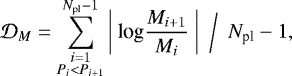
Figure 1 shows the orbital architecture of the multi-planet systems in our sample. The color of the points represent log  (left panel) and log
  (right panel), and the planets are ordered by the similarity in
  (left panel) and by the similarity in
  (right panel).
Before making a proper quantitative analysis, there are a few architectural features that appear in Fig. 1. First, we see that planetary systems in our sample tend to be more similar in radius than in mass. Figure 2 shows the histogram of  and
and  (the full list of the values can be seen in Table A.1), showing that the values of
  are much lower than those of
  . We clearly see that there are significantly more systems with
  < 0.25 (35 systems) than with
  < 0.25 (25 systems). This is not caused by the larger range in planetary masses than in planetary radii since the metric we use is insensitive to the size of the range. This could be explained if the density tends to be similar in a planetary system. Since the density is three times more sensitive to radius variations than to mass variations, it is expected to have a stronger uniformity in radius than in mass. More specifically, in this case we would expect the systems to be three times less similar in mass than in radius. We find that the median of
  is 1.75 times larger than that of
  . Figure 3 shows
  plottted against
  , with a line corresponding to
  = 3
= 3  . It is interesting to note that the
  = 3
= 3  line does not fit the observed population. However, as we discuss below, this could be a result of the uniformity in density. The uniformity in density within a planetary system is further discussed in Sect. 2.4. We also find that the distribution of
  extends to higher values. The tail seen in the
  distribution corresponds to five particular systems that include a giant planet and a sub-Neptune.
Second, we find that generally the planets that are most similar in radius are not the ones that are most similar in mass, as illustrated in Fig. 3. Even if there is a weak correlation between the similarities in mass and radii, the dispersion is very large, especially among the most similar systems. It should also be noted that there is a clear dependence on stellar mass: low-mass stars are more concentrated in the lower part of Fig. 3, indicating that planets orbiting low-mass stars tend to be more similar in radius than in mass. In addition, M dwarfs closely follow the  = 3
= 3  relation. Since low-mass stars tend to host low-mass planets (Lozovsky et al. 2021), this behavior might hint that the physical processes during planet formation tend to produce planets of similar density in planetary systems around low-mass stars, leading to a similarity in radius that is three times stronger than in mass. The correlations with the host star mass are further discussed in Sect. 2.6.
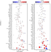 |
Fig. 1 Orbital architectures of the 48 multi-planet systems in our sample with measurement uncertainties smaller than σM ∕M = 50% and σR ∕R = 16%, and that of the inner Solar System. In the left panel the colors of the points represent the logarithm of the radius of a planet divided by the radius of the previous one, and the systems are ordered by similarity in radius (defined in Sect. 2.2). In the right panel the same is represented, but for the mass. The circle size is proportional to the radius of the planet. |
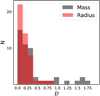 |
Fig. 2 Histograms of the distances |


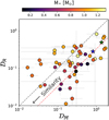 |
Fig. 3 Similarity in radius |


2.3 Correlation of mass and radius
Figure 4 shows the mass and radius of a planet against the mass and radius of the next planet. First we note that most of the pairs are above the 1:1 line, especially for the radius. This indicates that larger planets are found at larger orbital periods, which is in agreement with the findings in several other papers (e.g., Ciardi et al. 2013; Millholland et al. 2017; Kipping 2018; Weiss et al. 2018). Even if at long periods it is easier to detect larger and/or more massive planets, Helled et al. (2016) showed that the observed correlation between planetary radius and orbital period remains even after removing the effect of observational biases, and therefore it is unlikely to be caused solely by observational biases. Using the Pearson correlation test we find that there is a clear correlation for both mass and radius with P-values of 6 × 10⁻⁴ and 10−9, respectively (we note that the calculation of the Pearson coefficients do not include the uncertainties in mass and radius).This indicates that adjacent planets in a multi-planet system are likely to have similar masses and radii. We note that the P-value is significantly smaller for the planetary radii, suggesting that the peas in a pod pattern is less strong when it comes to the planetary mass. This is also clear from Fig. 1, where the color of the dots is more intense in the panel corresponding to the mass than in the panel corresponding to the radius.
It is also interesting to note that there is a clear transition in the uniformity of systems in both mass and radius plots. Figure 4 also shows a transition in the uniformity of planets around 25–100 M⊕ and 5–10 R⊕ (i.e., systems below these limits tend to be very uniform, and above are not correlated). We then study how the peas in a pod pattern depends on the mass range covered by the exoplanet sample. Figure 5 shows the dependence of the P-value on the mass and radius limits applied to the planetary sample. We find that removing the systems containing pairs of planets with masses higher than 100 M⊕ leads to a much stronger correlation. When we impose limits for the mass below 100 M⊕ the P-value increases. However, since samples with fewer points have higher P-values, this could be partly explained by the smaller number of pairs in the sample. We therefore explore the impact of the number of pairs when computing the P-value and the R-value. To do so, we randomly remove pairs from the initial sample, and compute the P-value and R-value. We repeated this process 1000 times; the median of the distribution and the 1σ error are shown in Fig. A.2. We find that randomly removing pairs leads to a rapid increase in the P-value. When changing the upper mass limit of 100 M⊕ to an upper mass limit of 15 M⊕, the number of pairs changes from 58 to 46 and the P-value from 4 × 10⁻¹⁰ to 3 × 10⁻⁴. However, when we randomly removed 12 pairs from an initial sample of 58 we expected a P-value between 3 × 10⁻⁸ and 2 × 10⁻⁶. Consequently, the increase in the P-values when lowering the mass limit to planets below 100 M⊕ cannot be completely explained by the decrease in number of points. We therefore identify a change in tendency in mass at 100 M⊕. This result agrees with the analysis performed by Wang (2017) using a sample of 27 non-transiting multi-planetary systems derived by RVs with minimum masses only.
We repeated the same analysis with the radius, and investigate the dependency of the P-value and the R-value on the radius limit applied to the planetary sample. We find that the results are nearly identical to the values inferred when applying limits on the mass range because the excluded planets are mostly the same. We find that when we exclude giant planets with radii larger than 10 R⊕ the peas in a pod pattern becomes more significant, but when imposing lower values to the upper limit of the radius there is an increase in the P-value that cannot be explained solely by the smaller number of pairs. We conclude that the change in tendency occurs at a radius of ~10 R⊕. We note that both transition points in mass and radius correspond to Saturn-like planets. It is clear that planetary systems tend to consist of planets with similar masses and radii, except for planets more massive or larger than Saturn. Even if current data indicate a minimum of the P-value at around ~100 M⊕ and ~10 R⊕, the precise location of these transitions should be analyzed in detail in future studies.
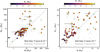 |
Fig. 4 Mass (left) or radius (right) of a planet against the mass or radius of the next planet (farther from the star). The color of the dots represents the mass of the host star. The green stars correspond to the Solar System planets and the gray points to a bootstrap trial. |
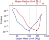 |
Fig. 5 P-value against the upper mass limit (blue) and upper radius limit (red) of the exoplanet sample. The dashed lines indicate the mass and radius at the minimum. |
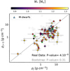 |
Fig. 6 Planetary density against the densities of the next planet farther from the star. The colors of the dots represent the effective temperature of the host star, and the gray dots correspond to a bootstrap trial. Pairs of planets orbiting around M dwarfs are represented by light blue triangles. The planets in the Solar System are indicated by the green stars. |
2.4 Density correlation
We find that planetary systems tend to be more similar in radius than in mass. It is therefore interesting to investigate the similarity in planetary density. If the density tends to be uniform within a planetary system, systems would be more similar in radius than in mass simply because of the stronger dependence of the density on the radius. Figure 6 shows the density of the planets in our sample against the densities of the next farthest planet from the star. We find a very strong correlation between the densities of adjacent planets (with a P-value of 4 × 10⁻⁹), and we do not find a clear and obvious bi-modality behavior like those observed in Fig. 4 for mass and radius. Interestingly, we also find that despite the small number of pairs of planets orbiting around M dwarfs, they tend to be close the 1:1 line in comparison to pairs around FGK stars. However, this trend is obtained from a sample of seven pairs; it needs to be confirmed when more data become available.
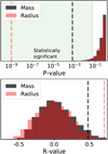 |
Fig. 7 Calculated P-value (top) and R-value (bottom) corresponding to the correlation between the mass (black) or radius (red) of a planet and the mass or radius of the next farthest planet. The dashed lines correspond to the results from the exoplanet sample and the histograms to the results of 3000 bootstrap trials. The green region in the upper panel shows the statistically significant region, where the P-value is smaller than 0.05. |
2.5 Significance and biases
Even when the correlation between radii, masses, and densities of adjacent planets is clear, it remains unknown whether thecorrelation is physical or is a consequence of observational biases. In order to investigate the role of detection biases, we perform a series of null hypothesis bootstrap tests. If detection biases are responsible for the observed correlation, then this trend would also be present in a mock exoplanetary population that does not have this trend inherently, but suffers from the same detection biases. The null hypothesis used in the bootstrap tests is that the size and mass of a planet is random and independent of the size and mass of its neighbor. We then subject the resulting sample to the detection biases, and investigate whether a correlation arises. We construct the bootstrap trial drawing random planetary masses from the distribution of the observed masses. Then, to each stellar host we assign a number of planetary masses equal to the number of planets detected and place them at the observed orbital periods. As discussed in Steffen (2016), the sensitivity of TTVs and RVs can be expressed by
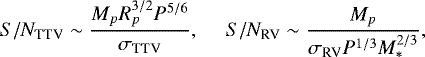 (3)
(3)
where σ is the intrinsic uncertainty of a measurement. In order to consider the detection efficiency on the transit we use the following expression for the S/N:
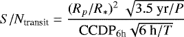 (4)
(4)
with
 (5)
(5)
Here Rp and R* are the sizes of the planet and the host star, respectively, P the orbital period, ρ* the bulk density of the star, and CCDP6h the six-hour combined differential photometric precision (the root mean square of the stellar photometric noise over six hours; Christiansen et al. 2012). We then follow a method similar to that used in Weiss & Petigura (2020): we randomly draw planets from a log-normal distribution until its S/N is high enough to be detected. We set a limit for S/NRV and S/NTTV of 2, and assume an intrinsic RV uncertainty of 2 m s−1. These S/N values are rather optimistic, so we also explore higher values and find that the results are similar. We also remove non-detectable transiting planets by discarding S/Ntransit values below 7.1, following Mullally et al. (2015). Figure 4 shows an example of a bootstrap trial for mass and radius, resulting in P-values of 0.28 and 0.46, respectively. This indicates that there is no significant correlation. The results for the inferred P-value and R-value when repeating the process 3000 times are shown in Fig. 7. It compares the P-value andthe R-value of the boostrap trials and those obtained with the sample of observed planets. We find that only very few of the bootstrap trials are statistically significant for both mass and radius, and that the P-values of the real data is 4.5σ away from the bootstrap trials for the mass distribution and 12σ for the radius distribution. We repeated the process using higher S/N limits for the RV and TTV up to 5, but in all cases the bootstrap trials do not show a significant correlation between the masses of adjacent planets. Given that the uniformity is stronger when giant planets are excluded, we performed the same test including only planets less massive than 100 M⊕ (see Fig. A.1). In this case the correlations are more profound, and the P-values of the actual data are 14σ and 17σ away from the bootstrap trials for the mass and radius distributions, respectively. The R-values obtained on the bootstrap trials peak are close to zero. This discrepancy between the observed sample and the synthetic bootstrap samples suggests that a null hypothesis influenced by detection biases cannot produce the observed correlation. As a result, the correlation is likely to be physical.
2.6 Dependence on the stellar mass
Since it is easier to detect small and low-mass planets around small stars and there are very few giant planets around M dwarfs, we see a clear dependency of the peas in a pod pattern on the stellar mass, as shown in Figs. 4 and 6. Since we do not find a bi-modal distribution in Fig. 6, it is more difficult to determine whether the stellar effective temperature plays a role in the uniformity of the planetary density. This hypothesis can be tested performing a moving sample technique, which is described as follows:
-
We sort all the planetary systems in the sample according to the stellar mass.
-
We select the first 30 systems and perform the Pearson correlation analysis, obtaining the P-value and the R-value.
-
We move the subsample toward larger values of the physical property, removing the system with the lowest value and adding the system with the largest value left outside. We then repeat the Pearson correlation analysis.
-
We repeat the same procedure with a continuously moving subsample until the entire sample is covered.
Figure 8 shows the result of the moving sample analysis for the stellar mass. We plot the P-value against the median of the moving sample corresponding to the mass, radius, and density distributions. The star-shaped dots (three for each color) correspond to the P-values of the thirds of the population ordered by stellar mass. We find that systems around more massive stars tend to be less similar in mass and radius. Even though the two lines corresponding to mass and radius distributions have similar shapes, the one corresponding to mass has significantly higher P-values, suggesting that the uniformity is weaker across all the moving subsamples. We also note that the line corresponding to the radius has a higher slope, indicating that the correlation is stronger for planetary radius than mass. As shown above, planets more massive than 100 M⊕ do not follow the peas in a pod pattern. Therefore, this trend could be easily explained if more massive stars hosted more massive planets more often. To test this hypothesis, we also plot the sample of planets with masses below 100 M⊕ for radius and mass. The line corresponding to the radius has a clear positive slope, suggesting that even when gas giants are excluded from the sample the results remain that more massive stars tend to host less similar planetary systems in radius. The line corresponding to the mass also has a positive slope, albeit rather weak, suggesting that the trend is not as strong as for mass. We also note that given the correlations found between stellar mass and metallicity (Owen & Murray-Clay 2018), and the evidence that metal-rich stars tend to host slightly less uniform planets (Millholland & Winn 2021), it is difficult to interpret whether the dependence is mostly affected by the stellar mass, the metallicity, or both. The nearly flat line corresponding to the planetary density indicates that the uniformity in density is insensitive to the effective temperatureof the host star. We performed the same analysis with other parameters (e.g., insolation); however, we do not find a clear dependence with the uniformity in either mass, radius, or density. As with the stellar mass, the line corresponding to the mass is higher than those corresponding to the radius and density for all the moving subsamples. However, in this case all the subsamples of the mass and radius distributions are well below the P-value of 0.05 and do not have significant slopes, suggesting that the peas in a pod pattern is insensitive to the stellar irradiation.
Dependence of the Pearson’s P and R values on the uncertainty to our exoplanet sample with planets less massive than 100 M⊕.
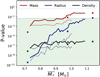 |
Fig. 8 Results of the moving sample analysis: P-value against the mean value of the stellar mass in the subsample. The red, blue, and black lines correspond to the mass, radius, and density distribution, respectively. The green region shows the statistically significant region, with P-values less than 0.05. The three stars of each color correspond to the P-values of the thirds of the population ordered by stellar mass. The dashed lines correspond to a sample of planets with masses below 100 M⊕. |
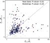 |
Fig. 9 Peas in a pod pattern for the orbital period spacing. The figure shows the period ratio of the outer pairs as a function of the period ratio of the inner pairs. The right figure shows the average radius of the pair against its period ratio. The red stars correspond to Solar System planets. |
2.7 Sample selection effect
Another relevant factor that should be considered when studying the similarity of planetary systems is the effect of the used catalog on the inferred results. It is common to set a limit on the relative uncertainty of the mass and radius measurement in order to discard the least accurate data. We therefore investigated the sensitivity of the results on the limits of the uncertainties on the measured mass and radius, and the results are shown in Table 1. We explored a range of uncertainties ranging from 50 to 16% in mass since lower values of the upper limits in uncertainties lead to samples with a small number of exoplanets. We set the limits for the radius uncertainties to be one-third of the mass uncertainties in order to have the same impact on the density uncertainty. We find that catalogs with more precise data lead to a weaker mass correlation between adjacent planets. However, this is linked to the previous result on the dependence on the mass limit, since giant planets tend to have lower relative uncertainties. In order to avoid this bias, we discarded planets with masses above 100 M⊕. Table 2 lists the dependence of the P-value and the R-value on the uncertainties on the sample of planets less massive than 100 M⊕.
We still find that catalogs with more precise data lead to weaker correlation between adjacent planets. As previously argued, this could be because of the smaller number of data points in the sample. We note that the P-values obtained when decreasing the limit on uncertainties are higher than those inferred when only removing points randomly. For example, when we decrease the uncertainties from  < 0.5 and
  < 0.16 to
  < 0.3 and
  < 0.1, the number of pairs decreases from 66 to 44 and the P-value increases from 4 × 10⁻¹⁰ to 4 × 10⁻⁶. However, when we randomly remove 22 pairs from the initial sample of 58, we infer a P-value between 9 × 10⁻⁹ and 6 × 10⁻⁷. Therefore, we conclude that the increase in the P-value is not caused by the increase in the number of points, and consequently the systems with more precise mass and radius measurements are less uniform, even after excluding gas giants. This is probably due to a selection effect since very low-mass planets tend to have higher uncertainties and tend to be more similar, as seen in Sect. 2.3.
Sensitivity of the P-value when analyzing the period ratio of the outer pairs as function of the period ratio of the inner pairs.
3 Uniformity in period spacing
In this section we focus on the aspect of period spacing. There are various studies that have investigated the orbital spacings of Kepler’s multiple system using the Titius-Bode relation (e.g., Lineweaver 2015; Huang & Bakos 2014), their clustering around theoretical stability thresholds (e.g., Pu & Wu 2015), and the spacing of Kepler planets in terms of the orbital period ratio (e.g., Lissauer et al. 2011; Steffen 2013; Steffen & Hwang 2015). Recently, Weiss et al. (2018) found that planets orbiting the same star tend to have regular orbital spacings, and Jiang et al. (2020) confirmed this pattern and concluded that such a correlation is unlikely to be caused by observational biases.
These results, however, correspond to different exoplanet samples and filtering criteria. In this section we investigate how the inferred uniformity in orbital spacing of planetary systems depends on the used data and the selection criteria. First, Jiang et al. (2020) only consider systems with multiplicities higher than four arguing that systems of lower multiplicities tend not to be dynamically packed, and therefore it is more likely to miss non-transiting planets. Second, Weiss et al. (2018) and Jiang et al. (2020) exclude period ratios of adjacent planets higher than four since in these systems the sensitivity to observe larger orbital periods may be incomplete. Finally, they only consider planets with radii below 6 R⊕.
In this section we do not use the planetary sample used in Sect. 2 since we aim to include more systems in our sample. Instead, we also include planets without mass measurements and do not put any constraint on the maximum radius uncertainty, which leaves us with 474 planetary systems and 1220 planets. The obtained period ratios of a planet pair against the next planet pair is shown in Fig. 9. We perform the same bootstrap test as before, and conclude that the inferred correlation cannot be explained by selection effects from observational biases. We note that systems with low period ratios of adjacent planets are significantly more uniformly distributed than the above mentioned sample because for systems with high period ratios there might not be any dynamical interaction between the planets, or perhaps it is simply due to observational bias.
We next explore the sensitivity of the results on the various choices typically made to filter the planetary samples. The results are listed in Table 2, where we show the dependence of the P-value on the upper limit of the period ratios for exoplanet samples with different upper limits on planetary radii. We show the results corresponding to systems with multiplicities higher than 2 and with multiplicities higher than 3 (as done by Jiang et al. 2020). We find that the results strongly depend on the period of adjacent planets. When we exclude the systems with the highest period ratios the P-value decreases very significantly along the whole range of PRmax tested. This result is expected since systems with lower period ratios have stronger dynamical interaction.
The effect of setting a limit on the maximum radius is less clear. When we set a lower radius limit the P-value increases, but this could be due to the smaller number of data points available in the sample. We analyze the dependence of the P-value on the number of data points, as previously done, and conclude that the increase in the P-value when reducing the number of data points could also be explained by the smaller number of data points. However, it is remarkable that the small sample with system of radii below 2 R⊕ has a P-value of 0.01, which cannot be explained by the number of data points. These systems with rocky planets are therefore more uniformly spaced than the systems with larger planets. Finally, the effect of the minimum multiplicity is also not conclusive. As we did for the radius limit, we find higher P-values that can be explained by the smaller number of data points in the sample.
4 Discussion and conclusions
In this paper we explored the similarity of planets within a multi-planet system. More specifically, we studied the peas in a pod pattern of radii, masses, densities, and orbital period ratios of adjacent planets, and confirm that their correlation has a physical origin. In addition, we quantified and compared the similarities in radius and mass. Finally, we explored whether different subpopulations of systems show different patterns, and how the results obtained depend on the exoplanet sample used.
Using a similarity metric defined as distance in logarithmic space, we find that planetary systems tend to be more similar in radius than in mass. This could be linked to the fact that the radius has a greater impact on the density, and hence on the planetary composition, than the mass. We also find a strong correlation between densities of adjacent planets. If the density is the main physical quantity that tends to be similar within a planetary system, it would explain the stronger similarity in radius than in mass. Detection biases are not expected to have a big influence on this result.
We also find that there is a sharp transition in the peas in a pod pattern of planets at 100 M⊕ and 10 R⊕. Systems with planets below these limits are significantly more uniform. As shown in the bootstrap trials, detection biases could lead to a less obvious peas in a pod pattern among large planets than among smaller ones. However, instead of finding a somewhat smooth transition in the uniformity of systems when transiting from small to large planets, we find two different regimes. It suggests that the physical processes governing the formation of planets with masses below 100 M⊕ clearly gives rise to adjacent planets with similar masses and radii, but not for more massive planets. We find that the P-values of the real data are 4.5σ and 12σ away from the bootstrap trials for the mass and radius distributions, respectively, when using the entire sample, and are 14σ and 16σ away when only planets less massive than 100 M⊕ are included. Interestingly, we do not find two regimes when analyzing the peas in a pod pattern in density: there is a rather clear correlation for all types of planets.
The dependence of the peas in a pod pattern with the planetary mass has to be treated with care and needs to be investigated further. First, exoplanet catalogs with more precise mass and radius measurements tend to be have fewer peas in a pod systemssince they contain a lower proportion of low-mass planets. Second, there is a clear dependency of the peas in a pod pattern on the stellar mass. Planetary systems around more massive stars tend to be less uniform in mass and radius, since they tend to host more massive planets. The peas in a pod pattern in density, instead, does not show a clear dependence on the stellar mass, which is expected due to its lack of dependence on the planetary mass.
Finally, the similarity trend orbital period spacing is clearly confirmed; we find that the strength of the correlation strongly depends on the maximum radius set for the planetary sample, which is often set arbitrarily in other publications. We also find that systems containing planets with low period ratios are more uniformly distributed, which may be indicative of a stronger dynamical interaction.
Ongoing and future space missions like TESS (Ricker et al. 2015), CHEOPS (Broeg et al. 2013), and PLATO (Roxburgh & Catala 2006), as well as ground-based radial velocity facilities like ESPRESSO (Pepe et al. 2014) will rapidly increase the number of characterized exoplanetary systems and will allow us to continue monitoring the systems analyzed in this study searching for missing planets. In addition, Gaia will perform high-precision astrometry and characterize missing planets in the
outer regions of multi-planet systems. This will lead to a more complete understanding of exoplanetary demographics and of the uniqueness of our own Solar System.
Appendix A Pearson Correlation
Figure A.1 shows the comparison of the measured P-value and R-value of the observed population of planets excluding planets more massive than 100M⊕ (dashed lines) with the results of 3000 bootstrap trials. We find that when we use a planetary sample with masses below 100M⊕, the calculated P-values of the real data are 14σ and 17σ away from the bootstrap trials for the mass and radius distributions, respectively. Figure A.2 shows the dependence of the P-value and R-valueon the number of pairs on the sample. It shows the evolution of these two values after randomly removing pairs.
Table A.1 shows the full list of similarities of the multi-planetary systems in our exoplanet sample. We include the similarities of the Solar System, inner Solar System, and outer Solar System for reference.
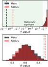 |
Fig. A.1 Calculated P-value (top) and R-value (bottom) corresponding to the correlation between the mass (black) or radius (red) of a planet and the mass or radius of the next farthest planet, excluding planets more massive than 100M⊕. The dashed lines correspond to the result from the exoplanet sample and the histograms to the results of 3000 bootstrap trials. The green region in the upper panel shows the statistically significant region where the P-value is smaller than 0.05. |
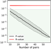 |
Fig. A.2 Dependence of the P-value and R-value on the number of pairs of the sample. The thick lines correspond to the median of the distribution after randomly removing pairs 1000 times, and the colored envelopes to the 1σ error. The green region in the upper panel indicates the statistically significant region, with P-value < 0.05. |
Similarities of the multi-planet systems in our exoplanet sample, based on the distance in the log Mp and log Rp spaces. Also shown the similarities of the Solar System as reference.
References
- Akeson, R. L., Chen, X., Ciardi, D., et al. 2013, PASP, 125, 989 [Google Scholar]
- Alibert, Y. 2019, A&A, 624, A45 [NASA ADS] [CrossRef] [EDP Sciences] [Google Scholar]
- Ballard, S., & Johnson, J. A. 2016, ApJ, 816, 66 [Google Scholar]
- Bashi, D., & Zucker, S. 2021, A&A, 651, A61 [NASA ADS] [CrossRef] [EDP Sciences] [Google Scholar]
- Borucki, W. J., Koch, D., Basri, G., et al. 2010, Science, 327, 977 [Google Scholar]
- Broeg, C., Fortier, A., Ehrenreich, D., et al. 2013, Eur. Phys. J. Web Conf., 47, 03005 [CrossRef] [EDP Sciences] [Google Scholar]
- Carter, J. A., Agol, E., Chaplin, W. J., et al. 2012, Science, 337, 556 [Google Scholar]
- Christiansen, J. L., Jenkins, J. M., Caldwell, D. A., et al. 2012, PASP, 124, 1279 [NASA ADS] [CrossRef] [Google Scholar]
- Ciardi, D. R., Fabrycky, D. C., Ford, E. B., et al. 2013, ApJ, 763, 41 [CrossRef] [Google Scholar]
- Fabrycky, D. C., Lissauer, J. J., Ragozzine, D., et al. 2014, ApJ, 790, 146 [Google Scholar]
- Fang, J., & Margot, J.-L. 2012, ApJ, 761, 92 [Google Scholar]
- Gilbert, G. J., & Fabrycky, D. C. 2020, AJ, 159, 281 [Google Scholar]
- Hadden, S., & Lithwick, Y. 2014, ApJ, 787, 80 [Google Scholar]
- Hadden, S., & Lithwick, Y. 2017, AJ, 154, 5 [Google Scholar]
- Hansen, B. M. S., & Murray, N. 2013, ApJ, 775, 53 [Google Scholar]
- Helled, R., Lozovsky, M., & Zucker, S. 2016, MNRAS, 455, L96 [Google Scholar]
- Howell, S. B., Sobeck, C., Haas, M., et al. 2014, PASP, 126, 398 [Google Scholar]
- Huang, C. X., & Bakos, G. Á. 2014, MNRAS, 442, 674 [NASA ADS] [CrossRef] [Google Scholar]
- Jiang, C.-F., Xie, J.-W., & Zhou, J.-L. 2020, AJ, 160, 180 [NASA ADS] [CrossRef] [Google Scholar]
- Kipping, D. 2018, MNRAS, 473, 784 [NASA ADS] [CrossRef] [Google Scholar]
- Latham, D. W., Rowe, J. F., Quinn, S. N., et al. 2011, ApJ, 732, L24 [NASA ADS] [CrossRef] [Google Scholar]
- Lineweaver, C. H. 2015, IAU General Assembly, 29, 2258465 [NASA ADS] [Google Scholar]
- Lissauer, J. J., Ragozzine, D., Fabrycky, D. C., et al. 2011, ApJS, 197, 8 [Google Scholar]
- Lissauer, J. J., Marcy, G. W., Rowe, J. F., et al. 2012, ApJ, 750, 112 [NASA ADS] [CrossRef] [Google Scholar]
- Lissauer, J. J., Marcy, G. W., Bryson, S. T., et al. 2014, ApJ, 784, 44 [NASA ADS] [CrossRef] [Google Scholar]
- Lozovsky, M., Helled, R., Pascucci, I., et al. 2021, A&A, 652, A110 [NASA ADS] [CrossRef] [EDP Sciences] [Google Scholar]
- Malhotra, R. 2015, ApJ, 808, 71 [NASA ADS] [CrossRef] [Google Scholar]
- Millholland, S. C., & Winn, J. N. 2021, ApJ, 920, L34 [NASA ADS] [CrossRef] [Google Scholar]
- Millholland, S., Wang, S., & Laughlin, G. 2017, ApJ, 849, L33 [NASA ADS] [CrossRef] [Google Scholar]
- Mills, S. M., Fabrycky, D. C., Migaszewski, C., et al. 2016, Nature, 533, 509 [Google Scholar]
- Mishra, L., Alibert, Y., Leleu, A., et al. 2021, A&A, 656, A74 [NASA ADS] [CrossRef] [EDP Sciences] [Google Scholar]
- Mullally, F., Coughlin, J. L., Thompson, S. E., et al. 2015, ApJS, 217, 31 [Google Scholar]
- Murchikova, L., & Tremaine, S. 2020, AJ, 160, 160 [NASA ADS] [CrossRef] [Google Scholar]
- Otegi, J. F., Bouchy, F., & Helled, R. 2020, A&A, 634, A43 [NASA ADS] [CrossRef] [EDP Sciences] [Google Scholar]
- Owen, J. E., & Campos Estrada, B. 2020, Astrophysics Source Code Library [record ascl:2011.015] [Google Scholar]
- Owen, J. E., & Murray-Clay, R. 2018, MNRAS, 480, 2206 [NASA ADS] [CrossRef] [Google Scholar]
- Pepe, F., Molaro, P., Cristiani, S., et al. 2014, ArXiv e-prints [arXiv:1401.5918] [Google Scholar]
- Petigura, E. A., Howard, A. W., Marcy, G. W., et al. 2017, AJ, 154, 107 [NASA ADS] [CrossRef] [Google Scholar]
- Pu, B., & Wu,Y. 2015, ApJ, 807, 44 [Google Scholar]
- Ricker, G. R., Winn, J. N., Vanderspek, R., et al. 2015, J. Astron. Teles. Instrum. Syst., 1, 014003 [Google Scholar]
- Rowe, J. F., Bryson, S. T., Marcy, G. W., et al. 2014, ApJ, 784, 45 [Google Scholar]
- Roxburgh, I. W., & Catala, C. 2006, IAU Joint Discuss., 26, 32 [Google Scholar]
- Steffen, J. 2013, The Architectures of Near-Resonant Kepler Planets, USA: NASA OSS Proposal [Google Scholar]
- Steffen, J. H. 2016, MNRAS, 457, 4384 [NASA ADS] [CrossRef] [Google Scholar]
- Steffen, J. H., & Hwang, J. A. 2015, MNRAS, 448, 1956 [NASA ADS] [CrossRef] [Google Scholar]
- Van Eylen, V., Albrecht, S., Huang, X., et al. 2019, AJ, 157, 61 [Google Scholar]
- Wang, S. 2017, Res. Notes Am. Astron. Soc., 1, 26 [Google Scholar]
- Weiss, L. M., & Petigura, E. A. 2020, ApJ, 893, L1 [Google Scholar]
- Weiss, L. M., Marcy, G. W., Petigura, E. A., et al. 2018, AJ, 155, 48 [Google Scholar]
- Xie, J.-W., Dong, S., Zhu, Z., et al. 2016, Proc. Natl. Acad. Sci., 113, 11431 [Google Scholar]
- Zhu, W. 2020, AJ, 159, 188 [NASA ADS] [CrossRef] [Google Scholar]
All Tables
Dependence of the Pearson’s P and R values on the uncertainty to our exoplanet sample with planets less massive than 100 M⊕.
Sensitivity of the P-value when analyzing the period ratio of the outer pairs as function of the period ratio of the inner pairs.
Similarities of the multi-planet systems in our exoplanet sample, based on the distance in the log Mp and log Rp spaces. Also shown the similarities of the Solar System as reference.
All Figures
|
Fig. 1 Orbital architectures of the 48 multi-planet systems in our sample with measurement uncertainties smaller than σM ∕M = 50% and σR ∕R = 16%, and that of the inner Solar System. In the left panel the colors of the points represent the logarithm of the radius of a planet divided by the radius of the previous one, and the systems are ordered by similarity in radius (defined in Sect. 2.2). In the right panel the same is represented, but for the mass. The circle size is proportional to the radius of the planet. |
| In the text | |
|
Fig. 2 Histograms of the distances |
| In the text | |
|
Fig. 3 Similarity in radius |
| In the text | |
|
Fig. 4 Mass (left) or radius (right) of a planet against the mass or radius of the next planet (farther from the star). The color of the dots represents the mass of the host star. The green stars correspond to the Solar System planets and the gray points to a bootstrap trial. |
| In the text | |
|
Fig. 5 P-value against the upper mass limit (blue) and upper radius limit (red) of the exoplanet sample. The dashed lines indicate the mass and radius at the minimum. |
| In the text | |
|
Fig. 6 Planetary density against the densities of the next planet farther from the star. The colors of the dots represent the effective temperature of the host star, and the gray dots correspond to a bootstrap trial. Pairs of planets orbiting around M dwarfs are represented by light blue triangles. The planets in the Solar System are indicated by the green stars. |
| In the text | |
|
Fig. 7 Calculated P-value (top) and R-value (bottom) corresponding to the correlation between the mass (black) or radius (red) of a planet and the mass or radius of the next farthest planet. The dashed lines correspond to the results from the exoplanet sample and the histograms to the results of 3000 bootstrap trials. The green region in the upper panel shows the statistically significant region, where the P-value is smaller than 0.05. |
| In the text | |
|
Fig. 8 Results of the moving sample analysis: P-value against the mean value of the stellar mass in the subsample. The red, blue, and black lines correspond to the mass, radius, and density distribution, respectively. The green region shows the statistically significant region, with P-values less than 0.05. The three stars of each color correspond to the P-values of the thirds of the population ordered by stellar mass. The dashed lines correspond to a sample of planets with masses below 100 M⊕. |
| In the text | |
|
Fig. 9 Peas in a pod pattern for the orbital period spacing. The figure shows the period ratio of the outer pairs as a function of the period ratio of the inner pairs. The right figure shows the average radius of the pair against its period ratio. The red stars correspond to Solar System planets. |
| In the text | |
|
Fig. A.1 Calculated P-value (top) and R-value (bottom) corresponding to the correlation between the mass (black) or radius (red) of a planet and the mass or radius of the next farthest planet, excluding planets more massive than 100M⊕. The dashed lines correspond to the result from the exoplanet sample and the histograms to the results of 3000 bootstrap trials. The green region in the upper panel shows the statistically significant region where the P-value is smaller than 0.05. |
| In the text | |
|
Fig. A.2 Dependence of the P-value and R-value on the number of pairs of the sample. The thick lines correspond to the median of the distribution after randomly removing pairs 1000 times, and the colored envelopes to the 1σ error. The green region in the upper panel indicates the statistically significant region, with P-value < 0.05. |
| In the text | |
Current usage metrics show cumulative count of Article Views (full-text article views including HTML views, PDF and ePub downloads, according to the available data) and Abstracts Views on Vision4Press platform.
Data correspond to usage on the plateform after 2015. The current usage metrics is available 48-96 hours after online publication and is updated daily on week days.
Initial download of the metrics may take a while.