| Issue |
A&A
Volume 658, February 2022
|
|
|---|---|---|
| Article Number | A164 | |
| Number of page(s) | 14 | |
| Section | Extragalactic astronomy | |
| DOI | https://doi.org/10.1051/0004-6361/202142090 | |
| Published online | 17 February 2022 | |
Waiting times between gamma-ray flares of flat spectrum radio quasars, and constraints on emission processes
Istituto di Astrofisica e Planetologia Spaziali – Istituto Nazionale di Astrofisica (IAPS-INAF), Via Fosso del Cavaliere, 100, 00133 Rome, Italy
e-mail: This email address is being protected from spambots. You need JavaScript enabled to view it.
Received:
25
August
2021
Accepted:
2
November
2021
Abstract
Context. The physical scenario responsible for gamma-ray flaring activity and its location for flat spectrum radio quasars is still debated.
Aims. The study of the statistical distribution of waiting times between flares, defined as the time intervals between consecutive activity peaks, can give information on the distribution of flaring times and constrain the physical mechanism responsible for gamma-ray emission.
Methods. We adopt here a scan statistic-driven clustering method (iSRS) to recognize flaring states within the Fermi-LAT archival data, and identify the time of activity peaks.
Results. We obtained that waiting times between flares can be described with a Poissonian process, consisting of a set of overlapping bursts of flares, with an average burst duration of ∼0.6 year and average rate of ∼1.3 y−1. For short waiting times (below 1 d host-frame) we found a statistically relevant second population, the fast component, consisting of a few tens of cases, most of them revealed for CTA 102. Interestingly, the period of conspicuous detection of the fast component of waiting times for CTA 102 coincides with the reported crossing time of the superluminal K1 feature with the C1 stationary feature in radio.
Conclusions. To reconcile the recollimation shock scenario with the bursting activity, we have to assume that plasma streams with a typical length of ∼2 pc (in the stream reference frame) reach the recollimation shock. Otherwise, the distribution of waiting times can be interpreted as originating from relativistic plasma moving along the jet for a deprojected length of ∼30−50 pc (assuming a bulk Γ = 10) that sporadically produces gamma-ray flares. In the magnetic reconnection scenario, reconnection events or plasma injection to the reconnection sites should be intermittent. Individual plasmoids can be resolved in a few favourable cases only, and could be responsible for the fast component.
Key words: radiation mechanisms: non-thermal / magnetic reconnection / shock waves / turbulence
© ESO 2022
1. Introduction
Blazars are the most luminous extragalactic objects observed in gamma rays. They emit from radio to teraelectronvolt (TeV). There is a general consensus that they are among the active galactic nuclei (AGNs) that are able to produce a jet approximately oriented along the polar axis. In particular, blazars are jetted AGNs for which the line of sight of the observer lies close to the jet axis (Urry & Padovani 1995).
Very Long Baseline Array (VLBA) images of AGN jets at 15 GHz show that jet geometry in the region from 102 to 103 pc from the core is approximately conical with an aperture of ∼1° (Pushkarev et al. 2017). Several jets have parabolic shapes on shorter distances.
Relativistic features (Lister et al. 2016; Hovatta et al. 2009) moving downstream the jet are observed. They do not fill the entire cross-section of the ejection cone (Lister et al. 2013). Their motion is not always ballistic, showing radial and non-radial acceleration.
According to the broad-line emission power with respect to the optical continuum (Urry & Padovani 1995), blazars are sub-divided into flat spectrum radio quasars (FSRQs, showing strong broad emission lines) and BL Lac objects (with weak or absent broad emission lines). The gamma ray observed from blazars is due to the Doppler-boosted emission from the jet. The mechanism responsible for gamma-ray emission is still a debated issue. The kind of accelerated particles (leptons, hadrons) that give rise to the gamma-ray emission, the accelerating engine, and its location are also controversial.
Particles can accelerate through the shock diffusive acceleration (Aller et al. 1985; Hughes et al. 1985; Blandford & Eichler 1987). In this model piston-driven shock originates blazar outbursts; the shock compresses and orders the upstream magnetic field, causing the electrons to accelerate though the Fermi mechanism and the emitted synchrotron radiation to be polarized.
Alternatively, Narayan & Piran (2012), Marscher (2013, 2014) proposed turbulence inside the jet as the accelerating mechanism. Flares are triggered by the passage of a turbulent relativistic plasma flow in a re-collimation shock, located at parsec scale from the central supermassive black hole (SMBH). The shock compresses the plasma and accelerates the electrons. The emission from a single turbulent cell is responsible for a rapid flare.
In magnetically dominated flows, magnetic reconnection driven by magnetic instabilities along the jet can efficiently accelerate particles (Zenitani & Hoshino 2001; Guo et al. 2014). Giannios (2013) found that magnetic reconnection events lead to the formation of plasmoids, whose emission overlaps in an envelope. Exceptional plasmoids can grow and produce fast flares that can be resolved from the envelope.
In leptonic models for FSRQ emission, the inverse-Compton on an external target photon field (EC) is often adopted to explain the gamma-ray emission from relativistic electrons (Maraschi et al. 1992). Seed photons can be the continuum and line emission from the broad-line region, or the black-body emission from dusty torus. There is general agreement that if this is the emission mechanism, the flare peak-luminosity is proportional to the energy density of the external photon field (Dermer et al. 1997). It has also been found that electrons radiating via the inverse-Compton mechanism on external photon fields dissipate their kinetic energy with a cooling time that is inversely proportional to the energy density of the target field (see e.g. Felten & Morrison 1966).
Alternatively, synchrotron radiation produced during flares is the target photon field for inverse-Compton scattering, known as the synchro-self Compton (SSC) model (Maraschi et al. 1992; Marscher & Bloom 1992). This model is often invoked to model the gamma-ray emission of BL Lac objects. Protons accelerated within the jet could reach the threshold for photo-pion production. In this model, the proton-synchrotron, the π0 → γγ decay are responsible for jet gamma-ray emission (hadronic model, see. e.g. Bottcher et al. 2013).
Casadio et al. (2015, 2019) showed that several gamma-ray flares of FSRQs can be associated in time with superluminal features crossing stationary features along the jet observed at 43 GHz. They associated the stationary feature C1 that they observed in the jet of CTA 102 with a recollimation shock. In particular, Casadio et al. (2019) argued that the interaction of the superluminal structure K1 with recollimation shock C1 generated gamma-ray flaring activity from the end of 2016 to the beginning of 2017.
Larionov et al. (2020) discussed a similar scenario for 3C 279 observed from radio to gamma-ray wavelengths for the years 2008–2018. They noted that the evaluation of crossing-time of radio steady features by superluminal features have large uncertainties, thus the association of crossing-time with gamma-ray activity had a good chance of being spurious.
In this paper we study the flaring activity in gamma rays of FSRQs contained in the third Fermi-LAT catalogue (3FGL, Acero et al. 2015). In particular, we focus on the waiting times between activity peaks, defined as the time interval Δt between two consecutive activity peaks (see Wheatland & Litvinenko 2002, for a description of waiting times). The study is performed over 9.5 y of data, from the beginning of the Fermi-LAT operation (Atwood et al. 2009) up to the failure of a solar panel actuator. During this period of whole-sky survey, the monitoring with Fermi-LAT can be considered continuous, with the satellite scanning each region of the sky approximately every two to four orbits. Other authors (see e.g. Abdo et al. 2010; Nagakawa & Mori 2013; Sobolewska et al. 2014; Meyer et al. 2019; Tavecchio et al. 2020) studied blazar variability in gamma rays, focusing on gamma-ray light curves, rather than on the waiting time between activity peaks. Instead, we disentangle the investigation of gamma-ray variability in a study of a temporal distribution of waiting times (this paper) and a study of correlated distribution of peak luminosity and flare duration (discussed in a forthcoming paper).
It is useful to report here some useful distributions concerning waiting times. If we assume a uniformly distributed sample of events within a period of duration T, the distribution of Δt between consecutive events inside the period is exponential  (where τ is the mean waiting time between consecutive events). Moreover, the time interval Δt = ti + k − ti between the events i and i + k of the time-ordered list of events is Erlang distributed with probability distribution function
  . If, for some reason, we do not detect an event, the observed distribution of waiting times between detected events deviates from an exponential distribution. For very short waiting times (Δt → 0) the exponential trend is restored because the contribution of the Erlang distribution for k > 1 tends to 0.
2. Analysis method
We investigated the Fermi-LAT archival data, prepared data using the standard Fermi Science Tools (v10r0p5), and used the PASS8 response functions. We applied standard analysis cuts, and selected SOURCE class events (evclass = 128) within 20° of the investigated source using gtselect. We applied a zenith angle cut of 90° to reject Earth limb gamma rays. We identified activity periods of each source using the iterated short range search (iSRS) clustering method (Pacciani 2018) applied to 9.5 years of gamma-ray data.
It is useful to recall some definitions and the method used in Pacciani (2018). For each source an extraction region is chosen for every event; it corresponds to the 68% containment radius (the containment radius depends on Energy and event type). Gamma-ray events within the chosen extraction region around the source catalogue position are selected. We can evaluate the cumulative exposure of the instrument to the source from the start of the Fermi-LAT operation to the time of arrival of each gamma-ray photon; gamma-ray events are time tagged, and also (cumulative) exposure tagged. Clusters of events are obtained applying the iSRS procedure in the cumulative exposure domain, not in time domain (because the exposure to the source varies with time). From the dataset of each source, the set of clusters obtained with the iSRS procedure are statistically relevant; we used a threshold for chance probability Pthr = 1.3 × 10⁻³, and a tolerance parameter Ntol = 50. This set is a tree, called the unbinned light curve. The clusters representing the activity peaks are the leaves of the tree.
For each leaf, a peak time, and peak flux are identified. The branches of the tree ending with a leaf are the detected flares of the unbinned light curve; detected flares are described by a branch that contains at least the leaf.
As an example, we show in Fig. 1 the unbinned light curve for PKS 1510–08. The horizontal segments are the relevant clusters of events obtained with the iSRS procedure. They are described by the starting time, the duration, and the density of events in the exposure domain (e.g. by the average photometric source flux for the period of time subtended by the cluster). When the background is not subtracted the flux is denoted by FSRC + BKG. The vertical bars represent the errors on the flux estimate. Clusters are organized in a tree hierarchy. Each cluster is statistically relevant with respect to its parent. Assuming that events in a parent cluster are uniformly distributed, there is a probability ≤Pthr that the child cluster is obtained by chance from the parent cluster. The cluster at the base of the tree is the root.
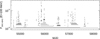 |
Fig. 1. Unbinned light curve (Pacciani 2018) for PKS 1510–08, obtained with Pthr = 1.3 × 10⁻³. Horizontal lines are the statistically relevant clusters. The set of statistically relevant clusters is a tree, and a hierarchy among clusters exists. For each child cluster there is a probability ≤Pthr to be obtained starting from its parent cluster by chance. Vertical bars are the errors on the flux estimate. Background is not subtracted. |
We define a fully resolved flare as one for which the branch contains the leaf and at least one other cluster, and we define a resolved flare as one for which the branch contains the leaf alone.
Photometric flux at peak  was extracted for resolved flares. Photometric flux at peak
  and flare duration measured by the full width at half maximum (FWHMflare) were extracted for fully resolved flares.
We also applied the standard analysis tools to extract flux ( , based on likelihood method) and its significance (from TS statistic) of the source for the periods of activity identified by the leaves.
All photometric methods suffer positional pile-up due to the instrumental point spread function (PSF) and the presence of nearby sources. The method adopted here to study source variability is photometric, and it is sensitive to variability of the positional pile-up. To disentangle flares coming from contiguous sources, we reject flares with a ratio  , or with TS < 9.
We prepared the sample used in this study with this method. Some contamination remains in the sample from contiguous sources, and some systematics could affect the results that we show. We account for the systematic effects by comparing the results varying the threshold on Rphoto2like from 1.1 to 2.
3. Samples of activity peaks
We selected gamma-ray emitting FSRQs, starting from the third Fermi-LAT catalogue (3FGL). We identified gamma-ray flaring periods from the Fermi-LAT archival data within the period 2008 August–2018 February.
Because the gamma-ray analysis of sources at low galactic latitude is a cumbersome task, especially if photometric methods are adopted, we restrict the investigation to the high latitude FSRQs (b > 15°) contained in 3FGL. To avoid contamination from spurious sources within the 3FGL, we took into account bright catalogue sources, with a TS statistic ≥49. With these restrictions we investigated 335 FSRQs.
We obtained two samples of activity peaks based on the energy range of gamma-ray photons. A first sample is obtained selecting gamma-ray events with an energy E > 300 MeV (300 MeV sample). Starting from the sources with at least two flares in the 300 MeV sample, we also prepared a sample of activity peaks from the gamma-ray events with E > 100 MeV (100 MeV sample).
To resolve in time two close flares, a large sample is needed (Pacciani 2018). In Appendix C, we show the effect on simulated samples. For this reason we make use of the 100 MeV sample in this paper.
4. Results
In this paper we always report waiting times, rates, and duration in the host galaxy reference frame, except where explicitly written.
We performed several uniformity and unimodality tests on the sets of activity peaks of the apparently loudest sources (the sources with the largest number of detected flares). They are reported in Table 1. Under the assumption that the Fermi-LAT regularly scanned each sky position, the distribution of flaring times cannot be considered either uniform or unimodal.
Tests for time distribution of flares on sources showing Nflares > 15 in the 100 MeV sample.
The obtained distribution of waiting times (with logarithmic bin) is shown in Fig. 2 (left column), while in the right column the same distribution divided for the binsize is shown; the last distribution is proportional to ρ(log(Δt))e−Δt. Fitting functions are superimposed to the data. The fitting function shown as the dashed line represents a set of overlapping bursts of flares (the multi-loghat distribution described in Appendix A). The parameters of the fitting functions are reported in Table 2. The multi-loghat distribution is a Poissonian process: the events within a burst are uniformly distributed. There is good agreement between data and the multi-loghat model for Δt larger than 1 day. For short waiting times (Δt → 0) the multi-loghat distribution and all the distributions based on Poisson processes (see e.g. Wheatland 2000) shows an exponential profile  (where τ is the typical timescales of the distribution). Thus, the fitting distribution reported in the right column of Fig. 2 tends to a constant. Experimental data show this trend (Fig. 2), but for Δt < 1 d data deviate from the typical Poissonian profile, and show an increasing trend for reducing values of Δt.
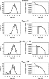 |
Fig. 2. Distribution of waiting times between gamma-ray flares of FSRQ detected with the iSRS method (100 MeV sample). Left columns: distribution (ρ(log(Δt)) of log(Δt). Right columns: same distribution divided by the bin size; this new distribution is proportional to ρ(log(Δt))e−Δt. The top row reports the distribution for all the sources. The other rows report the distribution of waiting times for sources selected on account of detected flares (from top to bottom): Nflares ≤ 9, 10 ≤ Nflares ≤ 19, Nflares ≥ 20. Solid histograms represent the data, dashed curves the multi-loghat fitting function. The solid grey line in the top row is the composite model obtained adding a Poissonian process to the multi-loghat fitting function. |
Fitted values of the parameters of the multi-loghat, multi-loghat + Poissonian, multi-pow, and multi-pow + Poissonian distributions for the temporal distribution of flares.
We can regard the distribution as a combination of two distributions: a multi-loghat distribution and another one acting on short waiting times (see e.g. Aschwanden & McTiernan 2010, for the study of solar flares with ISEE-3/ICE). We call the second distribution the fast component, and we call multi-loghat + Poissonian the composite distribution.
Only a few tens of waiting times can be ascribed to the fast component, thus we cannot establish a reliable functional form with this dataset. We simply added a further Poissonian term responsible for short waiting times. The resulting fitting function for the whole data sample is shown in Fig. 2 (top row) and its parameters are reported in Table 2. The observed fraction of short waiting times is reported as Rfast observed in Table 2. The reduction of the Cash estimator obtained adding the fast component tells us that the fast component is statistically relevant.
We also tested other fitting functions for the temporal distribution of flares. We obtained an intermediate result in terms of the Cash estimator with the multi-pow distribution function (defined in Appendix A). The results are reported in Table 2. The multi-pow distribution does not reproduce the trend observed for Δt < 1 d. It gives better results with respect to the multi-loghat distribution, because for the multi-pow distribution, the function ρ(log(Δt))e−Δt rises while Δt decreases. Thus, it roughly reproduces data with short Δt.
We also tried to fit with another two-component distribution: the multi-pow + Poissonian (defined in Appendix A, with five parameters). Results are reported in Table 2. With this distribution we obtained the best Cash estimator, but it is statistically comparable with the value obtained with the multi-loghat + Poissonian. The multi-loghat + Poissonian and the multi-pow + Poissonian distributions (with five parameters) are the statistically relevant models; they give ΔC = −10.0, and ΔC = −11.5 respectively with respect to the multi-pow distribution (with three parameters).
We show in Appendix C that the resolving power depends on the temporal distance between flares, and on peak fluxes. Moreover, the apparently loudest sources are also the brightest ones. Thus, we expect that the apparently loudest sources show the largest amount of short waiting times. This trend shows up in Fig. 2. We show for a physical scenario that close flares could not be resolved individually (pile-up effect), causing a reduction of short waiting time statistics.
4.1. Case study: CTA 102
We note that the majority of short waiting times (Δt < 1 d) come from CTA 102. They are mainly grouped around MJD 57738 and MJD 57752. The unbinned light curve of the source for a 100 d period (obtained with a chance probability threshold Pthr = 1.3 × 10⁻³) is reported in Fig. 3. The peculiar distribution of waiting times is shown in Fig. 4.
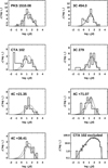 |
Fig. 3. Unbinned light curve (Pacciani 2018) for CTA 102 obtained for E > 100 MeV (see Pacciani 2018, for a detailed explanation), and zoom-ins of the relevant periods. The horizontal segments represent statistically relevant clusters of events obtained with the iSRS procedure. They are described by duration, average photometric flux, and median time (or by starting time). Vertical lines are the error bars on the flux estimate. The set of clusters form a tree called unbinned light curve. Background is not subtracted. |
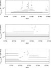 |
Fig. 4. Distribution of waiting times for the apparently loudest sources in the sample, and for the whole sample (excluding CTA 102, right bottom plot). Solid histograms represent the data, dashed curves the multi-loghat fitting function evaluated for the whole data sample. For single sources the grey lines represent the multi-loghat fitting function evaluated for each source separately, with parameters reported in Table 3; the fit is performed for Δt > 0.3 d to reduce the contribution of the fast component. |
The unbinned light curve can be compared with the results reported in D’Ammando et al. (2019) and in Meyer et al. (2019). There are two fast flares that were fully resolved with the iSRC: the first flare peaks at MJD 57752.50 with a duration of 7.8 h (FWHM, observer frame), the second flare peaks at MJD 57752.83 with a duration of 1.5 h (FWHM, observer frame). A further fast flare is fully resolved adopting a Pthr = 2.3%; it peaks at MJD 57738.00, with a duration of 2 h. We also note that in the 0.3 d period between MJD 57738.2 and MJD 57738.5 the iSRS procedure resolves a set of four peaks (but the statistics do not allow the flares to be fully resolved). Thus, the average duration of each flare of the set is ≤0.1 d. Similarly, in the 1 d period between 57751.8 and 57753.0 there are three resolved and two fully resolved flares, for an average flare duration of ≤0.2 d.
We discuss in Appendix C the temporal pile-up. In particular, flares with a temporal distance of 0.1 d could be resolved if their flux exceed 2 × 10⁻⁵ ph cm−2 s−1 (Fig. C.1). This is the case for the resolved flares just mentioned. We cannot exclude that the tail preceding the peak at MJD 57738.00 is due to the pile-up of several flares with a trend of decreasing waiting times, or a trend of increasing flux. There is a hint of a complex structure from the 12 h binned light curve reported in D’Ammando et al. (2019).
4.2. Peculiar source: S4 0218+35
The sample of sources we analysed also includes S4 0218+35, a blazar with a gravitational lens along the line of sight. The effect of the gravitational lens shows up in the distribution of waiting times reported in Fig. 5. They cluster around Δt ∼ 11 d (observer frame), in close agreement with the waiting time of delayed echo measured with VLA (Biggs et al. 1999; Cohen et al. 2000) and with the gamma-ray data itself (Barnacka et al. 2016).
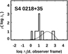 |
Fig. 5. Distribution of waiting times for the lensed source S4 0218+35 (observer reference system). Solid histogram represents the data, dashed curve the fitting function. |
4.3. Remaining sources
In order to reduce the signal from the short component, we performed a further investigation of waiting times distribution removing CTA 102 from the sample. We evaluated several fitting functions. The relevant ones are described in Appendix A.
In Fig. 2 we show the fit with the multi-loghat distribution. It gives a satisfactory description of data; the results are reported in Table 2.
The joint confidence region for the burst rate and duration parameters is reported in Fig. 6 for the multi-loghat distribution (top panel). Fitting the multi-loghat function to the waiting time distribution generates correlated estimates of the two parameters.
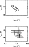 |
Fig. 6. Multi-loghat fit of the waiting times for the 100 MeV sample, and comparison with results reported in Jorstad et al. (2017). Top panel: joint confidence region for rburst and τburst (for the whole 100 MeV sample, excluding CTA 102). The parameters for the minimum of the Cash estimator are reported with a cross. Contours are reported for 90% and 99% confidence levels. The resolved superluminal features ejection rate and fading time observed at 43 GHz (Jorstad et al. 2017) are reported with a diamond symbol (average values). Bottom panel: rburst and τburst (in black) obtained by fitting the multi-loghat distribution to the data of single sources (for the apparently loudest sources in our gamma-ray sample). For comparison, the apparent ejection rate and fading times for each FSRQs reported in Jorstad et al. (2017) are also reported (in grey). |
The Cash estimator variation from a uniform to a multi-loghat function is ΔC = −105.8, in favour of the multi-loghat distribution.
We tested other fitting functions for the temporal distribution of flares. We obtained slightly better results with the multi-pow distribution function. The results are reported in Table 2. Furthermore, we obtained that if fitting is limited to Δt > 1 d, the Cash estimators for multi-loghat and multi-pow distributions become very similar.
Changing the pole position into the middle of the burst for the multi-pow does not produce a better value of the Cash estimator. Moreover, using multi-pow-smooth instead of a multi-pow does not give a better Cash estimator. In Fig. 4 we show the waiting times distribution of the apparently loudest sources in our sample, together with the multi-loghat fitting function, evaluated at the minimum of the Cash estimator for the whole 100 MeV sample, except CTA 102. A small amount of short waiting times are well outside the fitting distribution of single sources; the fast component arises also for sources other than CTA 102, but activity peaks that are close in time are resolved only for extremely bright flares. This is the case for 3C 454.3, flaring around MJD 55517–55521, and for 3C 279, flaring around MJD 57189.
The fast component does not show up in the distribution of waiting times accumulated for all the sources (except CTA 102). We show that for realistic simulations (taking into account flare duration, and exposure variation with time), some pile-up effect appears for Δt shorter than several days. The net effect is a reduction of statistics for short waiting times. We speculate that the cumulative distribution reported in Fig. 4 (right bottom plot) does not show the pile-up effect because the fast component compensates for the reduction of statistics for short waiting times.
In Table 3, in Figs. 4 and 6 (bottom panel) we report the results obtained fitting the multi-loghat model to the waiting time distributions for single sources. Due to the limited sample size, we fitted the model to the data of single sources fixing the parameter σlog(τ) to the value obtained by fitting the multi-loghat model to the accumulated distribution (σlog(τ) = 0.36). Moreover, we restricted to Δt ≥ 0.3 d to minimize the contribution of the fast component to the single-source samples.
Fitting parameters of the multi-loghat model for the temporal distribution of flares.
5. Discussion and conclusion
5.1. Distribution of waiting times for a non-ideal instrument
In the previous section we studied the waiting time distribution for an ideal instrument. In order to investigate the effect of the exposure variation with time for each source, the gaps between observations of the Fermi-LAT, and the pile-up effect, we performed detailed simulations taking into account the exposure to each source. We investigated three cases:
-
(a)
Flares uniformly distributed within the observation period of 9.5 y;
-
(b)
Time distribution of flares follows the multi-loghat distribution;
-
(c)
Time distribution of flares follows the multi-loghat distribution.
For cases a and b we extracted the logarithm of the Doppler factor of accelerated electrons log(δflare) with a gamma distribution, with mean = 1, and variance = 0.045 (see the best-fit intrinsic jet properties obtained for the 1.5 JyQC quasar sample in Lister et al. 2019). Flare duration is proportional to  .
.
The observer’s line of sight with respect to the jet axis, and the bulk Lorentz factor of the emitting feature affect the observed peak flux, flare duration, and waiting times between flares. The amount of the effect depends on the emission process responsible for gamma-ray emission, and on the physical scenario responsible for flaring activity. To account for this, we also studied a simple geometry for the emitting source (case c).
For case c the flares are uniformly generated within the burst. Flares within each burst of activity have all the same Lorentz factor, and the same orientation (of the moving blob) with respect to the jet axis: it is uniformly extracted within a cone of aperture 1° around the jet axis. The line of sight is uniformly extracted within a cone of 8° aperture from the axis of the blazar jet. For each flare, peak luminosity and flare duration FWHM are anti-correlated. We explored two sub-cases: (1) peak luminosity is proportional to  (EC leptonic model, see e.g. Dermer et al. 1997) and the FWHM is proportional to
  (light crossing time prevails on cooling, case clct), and (2) the flare duration FWHM is proportional to
  (cooling time prevails, case ccooling, see e.g. Pacciani 2014). The burst rate is a constant for all the sources. We did not try to reproduce the fast component of waiting times, but only the multi-loghat component. This last case imposes that all the flares from the same burst have the same Doppler factor, and thus have a large coherence.
We modelled peak luminosity and flare duration of simulations with a parametric distribution, whose parameters were obtained by fitting the models to the peak luminosity and duration of detected flares. Further details of the models will be described in a dedicated paper. For all the models, flare shape was modelled according to Eq. (7) in Abdo et al. (2010), and converted in a temporal distribution of gamma rays detected by an ideal telescope. We also tried to model the flare temporal profile with Gaussian and gamma distributions, obtaining similar results. Finally, each gamma ray is randomly accepted or rejected according to the real exposure to the source. Exposure was evaluated for temporal bins of 86.4 s. Once the time series were obtained for each source, we applied the iSRS procedure to extract flares from simulated data (the same procedure used to extract flares from real data).
For case a, we performed 100 simulations. We fitted the simulated waiting times distribution with with a uniform distribution and with a multi-loghat distribution. The multi-loghat distribution approaches a uniform distribution for burst rates much larger than the flaring rate within a burst, and we can successfully fit the uniformly distributed samples using a multi-loghat fitting function. Due to the telescope exposure variation with time to each source, the final sample of recognized flares could mimic a multi loghat distribution of waiting times. We obtained for case a (uniformly distributed flares) that the absolute variation of the Cash estimator from uniform to multi-loghat fitting function is |ΔC|< 3. We already found for real data that the variation of the Cash estimator from uniform to multi-loghat fitting distribution is ΔC = −105.8. Thus, we can reject the hypothesis that (for real data) uniformly distributed flares (in times) could mimic a multi-loghat distribution of waiting times (due to exposure variation with time). We find, instead, that fitting the multi-loghat function to the waiting time distributions obtained simulating cases b and c, the fitted bursting rate and duration corresponded to the simulated bursting rate, and duration of generated samples. So, the fitting procedure and results obtained fitting the multi-loghat to the data is validated with simulations.
We note that for case c the pile-up effect is reduced with respect to case b. For case c flares within the same burst are highly correlated because they all have the same Lorentz and Doppler factor. From the detailed simulations we obtained that temporal resolving power reduces to  at Δt = 4 d, 2 d, and 1.5 d, respectively, for case b, case ccooling (cooling time prevails), and case clct (light crossing time prevails).
The detailed modelling cannot reproduce exactly the same number of detected flares, but we obtained that the revealed number of simulated flares for each source was at most within a factor of ∼2 with respect to real data. The comparison of the detailed simulation (case clct) with the data is shown in Fig. 7.
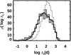 |
Fig. 7. Distribution of waiting times for data (grey line), simulated case a (uniformly distributed flares, thin dashed line), and simulated case clct (light crossing time prevails, black continuous line). |
The comparison was performed excluding CTA 102 from the 100 MeV sample. The waiting times obtained from the simulated time series reproduce the behaviour of the data. Some discrepancy remains for short waiting times (Δt < 3 d). With the detailed modelling, the pile-up effect occurs, suppressing the statistics for short waiting times. Moreover, the model does not try to reproduce the fast component acting on short timescales.
To summarize, a set of superimposing bursts of activity is able to reproduce the data. There is a suppression of statistics for short waiting times. Depending on the physical scenario, this suppression starts at Δt ∼ 1.5−4. The observed waiting time distribution for all the sources (CTA 102 excluded) reported in Fig. 2 does not show suppression. We guess that the fast component compensates for the pile-up suppression.
We could expect that gamma-ray FSRQs selected in this paper should have a broad distribution of the jet axis with respect to the line of sight, affecting the observed peak flux, flare duration, and waiting times between flares. As a results the accumulated distribution of waiting times should also be broad, due to the different viewing angles among sources, possibly washing out the multi-loghat time distribution proposed to fit the results. Instead, the flare luminosity dependency upon the Doppler factor strongly mitigate the effect for flux limited samples.
Flaring emitting regions, moving along a trajectory (that we identify with a flare direction) that is at a large angle with respect to the line of sight, usually remain undetected in gamma rays because of the dependency of the flaring luminosity Lγ upon the Doppler factor (Lγ ∝ δ4 + 2α for the external Compton, Lγ ∝ δ3 + α for the synchrotron emission, see e.g. Dermer et al. 1997). This suppression effect combines with the low probability of observing flares from electrons with bulk motion aligned with the line of sight. As a result, the viewing angle distribution for gamma-ray detected flares should be peaked at an intermediate value between 0 and the critical angle  . The distribution of viewing angles of gamma-ray detected flares (obtained simulating the simplified scheme ccooling where the bulk direction of the flare emitting electrons coincides with the knot direction) is reported in Fig. 8 (top panel).
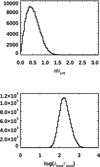 |
Fig. 8. Statistical distribution of relevant quantities obtained simulating case ccooling. To produce the histograms, the observer line of sight with respect to the jet axis was generated uniformly within a cone of aperture 30°. Top panel: distribution of viewing angles of gamma-ray detected flares. Bottom panel: distribution of Γknotδknot for gamma-ray detected flares. |
This circumstance strongly reduces the broadening of the accumulated waiting time distribution. Suppression was also investigated for flux-limited radio samples, with jet viewing angle distribution peaking at about half of the critical angle (see e.g. Vermeulen & Cohen 1994; Lister & Marscher 1997). A further suppression effect for gamma-ray detected blazars was also found in Savolainen et al. (2010), and in Pushkarev et al. (2017) (see their Fig. 15) reporting the distribution of jet viewing angles of the Mojave Radio sample for Fermi-LAT detected and for Fermi-LAT not detected AGNs. Our sample shows strong suppression at large viewing angles because it is obtained starting from Fermi-LAT detected FSRQs for which we revealed flaring activity. Thus, the accumulated distribution of waiting times between flares that we studied here is obtained for sources with a narrow angle between the line of sight and the jet axis. The simulated cases clct and ccooling show this suppression effect, and take into account the non-monochromatic distribution of the bulk Doppler factor of travelling knots (see Lister et al. 2019).
In the case of uniformly distributed flares within a burst of activity, we expect for each source a waiting time distribution ρ(log(Δt))e−Δt with a flat tail for short waiting times. As a result, the accumulated distribution (obtained accumulating waiting times for all the sources) should still have a flat tail for short waiting times, irrespective of the differences of burst rate and duration among sources.
5.2. Constraints on gamma-ray emission models
Jorstad et al. (2017) and Casadio et al. (2019) argued that gamma-ray flares could be associated with superluminal moving features crossing stationary features along the jet. If this is the case, the burst activity (which we revealed from waiting times between activity peaks) could be associated with plasma streams relativistically moving along the jet, and crossing a steady feature along their path. Assuming a stream with Γstream = 10, its typical length (in its reference system) measured along the jet is  .
.
Alternatively, we could assume that a travelling perturbation or a travelling knot is responsible for the bursting activity. We could assume that in this case the direction of accelerated particles is highly correlated with the direction of the travelling knot (corresponding to case c). We can correlate the duration of the observed burst with the travelled length lknot of the superluminal feature:
 (1)
(1)
In this scenario the viewing angle of the jet axis varies from source to source, and the Lorentz factor of moving knots is not monochromatic. Adopting the proposed case c, the distribution of Γknotδknot for gamma-ray detected flares can be evaluated with simulations. It is reported in Fig. 8 (bottom panel) assuming the mean Lorentz factor for the moving feature is Γknot = 10. We obtained a distribution of log(δknotΓknot) with mean value ∼2.26 and root mean square broadening ∼27%; thus, lknot is 30−50 pc. We note that, on account of Eq. (1) and of the spread of log(δknotΓknot), the viewing angle variation from source to source, and the distribution of Γbulk could be responsible, at least partially, for the spread of τburst reported in Table 2 (parameter σlog(τ) of the multi-loghat distribution).
We can compare the achieved results with the VLBA observations reported in Jorstad et al. (2017). In their Table 7 they report the fading time τ43 GHz for moving features observed at 43 GHz.
We report in Fig. 9 the τ43 GHz distribution and emission rate for the resolved superluminal features observed at 43 GHz (see Fig. 4 in Jorstad et al. 2017). The mean value for log (τ43 GHz(y)) of the fitting logarithmic distribution is −0.50 ± 0.02, and the standard deviation is 0.22 ± 0.02. It is tempting to associate the distribution of fading time of moving features, with the distribution of the duration of bursts of flares found in this paper and reported in Table 2. The comparison is reported in Fig. 6. Our results agree with the knot emission rate and with the fading time (within a factor of two) of knots observed at 43 GHz (Jorstad et al. 2017).
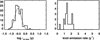 |
Fig. 9. Distribution of relevant parameters for the resolved superluminal features observed at 43 GHz. Left panel: fading time (reported in Table 4 in Jorstad et al. 2017) (log scale). Right panel: Ejection rate (from Table 5 in Jorstad et al. 2017). |
As the knot travels away from the SMBH, we expect a significant reduction in peak flux of the emitted flares. Both the external magnetic field B and the energy density of the external radiation field uext decrease along the travelled path ( , and
, and  , with d the distance of the emitting zone from the SMBH). Thus, the peak flux of flares generated along the travelled path follows the decreasing trend with d in optical (synchrotron emission) and in gamma rays (assuming EC emission). We note that the magnetic field reduction with the distance from the SMBH (and electron cooling) should also affect the fading time evaluated from radio luminosity of superluminal features (Jorstad et al. 2017). Homan et al. (2015) showed that radio features accelerate for deprojected distances of up to ∼100 pc from the central SMBH. If flares are emitted while knots still experience acceleration, the enhancement of Γknot could partially compensate the reduction of energy density of the external photon field.
Finally, in magnetic reconnection scenarios (see e.g. Giannios 2013), reconnection events can be triggered by magnetic instabilities such as kink instabilities (Begelman 1998; Spruit et al. 2001) or magnetic field inversions at the base of the jet (Giannios & Uzdensky 2019). We speculate that the bursting activity we reveal could be generated by intermittent magnetic instabilities or by intermittent flux of plasma; instability phases of the magnetic structure of the jet or the plasma injection to the reconnection sites should have a typical timescale of ∼0.6 y.
Sironi et al. (2016) obtained that plasmoids can be produced continuously (plasmoid chains) if fresh plasma is added to the system. Due to the limited flare resolving power of the Fermi-LAT, we are rarely able to resolve plasmoid emission from the envelope (see e.g. Christie et al. 2019). Thus, the activity peaks we observe in gamma rays correspond to the envelope emission from reconnection events. If this is the case, reconnection events must be uniformly produced in time during the development of magnetic instabilities. Moreover, we could associate the fast component with the rare cases for which we are able to resolve plasmoids within the envelope (when the jet axis and reconnection layer are almost aligned with the line of sight). In this physical scenario the orientation of the reconnection layer differs for each reconnection event (such as in simulated case b), but plasmoids from the same reconnection event emit along the same direction.
5.3. The fast component and the gamma-ray data of CTA 102
We observed a few tens of short waiting times (for waiting times < 1 d), mainly detected for CTA 102. The typical timescale of this component is ∼1 h. The detailed simulations, performed taking into account the Fermi-LAT exposure to the source, and realistic duration of flaring activity show that the temporal pile-up of close-by flares acts for waiting times < 1.5−4 d. We did not try to study the distribution of the fast component in more detail with the simple fitting provided here. In fact, pile-up plays a major role. Moreover, the exposure to sources cannot be considered continuous for time periods below several hours. A study could be performed applying detailed modelling for particle acceleration and gamma-ray emission to the simulating chain.
A fast, white component, with similar timescale was found in the optical for two BL Lac objects (Raiteri et al. 2021a,b). Interestingly, the fast component shows up in CTA 102 gamma-ray data for the time interval for which the superluminal component K1 crosses the C1 stationary feature of the jet, and for this event, the scenario of acceleration of turbulent cells from a recollimation shock was proposed (Casadio et al. 2019).
Larionov et al. (2017) interpreted the CTA 102 period of activity differently. They argued that a superluminal knot changing its own orientation and moving along the line of sight from the end of 2016 to the beginning of 2017 (during the period of conspicuous detection of the fast component) can produce the observed flux and polarization trend in optical and radio. We note that the change in orientation could explain the quadratic correlation observed in the optical and in gamma rays (Larionov et al. 2017). It corresponds to a change in Doppler factor and then to a change in gamma-ray luminosity Lgamma-ray ∝ δ4 + 2α (with α the gamma-ray spectral index), and to a change in optical luminosity Loptical ∝ δ3 + α, according to Dermer et al. (1997) for EC and synchrotron emission respectively. The weak polarization observed on 2016 December 23 reported in Casadio et al. (2019) for the K1 superluminal feature, witnesses for an aligned direction of the K1 component toward the observer.
The change in orientation scenario causes a reduction of less than a factor of 2 in waiting times of gamma rays, but it is responsible for a large increase in flux, and thus the activity peaks can be temporally resolved with the Fermi-LAT (we already discussed the net effect in the results for CTA 102). Thus, at least for a short period of time, we were able to resolve in gamma rays the fast component flaring activity, due to turbulence or to the plasmoid chain in reconnection scenario.
6. Summary
In this paper we found that gamma-ray activity peaks of FSRQs are produced in bursts. The average duration of a single burst is ∼0.6 y, and the average burst rate is ∼1.3 y−1. These are averaged values obtained from the whole analysed sample. The temporal distribution of activity peaks within each burst can be approximated with a uniform distribution.
Our overall distribution of waiting times between activity peaks shows a statistically relevant fast component (with Δt < 1 d), that can be roughly modelled with a uniform distribution with a typical waiting time of ∼1 h. CTA 102 shows the large majority of the fast population. Once CTA 102 is removed from the whole sample, the cumulative waiting time distribution of all the remaining sources does not show clear evidence of the fast population. Several cases of short waiting times that can be ascribed to the fast component can be found in the waiting time distribution of single sources. We evaluated the pile-up effect on the waiting time sample and found that it must be relevant for waiting times shorter than 1.5−4 d, depending on the modelling. We guess that the fast component and the pile-up compensate for each other in the cumulative distribution of waiting times of the remaining sources. Thus, the fast component should act for waiting times shorter than 1.5−4 d.
It is worth mentioning that Raiteri et al. (2021a,b) found a statistically relevant white noise emerging for frequencies above ∼0.9 h−1 and ∼3.6 h−1 in the power spectral density analysis (PSD) of optical data of the BL Lac objects S4 0954+65 and S5 0716+714, respectively, observed with the Transiting Exoplanet Survey Satellite (TESS; Ricker et al. 2015) and the Whole Earth Blazar Telescope (WEBT1) organization (Villata et al. 2002).
Our finding can be applied to existing theoretical and phenomenological models. Narayan & Piran (2012), Marscher (2013, 2014) proposed that gamma-ray flares originate from the passage of turbulent plasma inside a recollimation shock. In this scenario the burst of activity that we found could be associated with the length of a superluminal plasma stream. We estimated a length of ∼2 pc in the stream reference frame (assuming a Lorentz factor of the stream Γstream = 10, and a characteristic recollimation shock length much shorter than the stream length in the host galaxy frame).
Instead, if flares are generated along the path of a superluminal moving perturbation (or knot), the average path length should be 30−60 pc (assuming that the Lorentz factor of the superluminal feature is Γknot = 10). This scenario is not compatible with the 1/d2 scaling of the energy density of the magnetic and external photon field in leptonic models (with d the distance of the superluminal feature from the SMBH). The effect on emission of the 1/d2 scaling of external fields could be partially mitigated if the superluminal feature accelerates along its path.
Finally the reconnection particle accelerating scenario (Giannios 2013) divides the acceleration mechanism in the generation of reconnection events, and in the plasmoid-chain grown within each reconnection event (Sironi et al. 2016). In this scenario, we should associate the bursting activity to the jet magnetic field instabilities (which generate reconnection events) or to the plasma injection to the reconnection sites, and the fast component to the gamma-ray emission from the plasmoid chain. Thus, the typical timescale of persistence of a single instability (or of duration of the plasma injection) should be ∼0.6 y, and the rate of generation of magnetic instabilities (or the rate of plasma injection) should be ∼1.3 y−1. Moreover the typical waiting times between gamma-ray detected plasmoids should be ∼1 h.
Several authors (see e.g. Kelly et al. 2009; Ivezic & MacLeod 2013) found that the optical variability of quasars can be described with a damped random walk, with damping timescale τdamping of the order of several hundred days. Kelly et al. (2009) also observed that radio-loud quasars show an excess optical variability for timescales below 1 d, with a white noise PSD. Recently Burke et al. (2021) found that the damping timescale found in the optical correlates with SMBH mass in AGNs: τdamping ∼ 110−260 d for masses in the range of 108 − 109 M⊙.
In our analysis we found similar timescales. This similarity suggests that the physical mechanism responsible for optical variability on long timescales could be correlated with the gamma-ray emission process responsible for burst activity of FSRQs.
Acknowledgments
L.P. thanks IAPS-INAF for support on funds Ricerca di Base F.O. 1.05.01.01, and contribution from the grant INAF Main Stream project High-energy extragalactic astrophysics: toward the Cherenkov Telescope Array. We acknowledge all Agencies and Institutes supporting the Fermi-LAT operations and the Scientific Analysis Tools. L.P. is grateful to Fabrizio Tavecchio for useful suggestions.
References
- Abdo, A. A., Ackermann, M., Ajello, M., et al. 2010, ApJ, 722, 520 [NASA ADS] [CrossRef] [Google Scholar]
- Abdo, A. A., Ackermann, M., Ajello, M., et al. 2011, ApJ, 733, 26 [Google Scholar]
- Acero, F., Ackermann, M., Ajello, M., et al. 2015, ApJS, 218, 23 [Google Scholar]
- Aller, H. D., Aller, M. F., & Hughes, P. A. 1985, ApJ, 298, 296 [NASA ADS] [CrossRef] [Google Scholar]
- Aschwanden, M. J., & McTiernan, J. M. 2010, ApJ, 717, 683 [NASA ADS] [CrossRef] [Google Scholar]
- Atwood, W. B., Abdo, A. A., Ackermann, M., et al. 2009, ApJ, 697, 1071 [NASA ADS] [CrossRef] [Google Scholar]
- Barnacka, A., Geller, M. J., Dell’Antonio, I. P., & Zitrin, I. 2016, ApJ, 821, 58 [NASA ADS] [CrossRef] [Google Scholar]
- Begelman, M. C. 1998, ApJ, 493, 291 [NASA ADS] [CrossRef] [Google Scholar]
- Biggs, A. D., Browne, I. W. A., Helbig, P., et al. 1999, MNRAS, 304, 349 [NASA ADS] [CrossRef] [Google Scholar]
- Blandford, R., & Eichler, D. 1987, Phys. Rev., 154, 1 [Google Scholar]
- Bottcher, M., Reimer, A., Sweeney, K., & Prakash, A. 2013, ApJ, 768, 54 [NASA ADS] [CrossRef] [Google Scholar]
- Burke, C. J., Shen, Y., Blaes, O., et al. 2021, Science, 373, 789 [NASA ADS] [CrossRef] [Google Scholar]
- Cash, W. 1979, ApJ, 228, 939 [Google Scholar]
- Casadio, C., Gómez, J. L., Jorstad, S. G., et al. 2015, ApJ, 813, 51 [Google Scholar]
- Casadio, C., Marscher, A. P., Jorstad, S. G., et al. 2019, A&A, 622, 158 [Google Scholar]
- Christie, I. M., Petropoulou, M., Sironi, L., & Giannios, D. 2019, MNRAS, 482, 65 [Google Scholar]
- Cohen, A. S., Hewitt, J. N., Moore, C. B., & Haarsma, D. B. 2000, ApJ, 545, 578 [NASA ADS] [CrossRef] [Google Scholar]
- D’Ammando, F., Raiteri, C. M., Villata, M., et al. 2019, MNRAS, 490, 5300 [Google Scholar]
- Dermer, C. D., Sturner, S. J., & Schlickeiser, R. 1997, ApJS, 109, 103 [NASA ADS] [CrossRef] [Google Scholar]
- Felten, J. E., & Morrison, P. 1966, ApJ, 146, 686 [Google Scholar]
- Frosini, B. V. 1987, in On the Distribution and Power of a Goodness-of-fit Statistic with Parametric and Nonparametric Applications. Goodness-of-fit, eds. P. Revesz, K. Sarkadi, & P. K. Sen (Amsterdam-Oxford-New York: North-Holland), 133 [Google Scholar]
- Giannios, D. 2013, MNRAS, 431, 355 [NASA ADS] [CrossRef] [Google Scholar]
- Giannios, D., & Uzdensky, D. A. 2019, MNRAS, 484, 1378 [NASA ADS] [Google Scholar]
- Guo, F., Li, H., Daughton, W., & Liu, Y. H. 2014, Phys. Rev. Lett., 113, 155005 [NASA ADS] [CrossRef] [Google Scholar]
- Hartigan, J. A., & Hartigan, P. M. 1985, Ann. Stat., 13, 70 [Google Scholar]
- Homan, D. C., Lister, M. L., Kovalev, Y. Y., et al. 2015, ApJ, 798, 134 [Google Scholar]
- Hovatta, T., Valtaoja, E., Tornikoski, M., & Lahteenmaki, A. 2009, A&A, 494, 52 [Google Scholar]
- Hughes, P. A., Aller, H. D., & Aller, M. F. 1985, ApJ, 298, 301 [NASA ADS] [CrossRef] [Google Scholar]
- Ivezic, Z., & MacLeod, C. 2013, Proc. IAU, 9, 395 [CrossRef] [Google Scholar]
- Jorstad, S. G., Marscher, A. P., Morozova, D. A., et al. 2017, ApJ, 846, 98 [Google Scholar]
- Kelly, B. M., Bechtold, J., & Siemiginowska, A. 2009, ApJ, 698, 895 [NASA ADS] [CrossRef] [Google Scholar]
- Kolmogorov, A. N. 1933, Giornale dell’Instituto Italiano degli Attuari, 4, 83 [Google Scholar]
- Larionov, V. M., Jorstad, S. G., Marscher, A. P., et al. 2017, Galaxies, 5, 91 [NASA ADS] [CrossRef] [Google Scholar]
- Larionov, V. M., Jorstad, S. G., Marscher, A. P., et al. 2020, MNRAS, 492, 3829 [CrossRef] [Google Scholar]
- Lister, M. L., & Marscher, A. P. 1997, ApJ, 476, 576 [NASA ADS] [Google Scholar]
- Lister, M. L., Aller, M. F., Aller, H. D., et al. 2013, AJ, 146, 120 [Google Scholar]
- Lister, M. L., Aller, M. F., Aller, H. D., et al. 2016, AJ, 152, 12 [NASA ADS] [CrossRef] [Google Scholar]
- Lister, M. L., Homan, D. C., Hovatta, T., et al. 2019, ApJ, 874, 43 [NASA ADS] [CrossRef] [Google Scholar]
- Maraschi, L., Ghisellini, G., & Celotti, A. 1992, ApJ, 397, 5 [Google Scholar]
- Marscher, A. P. 2013, ArXiv e-prints [arXiv:1304.2064] [Google Scholar]
- Marscher, A. P. 2014, ApJ, 780, 87 [Google Scholar]
- Marscher, A. P., & Bloom, S. D. 1992, Proceedings of The Compton Observatory Science Workshop, 346 [Google Scholar]
- Meyer, M., Scargle, J. D., & Blandford, R. D. 2019, ApJ, 877, 39 [Google Scholar]
- Nagakawa, K., & Mori, M. 2013, ApJ, 773, 171 [NASA ADS] [CrossRef] [Google Scholar]
- Narayan, R., & Piran, T. 2012, MNRAS, 420, 604 [NASA ADS] [CrossRef] [Google Scholar]
- Pacciani, L. 2014, ApJ, 790, 45 [NASA ADS] [CrossRef] [Google Scholar]
- Pacciani, L. 2018, A&A, 615, 56 [Google Scholar]
- Pushkarev, A. B., Kovalev, Y. Y., Lister, M. L., & Savolainen, T. 2017, MNRAS, 468, 4992 [Google Scholar]
- Raiteri, C. M., Villata, M., Carosati, D., et al. 2021a, MNRAS, 501, 1100 [Google Scholar]
- Raiteri, C. M., Villata, M., Larionov, V. M., et al. 2021b, MNRAS, 504, 5629 [NASA ADS] [CrossRef] [Google Scholar]
- Ricker, G. R., Winn, J. N., Vanderspek, R., et al. 2015, J. Astron. Telesc. Instrum. Syst., 1, 014003 [Google Scholar]
- Savolainen, T., Homan, D. C., Hovatta, T., et al. 2010, A&A, 512, A24 [NASA ADS] [CrossRef] [EDP Sciences] [Google Scholar]
- Sironi, L., Giannios, D., & Petropoulou, M. 2016, MNRAS, 462, 3325 [NASA ADS] [CrossRef] [Google Scholar]
- Sobolewska, M. A., Siemiginowska, A., Kelly, B. C., & Nalewajko, K. 2014, ApJ, 786, 143 [NASA ADS] [CrossRef] [Google Scholar]
- Spruit, H. C., Daigne, F., & Drenkhahn, G. 2001, A&A, 369, 694 [NASA ADS] [CrossRef] [EDP Sciences] [Google Scholar]
- Tavecchio, F., Bonnoli, G., & Galanti, G. 2020, MNRAS, 497, 1294 [NASA ADS] [CrossRef] [Google Scholar]
- Urry, M., & Padovani, P. 1995, PASP, 107, 803 [NASA ADS] [CrossRef] [Google Scholar]
- Vermeulen, R. C., & Cohen, M. H. 1994, ApJ, 430, 467 [NASA ADS] [CrossRef] [Google Scholar]
- Villata, M., Raiteri, C. M., Kurtanidze, O. M., et al. 2002, A&A, 390, 407 [NASA ADS] [CrossRef] [EDP Sciences] [Google Scholar]
- Wheatland, M. S. 2000, ApJ, 536, 109 [Google Scholar]
- Wheatland, M. S., & Litvinenko, Y. E. 2002, Sol. Phys., 211, 255 [NASA ADS] [CrossRef] [Google Scholar]
- Zenitani, S., & Hoshino, M. 2001, ApJ, 562, 63 [Google Scholar]
Appendix A: Temporal distributions for flaring times adopted for fittings
In this study we make use of several distributions of flaring times:
-
A uniform distribution, characterized by the total number of flares Nflares;
-
An overlapping set of uniformly distributed bursts of activity with all bursts of the same duration τburst (called multi-hat, see Figure A.1). Flaring probability is uniform within the burst. This distribution is characterized by the burst rate parameter rburst, by τburst, and by Nflares;
Fig. A.1. Example of burst activity (multi-hat distribution). Each grey rectangle represents a burst of activity. Flares are produced with a uniform distribution inside the bursts of activity. The burst starting time
 is uniformly distributed along the observing period, the duration of all the bursts is the same. Bursts can overlap.
 -
An overlapping set of uniformly distributed bursts of activity with τburst distributed with a log normal distribution (called multi-loghat). Flaring probability is uniform within the burst. This distribution is characterized by the burst rate parameter rburst, by Nflares, and by the parameters of the log-normal distribution (mlog(τ) and σlog(τ));
-
An overlapping set of bursts of activity with all bursts of the same duration τburst. The distribution of flares within each burst follows a power-law distribution (ρpow, reported in Equation A.1),
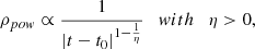 (A.1)
(A.1)around a pole t0 conventionally placed at the end of the bursting period. This distribution is characterized by the burst rate parameter rburst, by Nflares, by the η coefficient, and by τburst, and is called multi-pow;
-
An overlapping set of bursts of activity, with bursts of duration τburst distributed with a log normal distribution. The distribution of flares within each burst follows a power-law distribution (ρpow, reported in Eq. A.1) around a pole t0 conventionally placed at the end of the bursting period. This distribution is characterized by the burst rate parameter rburst, by Nflares, by the η coefficient, and by the parameters of the log-normal distribution (mlog(τ) and σlog(τ)). This distribution is called multi-pow-smooth;
-
A composite model obtained adding a Poissonian process to the multi-loghat fitting function. The event time of a fraction Rfast observed of the events, is extracted at a time distance Δt from an event of the multi-loghat distribution. Δt is extracted with an exponential distribution
 . This distribution is characterized by the burst rate parameter rburst, by Nflares, by the parameters of the log-normal distribution (mlog(τ) and σlog(τ)), and by Rfast observed, τfast. This distribution is called multi-loghat + Poissonian;
 -
A composite model obtained adding a Poissonian process to the multi-pow fitting function. The event time of a fraction Rfast observed of the events is extracted at a time distance Δt from an event of the multi-pow distribution. Δt is extracted with an exponential distribution
 . This distribution is characterized by the burst rate parameter rburst, by Nflares, by the η coefficient, by τburst of the multi-pow distribution, and by Rfast observed, τfast. This distribution is called multi-pow + Poissonian.
The fitting method is explained in Appendix B.
Appendix B: Fitting method
The realization of the fitting distribution is obtained with a Monte Carlo method; it is the simulated distribution of waiting times. It is assumed that the waiting time distribution is the same for all the sources, and that only the observed number of flares can vary from source to source.
For each source, we extract the number of emitted bursts within the observing period, their starting time, and the length. Finally, starting from the observed number of flares for the chosen source, for each flare we extract the burst to which the flare belongs, and the flare starting time within the burst. This last choice corresponds to the assumption that peak flux and duration of each flare does not depend on emission time within a burst. For each source we perform 1000 simulations.
We adopted the binned Cash statistic (Cash 1979) to fit model to the data. There is a chance that a null number of bursts is extracted for a given source. In this case, the simulation cannot reproduce the observed number of flares. So, for each source the probability to observe a given configuration is obtained by the product of the probability that the extracted number of burst is not null ( ) and the usual term discussed in Cash (1979). Thus, we have to add an element for each source to the Cash estimator; this element is
  .
.
Appendix C: Temporal pile-up effect on the waiting times sample
Often authors study crowded periods of activity of blazars trying to resolve single flares with a fitting strategy (see e.g. Abdo et al. 2011; Meyer et al. 2019); a predefined temporal shape for flares is adopted. Often the shape is parametrized, as in equation 7 of Abdo et al. (2010).
In this paper we do not use this method. Only statistically detected peaks with the iSRS method belongs to the studied sample. During crowded periods of activity, the temporal pile-up of flares results in a reduction in the number of detected activity peaks. The pile-up effect was already addressed in Appendix B of Pacciani (2018). Here we compare those findings with the simulated samples.
We simulated flares with a multi-loghat temporal distribution of flaring times. Once the simulated temporal series were obtained for each source, we performed the iSRS procedure to obtain the flaring peak time, luminosity, and duration. The results for the simulated 100 and 300 MeV samples are summarized in figure C.1. We plotted the waiting times versus the minimum among peak fluxes of two consecutive resolved flares (min(Fi, Fi + 1), where Fi and Fi + i are the measured peak fluxes of consecutive flares). To facilitate the comparison, in both the plots the reported flux is evaluated for E> 100 MeV (a power-law index is assumed with index 2.23). The comparison of the two plots reveals that the resolving power is greater for the 100 MeV sample; roughly speaking, the larger statistics allows for an easier separation of close-by flares.
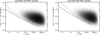 |
Fig. C.1. Distribution of min(Fi, Fi + 1) vs ti + 1 − ti for the simulated 100 and 300 MeV samples (left and right plot, respectively). For the 300 MeV sample the flux was scaled to match the flux for gamma rays above 100 MeV (a power-law flux with photon index of 2.23 is assumed). The solid line is the sensitivity limit for a flare from the bright source 3C 454.3 with FWHM twice the waiting times ti + 1 − ti. The dashed line is the temporal resolving power. |
In the same figure, the sensitivity limit is reported for the detection of a flare with temporal FWHM, which is twice the waiting time, and flux corresponding to min(Fi, Fi + 1). A curve corresponding to the resolving power of consecutive flares is also reported (see Pacciani 2018, for details).
All Tables
Tests for time distribution of flares on sources showing Nflares > 15 in the 100 MeV sample.
Fitted values of the parameters of the multi-loghat, multi-loghat + Poissonian, multi-pow, and multi-pow + Poissonian distributions for the temporal distribution of flares.
Fitting parameters of the multi-loghat model for the temporal distribution of flares.
All Figures
|
Fig. 1. Unbinned light curve (Pacciani 2018) for PKS 1510–08, obtained with Pthr = 1.3 × 10⁻³. Horizontal lines are the statistically relevant clusters. The set of statistically relevant clusters is a tree, and a hierarchy among clusters exists. For each child cluster there is a probability ≤Pthr to be obtained starting from its parent cluster by chance. Vertical bars are the errors on the flux estimate. Background is not subtracted. |
| In the text | |
|
Fig. 2. Distribution of waiting times between gamma-ray flares of FSRQ detected with the iSRS method (100 MeV sample). Left columns: distribution (ρ(log(Δt)) of log(Δt). Right columns: same distribution divided by the bin size; this new distribution is proportional to ρ(log(Δt))e−Δt. The top row reports the distribution for all the sources. The other rows report the distribution of waiting times for sources selected on account of detected flares (from top to bottom): Nflares ≤ 9, 10 ≤ Nflares ≤ 19, Nflares ≥ 20. Solid histograms represent the data, dashed curves the multi-loghat fitting function. The solid grey line in the top row is the composite model obtained adding a Poissonian process to the multi-loghat fitting function. |
| In the text | |
|
Fig. 3. Unbinned light curve (Pacciani 2018) for CTA 102 obtained for E > 100 MeV (see Pacciani 2018, for a detailed explanation), and zoom-ins of the relevant periods. The horizontal segments represent statistically relevant clusters of events obtained with the iSRS procedure. They are described by duration, average photometric flux, and median time (or by starting time). Vertical lines are the error bars on the flux estimate. The set of clusters form a tree called unbinned light curve. Background is not subtracted. |
| In the text | |
|
Fig. 4. Distribution of waiting times for the apparently loudest sources in the sample, and for the whole sample (excluding CTA 102, right bottom plot). Solid histograms represent the data, dashed curves the multi-loghat fitting function evaluated for the whole data sample. For single sources the grey lines represent the multi-loghat fitting function evaluated for each source separately, with parameters reported in Table 3; the fit is performed for Δt > 0.3 d to reduce the contribution of the fast component. |
| In the text | |
|
Fig. 5. Distribution of waiting times for the lensed source S4 0218+35 (observer reference system). Solid histogram represents the data, dashed curve the fitting function. |
| In the text | |
|
Fig. 6. Multi-loghat fit of the waiting times for the 100 MeV sample, and comparison with results reported in Jorstad et al. (2017). Top panel: joint confidence region for rburst and τburst (for the whole 100 MeV sample, excluding CTA 102). The parameters for the minimum of the Cash estimator are reported with a cross. Contours are reported for 90% and 99% confidence levels. The resolved superluminal features ejection rate and fading time observed at 43 GHz (Jorstad et al. 2017) are reported with a diamond symbol (average values). Bottom panel: rburst and τburst (in black) obtained by fitting the multi-loghat distribution to the data of single sources (for the apparently loudest sources in our gamma-ray sample). For comparison, the apparent ejection rate and fading times for each FSRQs reported in Jorstad et al. (2017) are also reported (in grey). |
| In the text | |
|
Fig. 7. Distribution of waiting times for data (grey line), simulated case a (uniformly distributed flares, thin dashed line), and simulated case clct (light crossing time prevails, black continuous line). |
| In the text | |
|
Fig. 8. Statistical distribution of relevant quantities obtained simulating case ccooling. To produce the histograms, the observer line of sight with respect to the jet axis was generated uniformly within a cone of aperture 30°. Top panel: distribution of viewing angles of gamma-ray detected flares. Bottom panel: distribution of Γknotδknot for gamma-ray detected flares. |
| In the text | |
|
Fig. 9. Distribution of relevant parameters for the resolved superluminal features observed at 43 GHz. Left panel: fading time (reported in Table 4 in Jorstad et al. 2017) (log scale). Right panel: Ejection rate (from Table 5 in Jorstad et al. 2017). |
| In the text | |
|
Fig. A.1. Example of burst activity (multi-hat distribution). Each grey rectangle represents a burst of activity. Flares are produced with a uniform distribution inside the bursts of activity. The burst starting time |
| In the text | |
|
Fig. C.1. Distribution of min(Fi, Fi + 1) vs ti + 1 − ti for the simulated 100 and 300 MeV samples (left and right plot, respectively). For the 300 MeV sample the flux was scaled to match the flux for gamma rays above 100 MeV (a power-law flux with photon index of 2.23 is assumed). The solid line is the sensitivity limit for a flare from the bright source 3C 454.3 with FWHM twice the waiting times ti + 1 − ti. The dashed line is the temporal resolving power. |
| In the text | |
Current usage metrics show cumulative count of Article Views (full-text article views including HTML views, PDF and ePub downloads, according to the available data) and Abstracts Views on Vision4Press platform.
Data correspond to usage on the plateform after 2015. The current usage metrics is available 48-96 hours after online publication and is updated daily on week days.
Initial download of the metrics may take a while.