| Issue |
A&A
Volume 689, September 2024
|
|
|---|---|---|
| Article Number | A56 | |
| Number of page(s) | 12 | |
| Section | Extragalactic astronomy | |
| DOI | https://doi.org/10.1051/0004-6361/202449726 | |
| Published online | 30 August 2024 | |
The flaring activity of blazar AO 0235+164 in 2021
1
Instituto de Astrofísica de Andalucía, CSIC, Glorieta de la Astronomía s/n, 18080 Granada, Spain
2
Institute for Astrophysical Research, Boston University, 725 Commonwealth Avenue, Boston, MA 02215, United States
3
Department of Astronomy, University of Geneva, ch. d’Ecogia 16, 1290 Versoix, Switzerland
4
Department of Physics, University of Crete, 71003 Heraklion, Greece
5
Institute of Astrophysics, Foundation for Research and Technology – Hellas, Voutes, 70013 Heraklion, Greece
6
Institut de Radioastronomie Millimétrique, Avenida Divina Pastora 7, Local 20, 18012 Granada, Spain
7
INAF – Istituto di Radioastronomia, Via Gobetti 101, 40129 Bologna, Italy
8
INAF Osservatorio Astronomico di Brera, Via E. Bianchi 46, 23807 Merate (LC), Italy
9
Saint Petersburg State University, 7/9 Universitetskaya nab., St. Petersburg 199034, Russia
10
Center for Astrophysics – Harvard & Smithsonian, 60 Garden Street, Cambridge, MA 02138, USA
Received:
25
February
2024
Accepted:
15
May
2024
Abstract
Context. The blazar AO 0235+164, located at redshift z = 0.94, has displayed interesting and repeating flaring activity in the past, with recent episodes in 2008 and 2015. In 2020, the source brightened again, starting a new flaring episode that peaked in 2021.
Aims. We study the origin and properties of the 2021 flare in relation to previous studies and the historical behavior of the source, in particular the 2008 and 2015 flaring episodes.
Methods.We analyzed the multiwavelength photo-polarimetric evolution of the source. From Very Long Baseline Array images, we derived the kinematic parameters of new components associated with the 2021 flare. We used this information to constrain a model for the spectral energy distribution of the emission during the flaring period. We propose an analytical geometric model to test whether the observed wobbling of the jet is consistent with precession.
Results. We report the appearance of two new components that are ejected in a different direction than previously, confirming the wobbling of the jet. We find that the direction of ejection is consistent with that of a precessing jet. Our derived period agrees with the values commonly found in the literature. Modeling of the spectral energy distribution further confirms that the differences between flares can be attributed to geometrical effects.
Key words: accretion / accretion disks / astroparticle physics / polarization / radiation mechanisms: general / relativistic processes / galaxies: jets
Corresponding author; This email address is being protected from spambots. You need JavaScript enabled to view it. .
© The Authors 2024
 Open Access article, published by EDP Sciences, under the terms of the Creative Commons Attribution License (https://creativecommons.org/licenses/by/4.0), which permits unrestricted use, distribution, and reproduction in any medium, provided the original work is properly cited.
This article is published in open access under the Subscribe to Open model. This email address is being protected from spambots. You need JavaScript enabled to view it. to support open access publication.
1. Introduction
Blazars, a type of active galactic nucleus (AGN), are amongst the most energetic objects in the Universe. They are generally accepted to consist of a supermassive black hole (BH) surrounded by an accretion disk and usually a dusty torus (DT), with symmetrical jets of matter emanating from the vicinity of the BH that can extend far beyond the size of its host galaxy. The exact mechanisms by which high-energy emission from blazars is generated are not well understood, and questions remain about the exact mechanisms by which plasma in the jet is collimated and accelerated to speeds close to that of light, as well about the particle composition of the jet and the location and cause of the observed variability and γ-ray emission.
AO 0235+164 is a BL Lacertae-type blazar located at redshift z = 0.94 (Cohen et al. 1987). It exhibits strong variability across the entire spectrum, and has repeatedly displayed high-amplitude flaring behavior in recent years. In particular, episodes in 2008 (Agudo et al. 2011) and 2015 (Escudero et al. 2024), which received extensive multiwavelength (MWL) coverage, displayed significant similarities: significant correlations and short delays between emission at different bands, X-ray spectrum features beyond the absorption expected from our Galaxy (Madejski et al. 1996), and the association of flaring episodes with the appearance of superluminal components in very long baseline interferometry (VLBI) images of the source, among others (Agudo et al. 2011; Escudero et al. 2024).
The similar time span between these episodes, together with older studies of the source (Raiteri et al. 2005) that reported flares in previous decades (1992, 1998), hints at a pseudo-periodic behavior with a characteristic timescale of 6–8 years (Otero-Santos et al. 2023). A similar timescale was suggested by Ostorero et al. 2004, who explained the nearly periodic long-term variability at lower frequencies with a helical model of the jet that precisely matched most of the flares at 8 GHz between 1975–2000 with a period of almost 6 years. The predicted flare in 2004, however, failed to occur, although a period of stronger variability started that peaked in early 2006 and culminated in the historic peak of October 2008. So far, all attempts at uncovering a significant and clear periodicity in the emission of AO 0235+164 have failed: the emission, albeit repeating and presenting striking similarities each time, is not periodic (i.e., there is no precise delay or close resemblance between different periods). On the other hand, the flares are a recurrent phenomenon, and the existence of a characteristic timescale for the system related to the apparent delay of 6–8 years between flares cannot be discarded. In this regard, there might be other hints of periodic or pseudo-periodic behavior in this source.
We present data from the most recent flare of AO 0235+164, which occurred in 2021, extending the dataset from Escudero et al. (2024) by 4 years, from 2019 to 2023. The new episode confirms the relationship between flares in the different spectral ranges, the appearance of superluminal components in VLBI images, and the changing direction of the propagation of these components. The timing of this new flare and its detailed characteristics, which we present here, further strengthen the hypothesis of a pseudo-periodic behavior.
For this work we used a standard flat ΛCDM cold dark matter cosmological model with Hubble constant H0 = 67.66 km/Mpc, as given by Planck Collaboration VI (2020).
2. Observations
The new dataset presented in this study extends in time by about three years the one in Escudero et al. (2024), and includes 7mm (43 GHz) Very Long Baseline Array (VLBA) images from the Boston University blazar monitoring program (VLBA-BU-BLAZAR and BEAM-ME programs), reduced both for total flux density and polarization using AIPS (see Weaver et al. 2022); single-dish photo-polarimetric data at 1 mm and 3 mm from the POLAMI1 program at the IRAM 30m Telescope (Agudo et al. 2017a; Thum et al. 2017; Agudo et al. 2017b); photometric data at 1mm and 0.8μm from the Submillimeter Array (SMA), including photo-polarimetric data at 1mm from the SMAPOL program (see Appendix A for details); 8mm observations from the Metsähovi Radio Observatory, and optical data from the Calar Alto (2.2 m Telescope) under the MAPCAT program and from the Perkins Telescope Observatory (1.8 m Telescope). Gamma-ray data in the 0.1–200 GeV range come from the Fermi/Large Area Telescope. The historical light curve shown in Figure 1 also contains previously published optical data from the Crimea Observatory AZT-8 (0.7 m Telescope) and the St. Petersburg State University LX-200 (0.4 m Telescope), as well as ultraviolet data from the Swift/UVOT instrument, X-ray data in the 2.4–10 keV range from the RXTE satellite, and in the 0.2–10 keV energy range from Swift/XRT (see Escudero et al. 2024 for details).
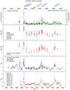 |
Fig. 1. Historical light curves of AO 0235+164 at different wavelengths. The first four vertical lines mark the epochs analyzed in Escudero et al. (2024); the last one corresponds to the epoch analyzed in Sect. 3.6. |
We followed the procedure described in Blinov & Pavlidou (2019) to overcome the ±180° polarization angle ambiguity in our R-band measurements, minimizing the difference between successive measurements while also taking into account their uncertainty. We also shifted clusters of close observations by an integer multiple of 180° to match the angle reported at 3mm, enabling a visual comparison of the joint evolution of the optical and millimeter range polarization angles, while maintaining the short time evolution intact. Data from the infrared to the ultraviolet bands were corrected following the prescription by Raiteri et al. (2005) and the updated values by Ackermann et al. (2012). This correction accounts for the local Galactic extinction at z = 0 and the intervening galaxy ELISA at z = 0.524, as well as for ELISA’s contribution to the observed emission. Details about the correction to the X-ray present in the historical light curve are available in Escudero et al. (2024).
3. Analysis and results
3.1. Multiwavelength flux and polarization behavior
In Figure 1 we present the MWL light curves consisting of our compiled data in the millimeter, optical, and high-energy ranges from 2008 to 2023. This period includes the three recent flaring episodes of the source in 2008, 2015 and 2021. A detailed view into the last of these flaring episodes can be found in Figure 2. During the flare, emission at all wavelengths experienced an increase, from millimeter-wave to high-energy γ-rays, as happened in previous flaring episodes. Compared to previous flares of the source, the 2021 flare was weaker, following a trend that started with the 2015 episode. In agreement with past episodes, the light curve during the 2021 flare shows a multi-peak structure, with sharper variability at higher energies.
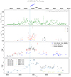 |
Fig. 2. Zoomed-in view of the flux evolution of AO 0235+164 at different wavelengths in 2019–2923. The vertical line corresponds to the last marked date in Fig. 1. |
The evolution of both the linear polarization degree and the polarization angle at all wavelengths are shown in Figures 3 and 4, respectively. The polarization degree also increased during the episode, from pL, R = 10.0 ± 6.0% and pL, 3mm = 3.0 ± 1.4% in the time spanned from 2018 to 2019 to pL, R = 12.5 ± 6.3% and pL, 3mm = 3.7 ± 2.0% from 2019 to 2023, although this increase was not as dramatic as in the previous flaring episodes (Escudero et al. 2024). In contrast to the 2015 episode, the polarization angle at 3mm remained more stable, with no clear rotations apparent in the available data.
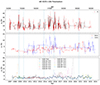 |
Fig. 3. Historical evolution of the polarization degree of AO 0235+164. A Bayesian block representation is shown superimposed for R at 99.9% confidence and for 1mm and 3mm at 90% confidence. Vertical lines corresponds to the dates marked in Fig. 1. |
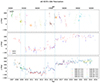 |
Fig. 4. Historical evolution of the polarization angle of AO 0235+164. Vertical lines correspond to the dates marked in Fig. 1. All points in the first panel correspond to the R band; the different colors denote the clusters that were shifted by n × 180° to follow the evolution of the polarization angle at 3mm, as discussed in Sect. 2. |
3.2. VLBA imaging
We analyzed a total of 49 new VLBA 7mm (43 GHz) images of AO 0235+164, extending the dataset presented in Escudero et al. (2024) by about 4 years. In our new VLBI images, the most recent flare is accompanied by the ejection of newly emerged components B8 and B9, as can be seen in Figure 5 for some selected epochs. These components move away from the compact, stationary region present at all epochs known as the “core”. As in our previous studies, these components were obtained by fitting the reduced VLBA total flux maps to circular Gaussian components in the (u, v) plane using Difmap. After model fitting of the most prominent jet features, we cross-identified them along the different observing epochs. This was done for all new 49 observing epochs. Their resulting flux and polarization evolution is shown in Figures 3 and 4, together with that of the core region (labeled as component A0) and the total integrated emission from the source at 7mm.
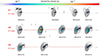 |
Fig. 5. Selected epochs illustrating the evolution of the last three identified components, B7, B8, and B9. The figure shows the total intensity (contours), polarized flux intensity (color sale), and polarization direction (black line segments). The horizontal black line marks the position of the core, A0. The red line in each row is a linear fit to the knot position, present for all except B7 due to its low flux. For each row, the spacing between plots is proportional to the elapsed time, with the total time indicated in parentheses. The full temporal evolution is available as an online movie. |
The connection between the MWL flare and the ejection of superluminal components in VLBA images at 7mm is confirmed here for the 2021 flare, as was also found for the 2006–2008 flare(s), which was accompanied by the appearances of components B1 and B2, and for the 2015 flare, when components B5, B6, and B7 were ejected. We observe that the increase in brightness of the core (A0) begins almost a year before the new B8 component can be differentiated, although the polarization angle is already aligned with the future direction of B8. This alignment is maintained for most of the lifetime of the component, except for short rotations just after its ejection. This behavior was also reported previously for the superluminal components associated with the 2008 and 2015 flares, and also for components B3 and B4 during the quiescent period in between those two flares (Escudero et al. 2024).
Remarkably, the direction of propagation of these new components is very different from that of traveling components identified previously in AO 0235+164 with the VLBA at 7mm. In fact, it has been the case for AO 0235+164 that the direction of ejection has consistently changed from one episode to the next: B1 (111 ± 3°), B2 (−72 ± 16°), B3 (−73 ± 10°), B4 (153 ± 21°), B5 (29 ± 4°), B6 (40 ± 10°), B7 (70 ± 10°), B8 (147 ± 8°), and B9 (144 ± 8°). The new flare and its associated traveling components confirm the wobbling of the jet and its narrow viewing angle. A very low viewing angle of the jet is necessary for any reasonably small change in its direction to produce such radical changes in the direction on the sky of propagation of the superluminal components.
3.3. Kinematic parameters of the VLBI jet components
We computed the kinematic parameters of the new B8 component following the procedure described in Weaver et al. (2022), as was done in Escudero et al. (2024) for B1 to B6. The procedure involved tracing the identified features in the VLBA images across all new epochs and fitting their positions to a linear function to obtain their speed (vr) and time of ejection (t0), as well as fitting their fluxes to a decaying exponential to obtain the timescale of variability (tvar). This allowed us to compute their Doppler factor δ and apparent speeds βapp (Jorstad et al. 2005; Casadio et al. 2015). From these, the corresponding bulk Lorentz factors, Γ, and viewing angles, Θ, could be computed using the usual expressions. As was the case for B7 during the previous flare, the kinematic parameters of B9 could not be correctly estimated due to the low number of observations, and only the time of ejection could be computed for B7 and B9. The fits to the position and flux of B8 can be found in Figure 6. For B8, we obtained a time of ejection t0 = 2020.0 ± 0.2 year, Doppler factor δvar = 25.5 ± 1.5, apparent speed βapp = 6.7 ± 1.0, bulk Lorentz factor Γ = 13.6 ± 1.7 and viewing angle Θ = 1.1 ± 0.2°. These results are in agreement with those found in Escudero et al. (2024). The Doppler factor of B8, the main ejected component responsible for the 2021 flare, is much lower than that of B2 for the 2008 flare (δ = 67.8 ± 3.6) and B5 for the 2015 flare (δ = 39.8 ± 2), explaining the relatively diminished luminosity of each flare as a consequence of weaker Doppler boosting.
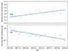 |
Fig. 6. Observed distance from the core (top) and flux density (bottom) for the newly identified component, B8, together with the linear weighted fit to the flux knot position and the logarithmic fit to the knot flux used in the computation of the kinematic parameters. |
3.4. Change in jet direction
To try to explain the observed wobbling of the jet, we used the derived times of ejection of the superluminal components and their direction of propagation to test for signs of a precessing jet by fitting to an analytical model for the angle of propagation. If we assume that the ejection happens at approximately constant distance from the base of the jet, this location, when projected in the plane of the sky, must trace an ellipse for which the eccentric anomaly E is given by the precessed angle, E = ωt. The eccentricity of this ellipse will be given by the angle between the axis of precession and the observer. In arbitrary units, the semi-axes of this ellipse can be taken to be a = 1 and b = cos φ. In the plane of the sky, the center of this ellipse will be displaced with respect to the basis of the jet by a distance d sin φ, and the major semi-axis will form an arbitrary angle, ψ, with regard to the x-axis. The polar coordinate of this region orbiting along the ellipse with respect to the basis of the jet is the observed angle of propagation of the superluminal component. If the angle between the precession axis and the observer is high enough compared to the tilt of the jet with regard to the precession axis, the jet will have a definite direction in the sky, and all components will be emitted in the span of some arc. When the jet is narrowly pointing toward us, even for small precession angles, the superluminal components will appear to propagate in all directions. This would be the case for AO 0235+164.
Figure 7 shows the result of simultaneously fitting (t0, cos θ) and (t0, sin θ), where θ is the propagation angle of a component. This fit was preferred to directly fitting the angle θ because it removes any ambiguity in the position angle. The uncertainties in the parameters were computed using a Monte Carlo approach. Only components B2 to B8 were used for the fit, on the basis of selecting only those with a significant number of epochs to compensate for the high uncertainties in the positions of the fitted Gaussian features mentioned in Sect. 3.2. We examined the impact of considering all components in the fit and concluded that the optimal fit values were comparable, despite a significant increase in the model uncertainties. The resulting best-fit model has a period of T = (6.0 ± 0.1) years, which is within the range of periods proposed in the literature. The obtained eccentricity of the ellipse gives an angle of ϕ = 0.11° for the hypothetical precession axis with regard to the observer, although this value is not well constrained by our fit. Because of the low number of points and the significant uncertainties in the times of ejection of jet features, usual fit statistics such as the p-value are not suitable to reaffirm or reject our hypothesis, and therefore do not allow us to claim precession in AO 0235+164. Nevertheless, we find it interesting to examine Figures 7 and 8, where it can be seen that most of the points fall inside the 3σ region when accounting for their uncertainties. We propose that the model might be used to affirm or discard the hypothesis of precession when more data become available in subsequent decades. We also emphasize that the value for the period found in this analysis, derived from the propagation angle of superluminal components, is independent of the periods suggested in the literature (Otero-Santos et al. 2023; Raiteri et al. 2005; Ostorero et al. 2004), which are derived from analysis of variations in the light curves. They nevertheless agree within their uncertainties. The small value obtained for the possible precession axis relative to the line of sight, together with the viewing angles obtained in the kinematic analysis (Sect. 3.3), is also in agreement with the observed behavior of the jet, which ejects components in completely different directions.
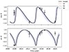 |
Fig. 7. Simultaneous fit to the sine and cosine of the average position angle, θ, of the identified VLBI jet features as a function of their computed time of ejection. Most of the points lie within the 3σ model uncertainty region. The simultaneous fit avoids the ±180 uncertainty in the position angle. The corresponding plot for the position angle, θ, can be found in Fig. 8. |
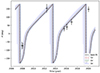 |
Fig. 8. Observed ejection angles of the identified VLBI components B2-B8 with respect to their computed time of ejection, together with the best-fit model. The shaded areas represent the 1σ (68.27%), 2σ (95.45%), and 3σ (99.73%) uncertainties of the model. |
3.5. Correlations across the spectrum
We computed the correlations between the light curves at different wavelengths using MUTIS2. We used the normalized discrete correlation function (DCF) proposed by Welsh (1999), which applies normalization and binning, making it suitable for our irregularly sampled signals. A uniform bin size of 20days was used, a value that was chosen to allow for enough bin statistics without smoothing the correlations too much. To validate our choice, the same results were derived using binning sizes from 10 days to 30 days, confirming the consistency of our results. The significance of the correlations was estimated using a Monte Carlo approach, generating N = 2000 synthetic light curves for each signal. Randomization of the Fourier transform was used for millimeter wavelengths, generating light curves with similar statistical properties and power-spectrum density (PSD). For optical and γ-ray data we modeled the signals as Orstein-Uhlenbeck stochastic processes (Tavecchio et al. 2020), which better reproduces the qualitative shape of these signals. The uncertainties of the correlations were estimated using the uncertainties of the signals, again with a Monte Carlo approach. We find high and significant correlations between emission from all bands except X-rays (Fig. 9), for which correlation was generally lower and found only at 2σ with some bands. This is in agreement with our previous results (Escudero et al. 2024) that found decreased correlation for the X-ray band and attributed it to a different emission mechanism located at a different region. Nonetheless, the achieved significance of those correlations involving X-rays are generally higher than those previously found, thanks to the improved dataset. This is especially the case for the correlation between X-rays and 1mm, where no significant correlation was previously found. This decreased correlation for the X-ray is also expected from the spectral energy distribution modeling presented in Sect. 3.6 and that of Escudero et al. (2024), where the bulk Compton emission dominates the X-rays in its high state, while in its low state it is dominated by the same region responsible for emission in other bands. Regarding correlations restricted only to the last episode (2019–2023), the new flare is too weak and data too sparse to produce any meaningful correlations, which are dominated by noise, so they have been omitted here.
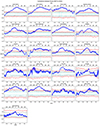 |
Fig. 9. Correlations between fluxes at all wavelengths. Horizontal lines represent the 1σ, 2σ, and 3σ significance levels and were computed using a Monte Carlo approach with N = 2000 synthetic light curves. We find clear and significant (> 3σ) correlations near zero between all bands except for the X-ray. |
Analysis of the PSD of the signals was performed using the Lomb-Scargle periodogram (Lomb 1976; Scargle 1982), suitable for our unevenly sampled light curves. The resulting power spectra locate the peak frequencies of the 1mm, 3mm, 7mm, 8mm, and R-band light curves at equivalent timescales of 5.7, 5.4, 5.1, 4.2, and 6.8 years, respectively (Fig. 10). Computed false-alarm probabilities are close to zero in all cases (≪0.1%). The interpretation of this probability is subtle (VanderPlas 2018), but instead hints at a low probability of a purely stochastic process, since it represents the probability of a purely noise signal producing a peak higher than ours. The derived timescales agree with those suggested in the literature (Otero-Santos et al. 2023; Raiteri et al. 2005; Ostorero et al. 2004) and with the one independently obtained in Sect. 3.4.
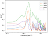 |
Fig. 10. Normalized PSD computed using the Lomb-Scargle periodogram for the 1mm, 3mm, 7mm, 8mm, and R light curves, showing peak frequencies corresponding to characteristic timescales of 5.7, 5.4, 5.1, 4.2, and 6.8 years, respectively. These timescales are mostly in agreement with the 5–8 year timescale found in previous works. The false alarm probability in all cases is close to zero (≪0.1%), meaning that there is a very low probability that such a peak would be caused by a pure noise signal. |
3.6. Spectral energy distribution
Unlike for previous flares, no Swift XRT or UVOT data are available during the flaring period in 2021. The night with the broadest MWL coverage (MJD 59113, October 20, 2020) was selected to perform a spectral energy model of the source.
We modeled the emission using the JetSeT framework (Tramacere 2020; Tramacere et al. 2011, 2009) using both a single-zone synchrotron self-Compton (SSC) scenario and an SSC plus external Compton (EC) scenario. The common physical setup consists of a spherical emitting region formed by a population of relativistic electrons of radius R at a distance RH from the central BH that moves at a small angle, θ, to the line of sight with a bulk Lorentz factor, Γ. Synchrotron radiation is emitted through interaction of the relativistic electrons with the jet magnetic field, B. These same synchrotron photons and electrons interact by inverse Compton scattering to produce high-energy photons (SSC). In the EC scenario, additional radiation is produced from inverse Compton scattering of photons coming from a disk torus (disk) and broad line region (BLR) surrounding the BH. The electron energy distribution is assumed to be well described by a power law with a cutoff (PLC):
 (1)
(1)
where p is the spectral index and γ is the electron Lorentz factor. A broken power law was also attempted, but the resulting fit was systematically worse, consistent with the results of Escudero et al. (2024), and therefore we only show the model with the PLC distribution.
In the single-zone SSC scenario, it was found that the region of emission was best described as having a radius  , situated at a distance RH = 9.3 × 1019cm with a bulk Lorentz factor
  , and a viewing angle of
  , while the electron distribution was best modeled as having a spectral index
  , and minimum and maximum Lorentz factors of
  ,
,  , and a cutoff of
  . The best-fit value for the magnetic field was
  . All values reported are best-fit values, with 1σ asymmetric errors computed using Markov chain Monte Carlo approach. The result has been represented in Fig. 11. The obtained parameters are in agreement with those obtained by Escudero et al. (2024), and the resulting bulk Lorentz factor, viewing angle, and Doppler factor (δ = 25) agree precisely with those obtained in the kinematic analysis of section 3.3 within their uncertainties.
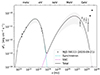 |
Fig. 11. Spectral energy distribution from September 21, 2023, together with the best fit of the one-zone SSC model discussed in Section 3.6. The gray area represents the 3σ uncertainty region. The downward pointing triangles represent upper limits. |
In the EC scenario, the disk, DT, and BLR parameters were frozen. The disk was assumed to have luminosity LDisk = 5 × 1045 erg s−1, accretion efficiency η = 0.08, and inner and outer radii RDisk, in = 3Rs and RDisk,out = 300Rs, respectively. The DT temperature was fixed to TDT = 830K, its radius determined by the phenomenological relation  (Cleary et al. 2007), with reprocessing factor τDT = 0.1. The BLR was modeled as a thin spherical shell with an internal radius as provided by the phenomenological relation
  (Kaspi et al. 2007) and its outer radius was assumed to be RBLR,out = 1.1RBLR,in, with a coverage factor τBLR = 0.1. The mass of the BH was set to MBH = 5 × 10⁸ M⊙.
Two alternative SSC+EC models were produced, one allowing Γ and θ to vary freely and the other fixing them to the values obtained from the kinematic analysis. In the former case, the emitting region was best described by best-fit values  ,
,  ,
,  ,
,  ,
,  ,
,  ,
,  , and
, and  . In the latter, fixing Γ = 13.6 and θ = 0.9°, we obtained
  ,
,  ,
,  ,
,  ,
,  , and
, and  . The higher bulk Lorentz factor in the first cause with respect to that measured at the VLBI case might be attributed to deceleration. The results have been represented in Figs. 12 and 13. In any case, for all models the resulting Doppler factors are lower than that obtained for the flaring epochs in the 2008 (δ = 37) and 2015 (δ = 32) episodes (Escudero et al. 2024), which consistently explains the lower apparent luminosities of the successive flares as caused, at least partially, by relativistic effects.
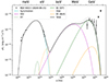 |
Fig. 12. Spectral energy distribution from September 21, 2023, together with the best fit of the SSC+EC model with freely varying Γ and θ as discussed in Section 3.6. The gray area represents the 3σ uncertainty region. The downward pointing triangles represent upper limits. |
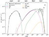 |
Fig. 13. Spectral energy distribution from September 21, 2023, together with the best fit of the SSC+EC model with fixed Γ and θ as discussed in Section 3.6. The gray area represents the 3σ uncertainty region. The downward pointing triangles represent upper limits. |
4. Discussion and conclusions
We have presented new and updated data from the blazar AO 0235+165, extending previous works to cover its most recent flaring episode, which peaked in 2021.
The new flare is again associated with the appearance of two new components in 7mm VLBA images, B8 and B9. The behavior of B9 and B8 is compatible with that of trailing components (Agudo et al. 2001), as was the case with B6 and B5 during the 2015 episode. This can be interpreted in the context of a shock-in-jet model, in agreement with the alignment of the polarization angle in the direction of the jet axis that begins during the core re-brightening phase (Fig. 5). The two newly identified components, B8 and B9, propagate in a different direction compared to previous components, confirming the wobbling of the jet.
We have proposed a purely geometrical model that aims to explain the observed changes in the direction of the ejection of the VLBI components as the result of a precessing jet. We have found that the observed position angles and calculated times of ejection are mostly compatible with a jet precessing with a period of 6 years. This value is independently obtained but compatible with those found in the existing literature. Although precession is a strictly periodic phenomenon and no exact periodicity is found in the MWL light curves of AO 0235+164, it is important to keep in mind that the model in Sect. 3.4 relates only to the position angle of the ejected components. However, the periodicity found in this model must indeed have an origin that could justify the timescale of variability – not periodicity – of 6 − 8 years found in the light curves in previous works (Raiteri et al. 2005; Otero-Santos et al. 2023) and in Sect. 3.5. The absence of a strict periodicity in the flux evolution of the source is to be expected due to the fact that jet emission is a complex process that can be affected by many factors (jet angle, speed, magnetic field, matter accretion, and available energy, to name only a few) and is inherently stochastic. However, the possible origins of wobbling, or jet precession, are more restricted, the most common causes being a binary system (Abraham 2018) or an off-axis accretion disk (Lense-Thirring effect), and this exact periodicity can be distortedly reflected in light curves. A precessing jet with a periodicity of around ∼6 years could explain the pseudo-periodic timescale found in the light curves in previous works.
Modeling of the spectral energy distribution reveals that the emission process is similar to that of previous epochs, both flaring and quiescent (Escudero et al. 2024), with the difference in the Doppler factor explaining at least partially the flux variability. This is the case for all bands but cannot be confirmed in X-rays due to the absence of data during the 2021 flaring episode. However, previous works found that emission in X-rays was caused at least partially by different, uncorrelated mechanisms involving a different emitting region, and that this region was responsible for the bulk of emission when the X-ray emission was in its high state (Ackermann et al. 2012; Escudero et al. 2024). Therefore, more complex models are necessary to fully explain the MWL emission. Moreover, even the aforementioned models fail to include hadronic processes despite increasing evidence of neutrino emission in blazars (IceCube Collaboration 2018).
The re-brightening of the core suggests the existence of a standing shock, with the ejected components that accompany each flaring episode interpreted as trailing components (Agudo et al. 2001). Such stationary shocks can be explained by bends in the jet, which are expected in wobbling jet scenarios, although such bends need not be caused by rotations of the jet nozzle: they can also be the result of dynamical processes. In addition, stationary shocks can be explained by the interaction of the jet with the external medium (Gómez et al. 1997). In any case, the recurrence of the flaring episodes, the wobbling of the jet, and the modeling of the spectral energy distribution suggest the existence of a characteristic timescale of a periodic and geometric origin that must be well characterized to achieve a full understanding of the mechanisms of AO 0235+164 emission.
Data availability
Movie associated with Fig. 5 is available at https://www.aanda.org
MUltiwavelength TIme Series. A Python package for the analysis of correlations of light curves and their statistical significance. https://github.com/IAA-CSIC/MUTIS
Acknowledgments
The IAA-CSIC team acknowledges financial support from the Spanish “Ministerio de Ciencia e Innovación” (MCIN/AEI/ 10.13039/501100011033) through the Center of Excellence Severo Ochoa award for the Instituto de Astrofísica de Andalucía-CSIC (CEX2021-001131-S), and through grants PID2019-107847RB-C44 and PID2022-139117NB-C44. This research has made use of the NASA/IPAC Extragalactic Database (NED), which is operated by the Jet Propulsion Laboratory, California Institute of Technology, under contract with the National Aeronautics and Space Administration. IRAM is supported by INSU/CNRS (France), MPG (Germany) and IGN (Spain). The VLBA is an instrument of the National Radio Astronomy Observatory, USA. The National Radio Astronomy Observatory is a facility of the National Science Foundation operated under cooperative agreement by Associated Universities, Inc. This study was based (in part) on observations conducted using the 1.8 m Perkins Telescope Observatory (PTO) in Arizona (USA), which is owned and operated by Boston University. The BU group was supported in part by U.S. National Science Foundation grant AST-2108622, and NASA Fermi GI grants 80NSSC23K1507, 80NSSC22K1571 and 80NSSC23K1508. The Submillimeter Array is a joint project between the Smithsonian Astrophysical Observatory and the Academia Sinica Institute of Astronomy and Astrophysics and is funded by the Smithsonian Institution and the Academia Sinica. We recognize that Maunakea is a culturally important site for the indigenous Hawaiian people; we are privileged to study the cosmos from its summit.
References
- Abraham, Z. 2018, Nat. Astron., 2, 443 [NASA ADS] [CrossRef] [Google Scholar]
- Ackermann, M., Ajello, M., Ballet, J., et al. 2012, ApJ, 751, 159 [NASA ADS] [CrossRef] [Google Scholar]
- Agudo, I., Gómez, J.-L., Martí, J.-M., et al. 2001, ApJ, 549, L183 [Google Scholar]
- Agudo, I., Marscher, A. P., Jorstad, S. G., et al. 2011, ApJ, 735, L10 [NASA ADS] [CrossRef] [Google Scholar]
- Agudo, I., Thum, C., Molina, S. N., et al. 2017a, MNRAS, 474, 1427 [Google Scholar]
- Agudo, I., Thum, C., Ramakrishnan, V., et al. 2017b, MNRAS, 473, 1850 [Google Scholar]
- Baring, M. G., Böttcher, M., & Summerlin, E. J. 2017, MNRAS, 464, 4875 [CrossRef] [Google Scholar]
- Blinov, D., & Pavlidou, V. 2019, Galaxies, 7 [Google Scholar]
- Casadio, C., Gómez, J. L., Jorstad, S. G., et al. 2015, ApJ, 813, 51 [Google Scholar]
- Cleary, K., Lawrence, C. R., Marshall, J. A., Hao, L., & Meier, D. 2007, ApJ, 660, 117 [CrossRef] [Google Scholar]
- Cohen, R. D., Smith, H. E., Junkkarinen, V. T., & Burbidge, E. M. 1987, ApJ, 318, 577 [NASA ADS] [CrossRef] [Google Scholar]
- Escudero, J., Agudo, I., Tramacere, A., et al. 2024, A&A, 682, A100 [NASA ADS] [CrossRef] [EDP Sciences] [Google Scholar]
- Gómez, J. L., Martí, J. M., Marscher, A. P., Ibáñez, J. M., & Alberdi, A. 1997, ApJ, 482, L33 [Google Scholar]
- Ho, P. T. P., Moran, J. M., & Lo, K. Y. 2004, ApJ, 616, L1 [Google Scholar]
- IceCube Collaboration (Aartsen, M. G., et al.) 2018, Science, 361, eaat1378 [NASA ADS] [Google Scholar]
- Jorstad, S. G., Marscher, A. P., Lister, M. L., et al. 2005, AJ, 130, 1418 [Google Scholar]
- Kaspi, S., Brandt, W. N., Maoz, D., et al. 2007, ApJ, 659, 997 [NASA ADS] [CrossRef] [Google Scholar]
- Lomb, N. R. 1976, Ap&SS, 39, 447 [Google Scholar]
- Madejski, G., Takahashi, T., Tashiro, M., et al. 1996, ApJ, 459, 156 [NASA ADS] [CrossRef] [Google Scholar]
- Ostorero, L., Villata, M., & Raiteri, C. M. 2004, A&A, 419, 913 [NASA ADS] [CrossRef] [EDP Sciences] [Google Scholar]
- Otero-Santos, J., Peñil, P., Acosta-Pulido, J. A., et al. 2023, MNRAS, 518, 5788 [Google Scholar]
- Planck Collaboration VI. 2020, A&A, 641, A6 [NASA ADS] [CrossRef] [EDP Sciences] [Google Scholar]
- Primiani, R. A., Young, K. H., Young, A., et al. 2016, J. Astron. Instrum., 5, 1641006 [NASA ADS] [CrossRef] [Google Scholar]
- Raiteri, C. M., Villata, M., Ibrahimov, M. A., et al. 2005, A&A, 438, 39 [NASA ADS] [CrossRef] [EDP Sciences] [Google Scholar]
- Scargle, J. D. 1982, ApJ, 263, 835 [Google Scholar]
- Shaw, R. A., Payne, H. E., & Hayes, J. J. E. 1995, ASP Conf. Ser., 77, 433 [NASA ADS] [Google Scholar]
- Tavecchio, F., Bonnoli, G., & Galanti, G. 2020, MNRAS, 497, 1294 [NASA ADS] [CrossRef] [Google Scholar]
- Thum, C., Agudo, I., Molina, S. N., et al. 2017, MNRAS, 473, 2506 [Google Scholar]
- Tramacere, A. 2020, JetSeT: Numerical modeling and SED fitting tool for relativistic jets, Astrophysics Source Code Library [record ascl:2009.001] [Google Scholar]
- Tramacere, A., Giommi, P., Perri, M., Verrecchia, F., & Tosti, G. 2009, A&A, 501, 879 [NASA ADS] [CrossRef] [EDP Sciences] [Google Scholar]
- Tramacere, A., Massaro, E., & Taylor, A. M. 2011, ApJ, 739, 66 [Google Scholar]
- VanderPlas, J. T. 2018, ApJS, 236, 16 [Google Scholar]
- Weaver, Z. R., Jorstad, S. G., Marscher, A. P., et al. 2022, ApJS, 260, 12 [NASA ADS] [CrossRef] [Google Scholar]
- Welsh, W. F. 1999, PASP, 111, 1347 [Google Scholar]
Appendix A: SMAPOL observations
The SMA (Ho et al. 2004) was used to obtain polarimetric millimeter radio measurements at 1.3 mm (230 GHz) within the framework of the SMAPOL (SMA Monitoring of AGNs with POLarization) program. SMAPOL follows the polarization evolution of forty γ-ray bright blazars, including AO 0235+164, on a bi-weekly cadence, as well as other sources in a target-of-opportunity mode. The observations reported here were conducted between July 2022 and December 2023.
The SMA observations use two orthogonally polarized receivers, tuned to the same frequency range in full polarization mode, and use the SWARM correlator (Primiani et al. 2016). These receivers are inherently linearly polarized but are converted to circular using the quarter-wave plates of the SMA polarimeter (Primiani et al. 2016). The lower sideband (LSB) and upper sideband (USB) covered 209-221 and 229– 241GHz, respectively. Each sideband was divided into six chunks, with a bandwidth of 2GHz, and a fixed channel width of 140kHz. The SMA data were calibrated with the MIR software package 3. Instrumental polarization leakage was calibrated independently for USB and LSB using the MIRIAD task gpcal (Shaw et al. 1995) and removed from the data. The polarized intensity, position angle, and polarization percentage were derived from the Stokes I, Q, and U visibilities.
AO 0235+164 was observed 14 times within the above period on June 1, 4, and 16 with integration times between 2.4 and 15 minutes. The total flux density, linear polarization degree and polarization angle results are given in the table attached. MWC 349 A, Callisto, Uranus, Neptune, and Ceres were used for the total flux calibration according to their visibility, and the calibrator 3C 286, which has a high linear polarization degree and stable polarization angle, was observed regularly as a cross-check of the polarization calibration.
All Figures
|
Fig. 1. Historical light curves of AO 0235+164 at different wavelengths. The first four vertical lines mark the epochs analyzed in Escudero et al. (2024); the last one corresponds to the epoch analyzed in Sect. 3.6. |
| In the text | |
|
Fig. 2. Zoomed-in view of the flux evolution of AO 0235+164 at different wavelengths in 2019–2923. The vertical line corresponds to the last marked date in Fig. 1. |
| In the text | |
|
Fig. 3. Historical evolution of the polarization degree of AO 0235+164. A Bayesian block representation is shown superimposed for R at 99.9% confidence and for 1mm and 3mm at 90% confidence. Vertical lines corresponds to the dates marked in Fig. 1. |
| In the text | |
|
Fig. 4. Historical evolution of the polarization angle of AO 0235+164. Vertical lines correspond to the dates marked in Fig. 1. All points in the first panel correspond to the R band; the different colors denote the clusters that were shifted by n × 180° to follow the evolution of the polarization angle at 3mm, as discussed in Sect. 2. |
| In the text | |
|
Fig. 5. Selected epochs illustrating the evolution of the last three identified components, B7, B8, and B9. The figure shows the total intensity (contours), polarized flux intensity (color sale), and polarization direction (black line segments). The horizontal black line marks the position of the core, A0. The red line in each row is a linear fit to the knot position, present for all except B7 due to its low flux. For each row, the spacing between plots is proportional to the elapsed time, with the total time indicated in parentheses. The full temporal evolution is available as an online movie. |
| In the text | |
|
Fig. 6. Observed distance from the core (top) and flux density (bottom) for the newly identified component, B8, together with the linear weighted fit to the flux knot position and the logarithmic fit to the knot flux used in the computation of the kinematic parameters. |
| In the text | |
|
Fig. 7. Simultaneous fit to the sine and cosine of the average position angle, θ, of the identified VLBI jet features as a function of their computed time of ejection. Most of the points lie within the 3σ model uncertainty region. The simultaneous fit avoids the ±180 uncertainty in the position angle. The corresponding plot for the position angle, θ, can be found in Fig. 8. |
| In the text | |
|
Fig. 8. Observed ejection angles of the identified VLBI components B2-B8 with respect to their computed time of ejection, together with the best-fit model. The shaded areas represent the 1σ (68.27%), 2σ (95.45%), and 3σ (99.73%) uncertainties of the model. |
| In the text | |
|
Fig. 9. Correlations between fluxes at all wavelengths. Horizontal lines represent the 1σ, 2σ, and 3σ significance levels and were computed using a Monte Carlo approach with N = 2000 synthetic light curves. We find clear and significant (> 3σ) correlations near zero between all bands except for the X-ray. |
| In the text | |
|
Fig. 10. Normalized PSD computed using the Lomb-Scargle periodogram for the 1mm, 3mm, 7mm, 8mm, and R light curves, showing peak frequencies corresponding to characteristic timescales of 5.7, 5.4, 5.1, 4.2, and 6.8 years, respectively. These timescales are mostly in agreement with the 5–8 year timescale found in previous works. The false alarm probability in all cases is close to zero (≪0.1%), meaning that there is a very low probability that such a peak would be caused by a pure noise signal. |
| In the text | |
|
Fig. 11. Spectral energy distribution from September 21, 2023, together with the best fit of the one-zone SSC model discussed in Section 3.6. The gray area represents the 3σ uncertainty region. The downward pointing triangles represent upper limits. |
| In the text | |
|
Fig. 12. Spectral energy distribution from September 21, 2023, together with the best fit of the SSC+EC model with freely varying Γ and θ as discussed in Section 3.6. The gray area represents the 3σ uncertainty region. The downward pointing triangles represent upper limits. |
| In the text | |
|
Fig. 13. Spectral energy distribution from September 21, 2023, together with the best fit of the SSC+EC model with fixed Γ and θ as discussed in Section 3.6. The gray area represents the 3σ uncertainty region. The downward pointing triangles represent upper limits. |
| In the text | |
Current usage metrics show cumulative count of Article Views (full-text article views including HTML views, PDF and ePub downloads, according to the available data) and Abstracts Views on Vision4Press platform.
Data correspond to usage on the plateform after 2015. The current usage metrics is available 48-96 hours after online publication and is updated daily on week days.
Initial download of the metrics may take a while.