| Issue |
A&A
Volume 698, June 2025
|
|
|---|---|---|
| Article Number | L19 | |
| Number of page(s) | 11 | |
| Section | Letters to the Editor | |
| DOI | https://doi.org/10.1051/0004-6361/202554747 | |
| Published online | 16 June 2025 | |
Letter to the Editor
Determining the origin of the X-ray emission in blazars through multiwavelength polarization
1
Institute of Astrophysics, Foundation for Research and Technology-Hellas, GR-70013 Heraklion, Greece
2
Max-Planck-Institut für Radioastronomie, Auf dem Hügel 69, D-53121 Bonn, Germany
3
NASA Marshall Space Flight Center, Huntsville, AL 35812, USA
4
University of Maryland Baltimore County Baltimore, Baltimore, MD 21250, USA
5
NASA Goddard Space Flight Center, Greenbelt, MD 20771, USA
6
INAF Osservatorio Astronomico di Brera, Via E. Bianchi 46, 23807 Merate, (LC), Italy
7
Space Science Data Center, Agenzia Spaziale Italiana, Via del Politecnico snc, 00133 Roma, Italy
8
INAF Osservatorio Astronomico di Roma, Via Frascati 33, 00078 Monte Porzio Catone (RM), Italy
9
Instituto de Astrofísica de Andalucía, IAA-CSIC, Glorieta de la Astronomía s/n, 18008 Granada, Spain
10
Istituto Nazionale di Fisica Nucleare, Sezione di Padova, 35131 Padova, Italy
11
Department of Physics, University of Crete, GR-70013 Heraklion, Greece
12
Centre for Space Research North-West University Potchefstroom, Potchefstroom 2531, South Africa
13
Science and Technology Institute, Universities Space Research Association, Huntsville, AL 35805, USA
14
Institute for Astrophysical Research, Boston University, 725 Commonwealth Avenue, Boston, MA 02215, USA
15
St. Petersburg State University, 7/9, Universitetskaya nab., 199034 St. Petersburg, Russia
16
Physics Department and McDonnell Center for the Space Sciences, Washington University in St. Louis, St. Louis, MO 63130, USA
17
Department of Physics and Kavli Institute for Particle Astrophysics and Cosmology, Stanford University, Stanford, California 94305, USA
18
Department of Physics and Astronomy, University of Turku, Turku FI-20014, Finland
19
Finnish Centre for Astronomy with ESO (FINCA), Quantum, Vesilinnantie 5, FI-20014 University of Turku, Finland
20
Aalto University Metsähovi Radio Observatory, Metsähovintie 114, FI-02540 Kylmälä, Finland
21
Astrophysics Research Institute, Liverpool John Moores University, Liverpool Science Park IC2, Liverpool, 146 Brownlow Hill, UK
22
Institut de Radioastronomie Millimétrique, Avenida Divina Pastora, 7, Local 20, E-18012 Granada, Spain
23
Center for Astrophysics | Harvard & Smithsonian, 60 Garden Street, Cambridge, MA 02138, USA
24
Korea Astronomy and Space Science Institute, 776 Daedeok-daero, Yuseong-gu, Daejeon 34055, Korea
25
University of Science and Technology, Korea, 217 Gajeong-ro, Yuseong-gu, Daejeon 34113, Korea
26
Section of Astrophysics, Astronomy & Mechanics, Department of Physics, National and Kapodistrian University of Athens, Panepistimiopolis, Zografos 15784, Greece
27
Institute of Astronomy and NAO, Bulgarian Academy of Sciences, 1784 Sofia, Bulgaria
28
Pulkovo Observatory, St.Petersburg 196140, Russia
⋆ Corresponding author: This email address is being protected from spambots. You need JavaScript enabled to view it.
Received:
25
March
2025
Accepted:
13
May
2025
Abstract
The origin of the high-energy emission in astrophysical jets from black holes is a highly debated issue. This is particularly true for jets from supermassive black holes, which are among the most powerful particle accelerators in the Universe. So far, the addition of new observations and new messengers have only managed to create more questions than answers. However, the newly available X-ray polarization observations promise to finally distinguish between emission models. We use extensive multiwavelength and polarization campaigns as well as state-of-the-art polarized spectral energy distribution models to attack this problem by focusing on two X-ray polarization observations of blazar BL Lacertae in flaring and quiescent γ-ray states. We find that, regardless of the jet composition and underlying emission model, inverse-Compton scattering from relativistic electrons dominates at X-ray energies.
Key words: polarization / radiation mechanisms: non-thermal / galaxies: active / BL Lacertae objects: individual: BL Lacertae / galaxies: jets
© The Authors 2025
 Open Access article, published by EDP Sciences, under the terms of the Creative Commons Attribution License (https://creativecommons.org/licenses/by/4.0), which permits unrestricted use, distribution, and reproduction in any medium, provided the original work is properly cited.
This article is published in open access under the Subscribe to Open model. This email address is being protected from spambots. You need JavaScript enabled to view it. to support open access publication.
1. Introduction
Blazars are the brightest and most variable subclass of active galactic nuclei (AGN) with emission that spans the entire electromagnetic and, potentially, the particle spectrum (e.g., Hovatta & Lindfors 2019; Blandford et al. 2019). This is attributed to the orientation of their jets, which are aligned with our line of sight, resulting in relativistically boosted emission and timescale compression (e.g., Liodakis et al. 2018). Blazars have a spectral energy distribution (SED) made up of two broad emission components. The low-energy component from radio to X-rays is produced by relativistic electrons spiraling in the magnetic field of the jet. The particle acceleration mechanism is still debated, but recent results from the Imaging X-ray Polarimetry Explorer (IXPE; Weisskopf et al. 2022) favor shock acceleration (e.g., Liodakis et al. 2022; Kouch et al. 2024). The location of the synchrotron peak is often used to classify blazars into low (νsyn < 1014 Hz), intermediate (1014 Hz < νsyn < 1015 Hz), and high (νsyn > 1015 Hz) synchrotron peaked sources (Ajello et al. 2020). In contrast, the origin of the high-energy component (X-rays to TeV γ-rays) is uncertain. If the jet emission is dominated by relativistic electrons, the high-energy production mechanism is expected to be inverse-Compton scattering (also known as leptonic processes). If the scattered photon field consists of external photons from the accretion disk or surrounding structures, we refer to the process as external Compton (EC). If instead the photons are synchrotron from the jet’s electrons, then we refer to the process as synchrotron self-Compton (SSC). On the other hand, if the emission is dominated by protons, the production mechanism for X-rays and γ-rays would likely be either proton-synchrotron or proton-proton and proton-photon interactions (also known as hadronic processes, e.g., Mannheim 1993). Many previous spectral models consider leptonic processes, with only very few codes capable of modeling hadronic emission. Nevertheless, both leptonic and hadronic models can fit the typical blazar spectra comparably well (Böttcher et al. 2013).
Most of the previous studies that aimed to understand the origin of the high energy component of the blazar SED favor leptonic processes. However, the presence of orphan flares (Liodakis et al. 2019b; de Jaeger et al. 2023) and the potential association of TXS 0506+056 with a high-energy neutrino (IceCube Collaboration 2018) leave room for potential hadronic emission. Polarization and, specifically, the novel X-ray polarization observations made possible by IXPE can give a fresh perspective on the problem. Hadronic X-ray and γ-ray emission is typically expected to produce comparable polarization degree to the radio and optical bands, but the polarization is less variable than in the optical band (Zhang et al. 2019, 2024). Leptonic processes are expected to produce high-energy radiation with either no polarization or a much lower degree of polarization than radio and optical (Poutanen 1994; Peirson & Romani 2019; Liodakis et al. 2019a; Peirson et al. 2022). So far all the X-ray polarization observations have only yielded upper limits, and they were often not constraining or the optical polarization degree was low, preventing us from drawing strong conclusions (Middei et al. 2023; Marshall et al. 2024; Kouch et al. 2025).
BL Lacertae (BL Lac), the original BL Lac object, is located at RA = 22h02m43.2s, Dec = +42°16′ 39.9″ and z = 0.069. It is the only low-/intermediate-peaked blazar that has been observed multiple times by IXPE. Here, we attempt to combine SED modeling with the discriminatory power of multiwavelength (MWL) polarization by focusing on the last two observations of BL Lac, which provide the best constraints on the high-energy emission processes. In Sect. 2 we present the multiwavelength flux and polarization observations, and in Sect. 3 we present the SED models we use to fit the data. In Sect. 4 we discuss our results.
2. Multiwavelength polarization observations
We focus on the third and fourth observations (hereafter, OBS3 and OBS4) of BL Lac by IXPE (Peirson et al. 2023; Agudo et al. 2025). For OBS3 BL Lac was in a flaring γ-ray state. Peirson et al. (2023) split the IXPE exposure in three equal parts (hereafter SEG1, SEG2, and SEG3) and found that BL Lac was in an intermediate-peak state for SEG1 and in a low peak state for SEG2 and SEG3. Effectively, in SEG1 the 2–8 keV band has contribution from both the electron synchrotron and high-energy hump, whereas in SEG2 and SEG3 the 2–8 keV band is entirely in the high-energy hump of the SED. In SEG1 polarization was detected from the electron synchrotron component in the 2–4 keV band with a degree of about 20%. The 2–8 keV polarization was undetected with a 99% upper limit of 28%. Similarly, the X-ray polarization in SEG2, SEG3, and the entire OBS3 yielded only upper limits of 23%, 22%, and 14.3%, respectively. OBS4 was taken during a quiescent state in γ-rays, but an elevated state in radio, optical, and X-rays. The millimeter radio flare observed during the IXPE observation (OBS4) was the brightest flare in BL Lac over the past ∼40 years (Agudo et al. 2025; Mondal et al. 2025). The X-ray polarization was undetected, yielding the most stringent 3σ upper limit so far of 7.4%. At the same time, the optical polarization degree reached a historical maximum of 47.6%, making it the most polarized blazar ever observed.
For the total intensity and polarized SEDs, we used only observations taken within the span of the IXPE observation to ensure simultaneity. The datasets include observations from a large number of ground and space-based telescopes in radio, optical, X-rays, and γ-rays. These are, namely, the Belogradchik Observatory (Bachev et al. 2023), Calar alto (CAFOS), Effelsberg (QUIVER, Kraus et al. 2003; Myserlis et al. 2018, the Fermi gamma-ray space telescope, IRAM-30m (POLAMI, Agudo et al. 2018), IXPE (Weisskopf et al. 2022), KVN (Kang et al. 2015), Liverpool Telescope (MOPTOP, Shrestha et al. 2020), the Nordic Optical Telescope (ALFOC, Nilsson et al. 2018), NuSTAR, Sierra Nevada Observatory (DIPOL-1, Otero-Santos et al. 2024), Perkins (PRISM), Skinakas observatory (RoboPol, Panopoulou et al. 2015; Ramaprakash et al. 2019; Blinov et al. 2021), SMA (SMAPOL, Myserlis et al., in prep.), St. Petersburg (LX-200), the Niel Gehrels Swift observatory, and XMM-Newton. The observations and data reduction procedures are discussed in detail in Peirson et al. (2023), Agudo et al. (2025). In order to directly compare the X-ray polarization observations, we used the averaged radio and optical polarization degree over the duration of the IXPE observation.
For the γ-ray observations, we used the standard analysis with Fermitools v1.2.23 and Pass8 P8R3 source events. We collected all the Fermi-LAT data of BL Lac in the energy range between > 100 MeV and 300 GeV from the LAT data server1 and within a region of interest (ROI) of 15 deg. We filtered all the data with a zenith angle > 90° to avoid contamination from the Earth’s limb. We also employed the recommended Galactic and diffuse emission components2, i.e., gll_iem_v07 and iso_P8R3_SOURCE_V3_v1, respectively.
To account for the emission of all nearby sources, we included in our model all the sources within the 15-degree radius ROI, plus those within an additional annular region of radius 10 deg. The spectral parameters of all variable sources within the ROI with TS > 25 (as defined in the 4FGL catalog, Abdollahi et al. 2020) were left as free parameters, while those contained in the annular region or not fulfilling these conditions were fixed to the catalog values. Weak sources with TS < 4 were removed from the model. The normalization of the diffuse components was allowed to vary. Lastly, we performed a binned likelihood analysis of BL Lac’s data with the final model, computing the spectrum and SED, modeling each flux point with a power-law shape. The binned analysis is recommended for sources close to bright background sources such as BL Lac. We verified that an unbinned analysis yields consistent results within uncertainties.
3. SED models
We consider four models for the high-energy spectral component: a pure SSC model, a SSC + EC leptonic model, a hybrid model with SSC and hadronic processes, and a pure hadronic model. The low-energy spectral component consists of electron synchrotron in all models. The pure SSC model uses the code developed by Peirson & Romani (2019). This multi-zone code considers inhomogeneous magnetic field distribution and calculates both electron synchrotron and SSC flux and polarization. It thus naturally includes multi-zone effects such as energy stratification and depolarization. The synchrotron self-absorption process is not included. The other three models use the one-zone spectral fitting code, developed by Böttcher et al. (2013) and post-processed by the polarization code developed by Zhang & Böttcher (2013), and includes the semi-analytical depolarization in Zhang et al. (2024). The spectral fitting code considers synchrotron self absorption, synchrotron for electrons and protons, SSC and EC, pair synchrotron from hadronic cascades, as well as all relevant radiative cooling. The external photon field is a blackbody spectrum at temperature T with a density uext that is uniform in the emission blob. The polarization post-processing adds multi-zone depolarization effects. We find that the fitting result is reasonable without the energy stratification, so it is not included in the polarization post-processing. For all the polarization models, the synchrotron component does not include synchrotron self absorption, and the SSC components are in the Thomson regime (i.e., no Klein-Nishina effects are included). Therefore, any polarization estimations below ∼1012 Hz or above ∼1025 Hz should not be considered reliable. Key fitting parameters for all four models are shown in Tables C.1, C.2, C.3, and C.4 for OBS3, SEG1, SEG2, SEG3, and OBS4. Figures 1, 2, 3, 4, and 5 show the archival and simultaneous observations, as well as the fitting models for OBS3, SEG1, SEG2, SEG3, and OBS4, respectively. The individual emission components and associated polarization degree for the different models are shown in Appendices A and B.
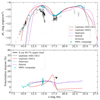 |
Fig. 1. Total intensity (top panel) and polarization (bottom panel) SED modeling for OBS3. The simultaneous observations from the MWL campaign are shown in cyan. The archival observations from the Space Science Data Center are shown in black. For both flux and polarization degree, we show the median and standard deviation in different frequencies within the IXPE observation. The lines corresponding to the different emission models are listed in the legend. |
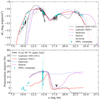 |
Fig. 5. Total intensity (top panel) and polarization (bottom panel) SED modeling for OBS4. Symbols and colors are the same as in Fig. 1. |
4. Discussion and conclusions
We used simultaneous observations from IXPE’s MWL campaigns (Peirson et al. 2023; Agudo et al. 2025) to study the total intensity and polarization SED of BL Lac in different synchrotron peak and γ-ray flux states. We used the optical polarization as a benchmark for the ordering of magnetic fields and aimed to simultaneously model the MWL spectrum and polarization degree. We find that both the leptonic models and the hybrid hadronic model considered here can satisfy the MWL and polarization observations, except the X-ray constraints. For the models to satisfy the X-ray polarization upper limits, the X-ray emission in BL Lac, and consequently blazars in general, they must be dominated by inverse-Compton scattering from the relativistic electrons. Our results thus provide stringent constraints on the origin of the high-energy emission in jets.
All the one-zone model curves (SSC+EC, hybrid, and hadronic) are below the radio to far-infrared data points. This is because the radio to far-infrared emission can come from a much larger portion of the blazar jet rather than merely the blazar zone. On the other hand, the multi-zone pure SSC model can consider both the blazar zone and the large-scale jet. Hence, it fits those data points reasonably well. However, the pure SSC model generally misses the γ-ray data, suggesting the need for an EC component.
We note that the hybrid model yields a very hard spectrum in the TeV bands, due to the strong contribution from hadronic cascades. Current Cherenkov telescopes can test this scenario. If this component is not detected, then the hybrid model will be strongly disfavored. This also highlights the potential synergies between IXPE and future Cherenkov telescopes (e.g., CTAO; Boisson et al. 2021).
All the models can satisfy the X-ray polarization upper limits for OBS3, SEG1, SEG2, and SEG3. Nonetheless, the hybrid and hadronic models are disfavored. Based on our modeling for SEG1, the hadronic and hybrid models predict a roughly constant polarization degree across the IXPE band. In that case, one would expect the X-ray polarization analysis for the 2–4 keV and 2–8 keV bands to yield the same results. Instead, we observe a detection in the 2–4 keV band and a non-detection in the 2–8 keV band. This would imply that the upper half of the IXPE band (4–8 keV) is dominated by a different process than the lower half. Additionally, the 2–4 keV polarization is not detected in SEG2 and SEG3, showing that the polarization is variable within a few days in the observer’s frame, corresponding to roughly one month in the comoving frame of the blazar zone. The proton energy that produces the X-ray emission via either proton synchrotron or hadronic cascades is a few PeV. Both the flux and polarization variability are controlled by magnetic field and particle evolution. If the magnetic field changes fast enough, the flux variability for electron synchrotron and proton synchrotron can be comparable. However, due to the faster cooling of electrons, changes in the magnetic field will significantly enhance and/or reduce local electron synchrotron cooling and, thus, the electron particle energy distribution, which is reflected in a comparably fast change in the polarization. On the other hand, protons cool much more slowly; therefore, changes in the magnetic field hardly alter the proton distribution. Consequently, the hadronic polarization variability should always be slower than the electron synchrotron polarization variations (Zhang et al. 2016, 2019, 2024). Based on the hybrid and hadronic model parameters (see Tables C.3 and C.4), the cooling timescale for protons is ≳30 yr in the comoving frame. If the X-ray and γ-ray emission are of hadronic origin, then the hadronic polarization is unlikely to change within OBS3 as shown in Zhang et al. (2016). Therefore, hybrid and hadronic models cannot adequately and consistently explain OBS3, SEG1, SEG2, and SEG3. We note that none of the models can fully explain the high 2–4 keV polarization. We suggest that it may result from a highly inhomogeneous synchrotron contribution from a localized region with very ordered magnetic fields (e.g., a shock), which is not fully captured by the multi-zone pure SSC model or the semi-analytical multi-zone polarization post-processing of the SSC+EC model. The derived parameters for both leptonic models roughly yield an equipartition between the electron energy and magnetic energy densities (see Tables C.1 and C.2). Since the energy in protons is unconstrained in the leptonic models, it is unclear how magnetized the blazar zone is or what drives the particle acceleration. But given the high 2–4 keV polarization in SEG1, the emission region is likely energy stratified.
Our strongest constraints come from OBS4, which combines the lowest X-ray upper limit and the highest optical polarization degree. We find that a pure hadronic model produces an X-ray polarization degree that is too high compared to the observations and, therefore, can be ruled out. Instead, the X-ray polarization upper limit can be satisfied with models invoking SSC+EC or SSC+hadronic emission, where SSC dominates the IXPE band. Whether the radiative output at higher energies is dominated by leptonic or hadronic processes is still a mystery. Interestingly, in our modeling, leptonic processes continue to have a low polarization degree at higher (> MeV) energies, whereas hadronic processes are typically a factor of two higher. Simultaneous X-ray (IXPE) and γ-ray polarization observations with future missions (e.g., COSI, Tomsick et al. 2024; AMEGO, Rani et al. 2019) could allow us to differentiate between emission scenarios.
Acknowledgments
We thank the anonymous referee for helpful comments that helped improve the paper. The Imaging X-ray Polarimetry Explorer (IXPE) is a joint US and Italian mission. The US contribution is supported by the National Aeronautics and Space Administration (NASA) and led and managed by its Marshall Space Flight Center (MSFC), with industry partner Ball Aerospace (contract NNM15AA18C) – now, BAE Systems. The Italian contribution is supported by the Italian Space Agency (Agenzia Spaziale Italiana, ASI) through contract ASI-OHBI-2022-13-I.0, agreements ASI-INAF-2022-19-HH.0 and ASI-INFN-2017.13-H0, and its Space Science Data Center (SSDC) with agreements ASI-INAF-2022-14-HH.0 and ASI-INFN 2021-43-HH.0, and by the Istituto Nazionale di Astrofisica (INAF) and the Istituto Nazionale di Fisica Nucleare (INFN) in Italy. This research used data products provided by the IXPE Team (MSFC, SSDC, INAF, and INFN) and distributed with additional software tools by the High-Energy Astrophysics Science Archive Research Center (HEASARC), at NASA Goddard Space Flight Center (GSFC). Based on observations obtained with XMM-Newton, an ESA science mission with instruments and contributions directly funded by ESA Member States and NASA. We acknowledge the use of public data from the Swift data archive. Some of the data are based on observations collected at the Observatorio de Sierra Nevada; which is owned and operated by the Instituto de Astrofísica de Andalucía (IAA-CSIC); and at the Centro Astronómico Hispano en Andalucía (CAHA); which is operated jointly by Junta de Andalucía and Consejo Superior de Investigaciones Científicas (IAA-CSIC). The Perkins Telescope Observatory, located in Flagstaff, AZ, USA, is owned and operated by Boston University. This research was partially supported by the Bulgarian National Science Fund of the Ministry of Education and Science under grants KP-06-H68/4 (2022) and KP-06-H88/4 (2024). The Liverpool Telescope is operated on the island of La Palma by Liverpool John Moores University in the Spanish Observatorio del Roque de los Muchachos of the Instituto de Astrofisica de Canarias with financial support from the UKRI Science and Technology Facilities Council (STFC) (ST/T00147X/1). This research has made use of data from the RoboPol program, a collaboration between Caltech, the University of Crete, IA-FORTH, IUCAA, the MPIfR, and the Nicolaus Copernicus University, which was conducted at Skinakas Observatory in Crete, Greece. The data in this study include observations made with the Nordic Optical Telescope, owned in collaboration by the University of Turku and Aarhus University, and operated jointly by Aarhus University, the University of Turku and the University of Oslo, representing Denmark, Finland and Norway, the University of Iceland and Stockholm University at the Observatorio del Roque de los Muchachos, La Palma, Spain, of the Instituto de Astrofisica de Canarias. The data presented here were obtained in part with ALFOSC, which is provided by the Instituto de Astrofísica de Andalucía (IAA) under a joint agreement with the University of Copenhagen and NOT. The Submillimeter Array (SMA) is a joint project between the Smithsonian Astrophysical Observatory and the Academia Sinica Institute of Astronomy and Astrophysics and is funded by the Smithsonian Institution and the Academia Sinica. Maunakea, the location of the SMA, is a culturally important site for the indigenous Hawaiian people; we are privileged to study the cosmos from its summit. The POLAMI observations reported here were carried out at the IRAM 30m Telescope. IRAM is supported by INSU/CNRS (France), MPG (Germany) and IGN (Spain). The KVN is a facility operated by the Korea Astronomy and Space Science Institute. The KVN operations are supported by KREONET (Korea Research Environment Open NETwork) which is managed and operated by KISTI (Korea Institute of Science and Technology Information). Partly based on observations with the 100-m telescope of the MPIfR (Max-Planck-Institut für Radioastronomie) at Effelsberg. Observations with the 100-m radio telescope at Effelsberg have received funding from the European Union’s Horizon 2020 research and innovation programme under grant agreement No 101004719 (ORP). The IAA-CSIC co-authors acknowledge financial support from the Spanish “Ministerio de Ciencia e Innovación” (MCIN/AEI/ 10.13039/501100011033) through the Center of Excellence Severo Ochoa award for the Instituto de Astrofíisica de Andalucía-CSIC (CEX2021-001131-S), and through grants PID2019-107847RB-C44 and PID2022-139117NB-C44. I.L was supported by the NASA Postdoctoral Program at the Marshall Space Flight Center, administered by Oak Ridge Associated Universities under contract with NASA. B. A.-G., I.L were funded by the European Union ERC-2022-STG – BOOTES – 101076343. Views and opinions expressed are however those of the author(s) only and do not necessarily reflect those of the European Union or the European Research Council Executive Agency. Neither the European Union nor the granting authority can be held responsible for them. HZ is supported by NASA under award number 80GSFC21M0002. HZ’s work is supported by Fermi GI program cycle 16 under the award number 22-FERMI22-0015. This work has been partially supported by the ASI-INAF program I/004/11/4. The research at Boston University was supported in part by National Science Foundation grant AST-2108622, NASA Fermi Guest Investigator grant 80NSSC23K1507, NASA NuSTAR Guest Investigator grant 80NSSC24K0547, and NASA Swift Guest Investigator grant 80NSSC23K1145. This work was supported by NSF grant AST-2109127. E. L. was supported by Academy of Finland projects 317636 and 320045. We acknowledge funding to support our NOT observations from the Finnish Centre for Astronomy with ESO (FINCA), University of Turku, Finland (Academy of Finland grant nr 306531). S. Kang, S.-S. Lee, W. Y. Cheong, S.-H. Kim, and H.-W. Jeong were supported by the National Research Foundation of Korea (NRF) grant funded by the Korea government (MIST) (2020R1A2C2009003, RS-2025-00562700). CC acknowledges support by the European Research Council (ERC) under the HORIZON ERC Grants 2021 programme under grant agreement No. 101040021. This work was supported by JST, the establishment of university fellowships towards the creation of science technology innovation, Grant Number JPMJFS2129. D.B. acknowledge support from the European Research Council (ERC) under the European Unions Horizon 2020 research and innovation program under grant agreement No. 771282. J.O.-S. acknowledges founding from the Istituto Nazionale di Fisica Nucleare (INFN) Cap. U.1.01.01.01.009.
References
- Abdollahi, S., Acero, F., Ackermann, M., et al. 2020, ApJS, 247, 33 [Google Scholar]
- Agudo, I., Thum, C., Molina, S. N., et al. 2018, MNRAS, 474, 1427 [NASA ADS] [CrossRef] [Google Scholar]
- Agudo, I., Liodakis, I., Otero-Santos, J., et al. 2025, ApJ, 985, L15 [Google Scholar]
- Ajello, M., Angioni, R., Axelsson, M., et al. 2020, ApJ, 892, 105 [NASA ADS] [CrossRef] [Google Scholar]
- Bachev, R., Tripathi, T., Gupta, A. C., et al. 2023, MNRAS, 522, 3018 [NASA ADS] [CrossRef] [Google Scholar]
- Blandford, R., Meier, D., & Readhead, A. 2019, ARA&A, 57, 467 [NASA ADS] [CrossRef] [Google Scholar]
- Blinov, D., Kiehlmann, S., Pavlidou, V., et al. 2021, MNRAS, 501, 3715 [NASA ADS] [CrossRef] [Google Scholar]
- Boisson, C., Brown, A. M., Burtovoi, A., et al. 2021, arXiv e-prints [arXiv:2106.05971] [Google Scholar]
- Böttcher, M., Reimer, A., Sweeney, K., & Prakash, A. 2013, ApJ, 768, 54 [Google Scholar]
- de Jaeger, T., Shappee, B. J., Kochanek, C. S., et al. 2023, MNRAS, 519, 6349 [NASA ADS] [CrossRef] [Google Scholar]
- Hovatta, T., & Lindfors, E. 2019, New Astron. Rev., 87, 101541 [CrossRef] [Google Scholar]
- IceCube Collaboration (Aartsen, M.G., et al.) 2018, Science, 361, eaat1378 [NASA ADS] [CrossRef] [Google Scholar]
- Kang, S., Lee, S.-S., & Byun, D.-Y. 2015, J. Korean Astron. Soc., 48, 257 [NASA ADS] [CrossRef] [Google Scholar]
- Kouch, P. M., Liodakis, I., Middei, R., et al. 2024, A&A, 689, A119 [NASA ADS] [CrossRef] [EDP Sciences] [Google Scholar]
- Kouch, P. M., Liodakis, I., Fenu, F., et al. 2025, A&A, 695, A99 [NASA ADS] [CrossRef] [EDP Sciences] [Google Scholar]
- Kraus, A., Krichbaum, T. P., Wegner, R., et al. 2003, A&A, 401, 161 [NASA ADS] [CrossRef] [EDP Sciences] [Google Scholar]
- Liodakis, I., Hovatta, T., Huppenkothen, D., et al. 2018, ApJ, 866, 137 [Google Scholar]
- Liodakis, I., Peirson, A. L., & Romani, R. W. 2019a, ApJ, 880, 29 [NASA ADS] [CrossRef] [Google Scholar]
- Liodakis, I., Romani, R. W., Filippenko, A. V., Kocevski, D., & Zheng, W. 2019b, ApJ, 880, 32 [NASA ADS] [CrossRef] [Google Scholar]
- Liodakis, I., Marscher, A. P., Agudo, I., et al. 2022, Nature, 611, 677 [CrossRef] [Google Scholar]
- Mannheim, K. 1993, Phys. Rev. D, 48, 2408 [NASA ADS] [CrossRef] [Google Scholar]
- Marshall, H. L., Liodakis, I., Marscher, A. P., et al. 2024, ApJ, 972, 74 [NASA ADS] [CrossRef] [Google Scholar]
- Middei, R., Liodakis, I., Perri, M., et al. 2023, ApJ, 942, L10 [NASA ADS] [CrossRef] [Google Scholar]
- Mondal, A., Sar, A., Kundu, M., Chatterjee, R., & Majumdar, P. 2025, ApJ, 978, 43 [Google Scholar]
- Myserlis, I., Angelakis, E., Kraus, A., et al. 2018, A&A, 609, A68 [NASA ADS] [CrossRef] [EDP Sciences] [Google Scholar]
- Nilsson, K., Lindfors, E., Takalo, L. O., et al. 2018, A&A, 620, A185 [NASA ADS] [CrossRef] [EDP Sciences] [Google Scholar]
- Otero-Santos, J., Piirola, V., Escudero Pedrosa, J., et al. 2024, AJ, 167, 137 [Google Scholar]
- Panopoulou, G., Tassis, K., Blinov, D., et al. 2015, MNRAS, 452, 715 [Google Scholar]
- Peirson, A. L., & Romani, R. W. 2019, ApJ, 885, 76 [NASA ADS] [CrossRef] [Google Scholar]
- Peirson, A. L., Liodakis, I., & Romani, R. W. 2022, ApJ, 931, 59 [CrossRef] [Google Scholar]
- Peirson, A. L., Negro, M., Liodakis, I., et al. 2023, ApJ, 948, L25 [NASA ADS] [CrossRef] [Google Scholar]
- Poutanen, J. 1994, ApJS, 92, 607 [NASA ADS] [CrossRef] [Google Scholar]
- Ramaprakash, A. N., Rajarshi, C. V., Das, H. K., et al. 2019, MNRAS, 485, 2355 [NASA ADS] [CrossRef] [Google Scholar]
- Rani, B., Zhang, H., Hunter, S. D., et al. 2019, BAAS, 51, 348 [Google Scholar]
- Shrestha, M., Steele, I. A., Piascik, A. S., et al. 2020, MNRAS, 494, 4676 [NASA ADS] [CrossRef] [Google Scholar]
- Tomsick, J. A., Boggs, S. E., Zoglauer, A., et al. 2024, 38th International Cosmic Ray Conference, Nagoya, Japan, 745 [Google Scholar]
- Weisskopf, M. C., Soffitta, P., Baldini, L., et al. 2022, JATIS, 8, 026002 [NASA ADS] [Google Scholar]
- Zhang, H., & Böttcher, M. 2013, ApJ, 774, 18 [NASA ADS] [CrossRef] [Google Scholar]
- Zhang, H., Diltz, C., & Böttcher, M. 2016, ApJ, 829, 69 [NASA ADS] [Google Scholar]
- Zhang, H., Fang, K., Li, H., et al. 2019, ApJ, 876, 109 [NASA ADS] [CrossRef] [Google Scholar]
- Zhang, H., Böttcher, M., & Liodakis, I. 2024, ApJ, 967, 93 [NASA ADS] [Google Scholar]
Appendix A: Spectral energy distribution models
 |
Fig. A.1. Spectral energy distribution modeling for OBS3: The one-zone leptonic model (top left), the multi-zone leptonic model (top right), the hadronic model (bottom left), and the hybrid model (bottom right). The simultaneous observations from the MWL campaign are shown in cyan. The archival observations from the Space Science Data Center are shown in black. The lines corresponding to the different emission components are listed in the legend. |
Appendix B: Spectral polarization models
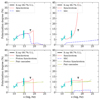 |
Fig. B.1. Spectral polarization modeling for OBS3: The one-zone leptonic model (top left), the multi-zone leptonic model (top right), the hadronic model (bottom left), and the hybrid model (bottom right). The simultaneous observations from the MWL campaign are shown in cyan. The archival observations from the Space Science Data Center are shown in black. The lines corresponding to the different emission components are listed in the legend. |
Appendix C: Spectral energy distribution model parameters
Parameter values for different observations for the pure SSC multi-zone model at the base of the jet.
SSC+EC model parameters across all observations.
SSC+hadronic model parameters across all observations.
Hadronic model parameters across all observations.
All Tables
Parameter values for different observations for the pure SSC multi-zone model at the base of the jet.
All Figures
|
Fig. 1. Total intensity (top panel) and polarization (bottom panel) SED modeling for OBS3. The simultaneous observations from the MWL campaign are shown in cyan. The archival observations from the Space Science Data Center are shown in black. For both flux and polarization degree, we show the median and standard deviation in different frequencies within the IXPE observation. The lines corresponding to the different emission models are listed in the legend. |
| In the text | |
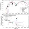 |
Fig. 2. Same as Fig. 1, but for SEG1. |
| In the text | |
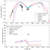 |
Fig. 3. Same as Fig. 1, but for SEG2. |
| In the text | |
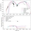 |
Fig. 4. Same as Fig. 1, but for SEG3. |
| In the text | |
|
Fig. 5. Total intensity (top panel) and polarization (bottom panel) SED modeling for OBS4. Symbols and colors are the same as in Fig. 1. |
| In the text | |
|
Fig. A.1. Spectral energy distribution modeling for OBS3: The one-zone leptonic model (top left), the multi-zone leptonic model (top right), the hadronic model (bottom left), and the hybrid model (bottom right). The simultaneous observations from the MWL campaign are shown in cyan. The archival observations from the Space Science Data Center are shown in black. The lines corresponding to the different emission components are listed in the legend. |
| In the text | |
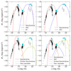 |
Fig. A.2. Same as Fig. A.1, but for SEG1. |
| In the text | |
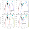 |
Fig. A.3. Same as Fig. A.1, but for SEG2. |
| In the text | |
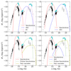 |
Fig. A.4. Same as Fig. A.1, but for SEG3. |
| In the text | |
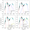 |
Fig. A.5. Same as Fig. A.1 but for OBS4. |
| In the text | |
|
Fig. B.1. Spectral polarization modeling for OBS3: The one-zone leptonic model (top left), the multi-zone leptonic model (top right), the hadronic model (bottom left), and the hybrid model (bottom right). The simultaneous observations from the MWL campaign are shown in cyan. The archival observations from the Space Science Data Center are shown in black. The lines corresponding to the different emission components are listed in the legend. |
| In the text | |
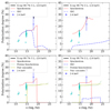 |
Fig. B.2. Same as Fig. B.1, but for SEG1. |
| In the text | |
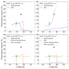 |
Fig. B.3. Same as Fig. B.1, but for SEG2. |
| In the text | |
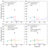 |
Fig. B.4. Same as Fig. B.1, but for SEG3. |
| In the text | |
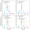 |
Fig. B.5. Same as Fig. B.1, but for OBS4. |
| In the text | |
Current usage metrics show cumulative count of Article Views (full-text article views including HTML views, PDF and ePub downloads, according to the available data) and Abstracts Views on Vision4Press platform.
Data correspond to usage on the plateform after 2015. The current usage metrics is available 48-96 hours after online publication and is updated daily on week days.
Initial download of the metrics may take a while.