| Issue |
A&A
Volume 658, February 2022
|
|
|---|---|---|
| Article Number | A179 | |
| Number of page(s) | 27 | |
| Section | Astrophysical processes | |
| DOI | https://doi.org/10.1051/0004-6361/202141453 | |
| Published online | 21 February 2022 | |
Type Iax supernovae from deflagrations in Chandrasekhar mass white dwarfs
1
Heidelberger Institut für Theoretische Studien, Schloss-Wolfsbrunnenweg 35, 69118 Heidelberg, Germany
e-mail: This email address is being protected from spambots. You need JavaScript enabled to view it.
2
Zentrum für Astronomie der Universität Heidelberg, Institut für Theoretische Astrophysik, Philosophenweg 12, 69120 Heidelberg, Germany
3
School of Mathematics and Physics, Queen’s University Belfast, Belfast BT7 1NN, UK
4
Institute of Theoretical Physics and Astrophysics, University of Würzburg, 97074 Würzburg, Germany
5
Max Planck Computing and Data Facility, Gießenbachstr. 2, 85748 Garching, Germany
Received:
2
June
2021
Accepted:
22
November
2021
Abstract
Context. Due to the ever increasing number of observations during the past decades, Type Ia supernovae are nowadays regarded as a heterogeneous class of optical transients consisting of several subtypes. One of the largest of these subclasses is the class of Type Iax supernovae. They have been suggested to originate from pure deflagrations in carbon-oxygen Chandrasekhar mass white dwarfs because the outcome of this explosion scenario is in general agreement with their subluminous nature.
Aims. Although a few deflagration studies have already been carried out, the full diversity of the class has not been captured yet. This, in particular, holds for the faint end of the subclass. We therefore present a parameter study of single-spot ignited deflagrations in Chandrasekhar mass white dwarfs varying the location of the ignition spark, the central density, the metallicity, and the composition of the white dwarf. We also explore a rigidly rotating progenitor to investigate whether the effect of rotation can spawn additional trends.
Methods. We carried out three-dimensional hydrodynamic simulations employing the LEAFS code. Subsequently, detailed nucleosynthesis results were obtained with the nuclear network code YANN. In order to compare our results to observations, we calculated synthetic spectra and light curves with the ARTIS code.
Results. The new set of models extends the range in brightness covered by previous studies to the lower end. Our single-spot ignited explosions produce 56Ni masses from 5.8 × 10⁻³ to 9.2 × 10⁻² M⊙. In spite of the wide exploration of the parameter space, the main characteristics of the models are primarily driven by the mass of 56Ni and form a one-dimensional sequence. Secondary parameters seem to have too little impact to explain the observed trend in the faint part of the Type Iax supernova class. We report kick velocities of the gravitationally bound explosion remnants from 6.9 to 369.8 km s−1. The magnitude as well as the direction of the natal kick is found to depend on the strength of the deflagration.
Conclusions. This work corroborates the results of previous studies of deflagrations in Chandrasekhar mass white dwarfs. The wide exploration of the parameter space in initial conditions and viewing angle effects in the radiative transfer lead to a significant spread in the synthetic observables. The trends in observational properties toward the faint end of the class are, however, not reproduced. This motivates a quantification of the systematic uncertainties in the modeling procedure and the influence of the 56Ni-rich bound remnant to get to the bottom of these discrepancies. Moreover, while the pure deflagration scenario remains a favorable explanation for bright and intermediate luminosity Type Iax supernovae, our results suggest that other mechanisms also contribute to this class of events.
Key words: hydrodynamics / radiative transfer / instabilities / white dwarfs / supernovae: general / methods: numerical
© ESO 2021
1. Introduction
Type Ia supernovae (SNe Ia) have, for a long time, been thought to form a rather homogeneous class of cosmic explosions. In fact, the majority of events show similar photometric and spectroscopic behavior. Their light curves follow an empirical width-luminosity relation (WLR, Phillips relation, Phillips 1993), associating broad shapes with bright events. This property makes these so-called Branch-normal supernovae (Branch et al. 1993, 2006) standardizable candles, widely employed for distance measurements (Riess et al. 1996; Schmidt et al. 1998; Perlmutter et al. 1999; Jha et al. 2007). However, the increasing number of observations over the past decades led to the detection of outliers and eventually called for the introduction of several subclasses of SNe Ia. These subtypes are believed to share the thermonuclear origin with normal SNe Ia, that is, the disruption of a carbon-oxygen (CO, in some cases also oxygen-neon (ONe), Marquardt et al. 2015; Kashyap et al. 2018) white dwarf (WD) due to explosive nuclear burning, but they exhibit clear differences in some characterizing properties (see Taubenberger 2017 for a review).
The largest of these subclasses of SNe Ia is the subluminous supernovae of Type Iax (SNe Iax), with more than ∼50 members observed. According to Foley et al. (2013), SNe Iax might account for about 31% of all SNe Ia while Li et al. (2011) and White et al. (2015) estimated their rate to be ∼5% (Jha 2017). The typical object for this class is SN 2002cx (Li et al. 2003), and, therefore, at least the brighter objects are also called 02cx-like events. Foley et al. (2013) named these transients SNe Iax and defined the key observational features of this class as follows: (i) no evidence of hydrogen in any spectrum, (ii) lower maximum-brightness photospheric velocity than any normal SN Ia, (iii) low absolute magnitude near maximum light in relation to the width of its light curve (i.e., they fall below the WLR), and (iv) spectra similar to SN 2002cx at comparable epochs.
While the first criterion represents the usual distinction between SNe Ia and supernovae of Type II, the second and third requirements suggest the production of only a small amount of energy. The optical emission from SNe Ia is powered by the radioactive decay of 56Ni to 56Co in the early phase, and, therefore, their brightness is directly linked to the ejected mass of 56Ni. Peak absolute brightnesses derived from observations range between −14 ≥ MV ≥ −19, inferred 56Ni masses lie between 0.003 and 0.27 M⊙ (Foley et al. 2013; Jha 2017), and ejected masses Mej between 0.15 M⊙ for the faintest members of this class, such as SN 2008ha (Foley et al. 2009), and up to approximately MCh for the brightest events (e.g., SN 2012Z, Stritzinger et al. 2015). Normal SNe Ia, in contrast, eject between 0.3 and 0.9 M⊙ of 56Ni (Hillebrandt et al. 2013). In addition, ejecta velocities are significantly lower than those of normal SNe Ia and usually fall below 8000 km s−1 down to ≲2000 km s−1 for the faintest SNe Iax (Foley et al. 2009). However, B-band light curve decline rates span a similar range compared to normal events, but they cannot be connected to the corresponding brightness via the WLR, and, thus, SNe Iax are not employed as distance indicators. The shape of their light curves in the optical regime resembles normal SNe Ia while the prominent second peak in the near-infrared (NIR) bands (IJHK; Hamuy et al. 1996; Kasen 2006) is absent in SNe Iax (Foley & Kirshner 2013; Magee et al. 2016; Jha 2017). Also the redder bands tend to decline slower compared to lower wavelengths (Tomasella et al. 2016) and show a larger variation in decline rates compared to normal SNe Ia. There is also a loose corellation between photosperic velocities and peak magnitudes (McClelland et al. 2010; Foley & Kirshner 2013), that is, brighter events also show higher expansion velocities, challenged only by some outliers such as SN 2009ku (Narayan et al. 2011) and SN 2014ck (Tomasella et al. 2016). In addition, Magee et al. (2016) study the rise times of SNe Iax (trise = 9 − 28 d) and find an increasing trend with peak r-band magnitude, but again with a clear outlier, namely SN 2009eoi.
The near maximum spectrum of SN 2002cx, and, by definition those of other SNe Iax, is characterized by prominent Fe III lines and relatively weak signs of IMEs, for example, Si II and S II (Branch et al. 2004). Surprisingly, this is quite similar to the overluminous and rapidly expanding SN 1991T-like events. The photospheric velocity, however, is very low (∼7000 km s−1) making it easier to identify individual species since absorption and emission features are broadened less. About two weeks after maximum the Si II feature has disappeared and the spectrum is dominated by singly ionized iron group elements (IGEs). Until 56 d the spectrum resembles those of normal SNe Ia at slightly later times and has not turned nebular yet (Branch et al. 2004). The late-time spectra of SN 2002cx (227 and 277 d) were examined by Jha et al. (2006). They found that the spectra did not change significantly after 56 d post maximum and deviate significantly from those of normal SNe Ia. Instead of being dominated by forbidden lines of Fe and Co typical for nebular spectra they exhibit P Cygni features of Fe II but also IMEs and potentially signs of oxygen. Foley et al. (2016) also state that late-time spectra of SNe Iax only show minor changes over time and that differences among the subclass originate primarily from different expansion velocities. Finally, they find clear signs of Ni II pointing toward a significant amount of stable Ni in the ejecta.
Several different progenitor systems and explosion mechanisms have been proposed for thermonuclear supernovae during the past decades. The explosion of the WD is triggered by the interaction with a hydrogen or helium-rich companion (single-degenerate scenario, Whelan & Iben 1973) or another WD (double-degenerate scenario, Iben & Tutukov 1984). Furthermore, the explosion is caused by a thermonuclear runaway in degenerate matter resulting in either a subsonic deflagration or a supersonic detonation. The propagation of a deflagration is mediated by heat conduction while a detonation proceeds as a shock wave. Moreover, a spontaneous transition from a deflagration to a detonation has been proposed by Blinnikov & Khokhlov (1986), Khokhlov (1989) and was studied by Khokhlov (1991), Gamezo et al. (2005), Röpke (2007), and Seitenzahl et al. (2013), for instance. Comprehensive summaries of the whole “zoo” of possible SN Ia explosion scenarios can be found in reviews, for example, Wang & Han (2012), Hillebrandt et al. (2013), Livio & Mazzali (2018), Röpke & Sim (2018), and Soker (2019).
One promising scenario for explaining SNe Iax is a MCh pure deflagration as proposed by Branch et al. (2004, 2006) for SN 2002cx and Chornock et al. (2006) and Phillips et al. (2007) for SN 2005hk. Recently, deflagrations in hybrid carbon-oxygen-neon (CONe) instead of pure CO WDs have also been considered as progenitors for SNe Iax (Denissenkov et al. 2015; Kromer et al. 2015; Bravo et al. 2016). This scenario naturally accounts for many characteristics of SNe Iax. Most notably, the simulations of these explosions do not eject enough 56Ni to reach the absolute magnitudes of normal SNe Ia, and, depending on the ignition configuration, do not disrupt the whole WD, but leave behind a bound remnant (Jordan et al. 2012; Kromer et al. 2013; Fink et al. 2014). Foley et al. (2014) speculate about the existence of such a bound remnant in SN 2008ha and suggest that it emits a wind preventing the spectra from transitioning to the nebular phase which is one of the most characterisitc properties of SN Iax spectra. Moreover, evidence for a bound remnant was also found in the slowly declining late-time light curve of SN 2014dt by Kawabata et al. (2018) and very recently in SN 2019muj (Kawabata et al. 2021). The latter also employ their analytical, phenomenological light curve model to other SNe Iax and conclude that their late-time light curves are well matched assuming radiating burning products at low velocities. The radiation of gravitationally bound or slowly expanding 56Ni is also suspected to contribute to the light curves and spectra by Foley et al. (2016), Magee et al. (2016), and Shen & Schwab (2017).
These deflagrations lead to photospheric velocities in the observed range below those of normal SNe Ia. The detection of IGEs and IMEs in their spectra at all times and the lack of a second maximum in the NIR ligth curves (see Kasen 2006) suggests a rather mixed ejecta structure which is a natural outcome of a turbulent deflagration. However, the assumption of completely mixed ejecta in some bright SNe Iax has been challenged by Stritzinger et al. (2015), Barna et al. (2017, 2018). Therefore, a pulsational delayed detonation (Höflich & Khokhlov 1996) scenario was proposed for the most energetic SNe Iax (Stritzinger et al. 2015). However, the need for stratification in the moderately bright SN 2019muj was not found to be very strong for all elements except carbon in the outer layers (Barna et al. 2021). It should be noted that their approach is only sensitive to velocities between 3600 and ∼6500 km s−1. In this region, their stratified template model does not differ significantly from well mixed deflagration ejecta.
The single degenerate scenario suffers the problem of stripped hydrogen or helium from the companion star: It is expected that the explosion of the WD will remove material from its donor which should be seen in the late-time spectra (Pakmor et al. 2008; Lundqvist et al. 2013; Bauer et al. 2019). Since SNe Iax are less energetic than normal SNe Ia, Liu et al. (2013) and Zeng et al. (2020) argue that the stripped hydrogen or helium might stay below the detection limit. Magee et al. (2019) also look for helium features in SNe Iax and find that their NIR spectra are compatible with only very small amounts of helium and that it is easier to detect in fainter models. Another hint toward the MCh scenario for SNe Iax is the possible detection of a bright helium-star at the location of SN 2012Z (McCully et al. 2014a) because accretion of helium is a plausible way for a WD to reach MCh. McCully et al. (2022) present very late time observations of SN 2012Z up to 1425 d after maximum light. They find that the event is still about a factor of two brighter than pre-explosion and attribute this either to the shock-heated companion, a bound remnant (see above), or radioactive decay of long-lived isotopes other than 56, 57Co. In addition, the recently detected hypervelocity WDs with an unusual composition (Raddi et al. 2019) have also been associated with the bound remnant WD cores found in simulations of MCh deflagrations. These characteristics make MCh deflagrations a promising scenario for SNe Iax and motivate a deeper investigation of this model. Moreover, their occurrence in star-forming regions of late type galaxies are in line with a WD accreting helium from its donor star (Lyman et al. 2018).
SNe Ia contribute substantially to cosmic nucleosynthesis (Nomoto et al. 2013; Thielemann et al. 2018) and it is widely accepted that they are required for the production of the neutron-rich element manganese alongside core-collapse supernovae (Seitenzahl et al. 2013; Kobayashi et al. 2006, 2020; Lach et al. 2020). Explosions of MCh WDs are able to produce supersolar amounts of Mn relative to Fe in their innermost, that is, densest, parts in normal freeze-out from nuclear statistical equilibrium (NSE, see Woosley et al. 1973; Hix & Thielemann 1999; Seitenzahl et al. 2009; Bravo 2019) since the rate of electron captures increases with density (Chamulak et al. 2008; Piro & Bildsten 2008; Brachwitz et al. 2000). Therefore, if SNe Iax originate from deflagrations in MCh WDs they are promising candidates for the enrichment of the Universe with Mn. Recently, double-detonation models for SNe Ia came into the focus as a production site of Mn, but they can probably not completely replace explosions of MCh WDs (Lach et al. 2020; Gronow et al. 2021).
Simulations of deflagrations in MCh CO WDs with a clear relation to SNe Iax have been carried out by Jordan et al. (2012), Long et al. (2014), Kromer et al. (2013, 2015), Fink et al. (2014), and Leung & Nomoto (2020). We summarize the findings and shortcomings of this previous work in more detail in Sect. 2.
As an alternative scenario, SN 2008ha has also been speculated to be a core-collapse SN (Valenti et al. 2009) or even a failed detonation of an ONe WD merging with a CO secondary (Kashyap et al. 2018). Fernández & Metzger (2013) also bring a detonation ignited in a WD-neutron star merger event into play for SNe Iax. While the historic SN Iax remnant SN 1181 is believed to originate from an ONe-CO WD merger (Oskinova et al. 2020; Ritter et al. 2021) the SN remnant Sgr A East has recently been associated with a failed deflagration producing a SN Iax (Zhou et al. 2021). Hence, the question whether it is possible to explain the entire class of SNe Iax in the framework of the pure deflagration in a MCh WD model remains.
To address this question, we present an extensive set of three-dimensional (3D) full-star simulations of deflagrations in MCh CO WDs. Since the most realistic ignition configuration consists of only one spot (Kuhlen et al. 2006; Zingale et al. 2009; Nonaka et al. 2012) we restrict our suite of simulations to single-spot ignition. The location of this ignition spark and the central density are systematically varied to investigate the dependence on these parameters. With this study, we aim to extend the set of deflagration models toward the faintest events of the SNe Iax class and systematically determine expected properties of bound remnants. Furthermore, we aim to explore whether the restriction to a single ignition spark but variation of other parameters can change the general characteristics of pure deflagration models.
The paper is structured as follows: We give a summary of previous deflagration studies in Sect. 2 followed by a short overview of the numerical methods used to simulate the explosion in Sect. 3. Subsequently, we describe our initial models in Sect. 4 and discuss the results of the hydrodynamic simulations in Sect. 5. The outcome of the radiative transfer (RT) calculations is compared to observations in Sect. 6. Finally, we wrap up our findings and conclusions in Sect. 7.
2. Previous work
In the following we summarize the results of various works concerning the modeling of deflagrations in MCh WDs in connection to SNe Iax. These results help to understand the open questions and shortcomings of the currently available simulations and also guide the choice of parameters for the study carried out in our work.
2.1. Jordan et al. (2012)
Jordan et al. (2012, hereafter J12) present a set of models of pure deflagrations in CO MCh WDs. Since their models fail to ignite a delayed detonation and do not unbind the WD, they call these explosions failed-detonation SNe. They carry out two-dimensional (2D) as well as 3D hydrodynamic simulations, but do neither present detailed nucleosynthesis yields nor radiative transport calculations. Their MCh WD (1.365 M⊙, ρc = 2.2 × 10⁹ g cm−3) is ignited in 63 spots of 16 km radius contained inside a sphere of 128 km radius. This sphere is located slightly off-center at distances of 48, 38, 28 and 18 km from the center of the WD. The 2D run, however, uses only four ignition sparks inside a circle with a radius of 64 km displaced by 70 km from the center of the WD.
As mentioned above, the explosion in the WD leaves behind a bound remnant in all of their simulations although 89 to 167% of the initial binding energy Ebind are released during the deflagration phase. This shows that the released energy is not necessarily distributed homogeneously and that multidimensional effects need to be taken into account. Their explosions eject between 0.23 and 1.09 M⊙ of material including 0.07 to 0.34 M⊙ of IGEs. Unfortunately, values for the production of 56Ni are not given. The ejecta velocities lie below 10 000 km s−1 and they find an asymmetric ejecta structure characterized by a surplus of burning products at the ignition side and CO fuel in the opposite direction. These features lead them to the conclusion that their models might be candidates for SNe Iax, at least for the bright SN 2002cx-like members of this subclass. However, a comparison of synthetic observables to observations is not part of this study.
Another interesting aspect investigated by J12 is the kick velocity vkick of the bound remnant. Since the explosion proceeds asymmetrically the bound core receives a kickback between 119 and 549 km s−1 which might be enough to unbind the remnant from the binary system. Together with its composition enriched by burning products such a puffed-up WD is a possible explanation for peculiar iron-rich WDs (see e.g., Provencal et al. 1998; Catalan et al. 2008 and for more recent works Vennes et al. 2017; Raddi et al. 2018a,b, 2019; Neunteufel 2020).
2.2. Long et al. (2014)
Long et al. (2014, hereafter L14) present a follow-up study of the work by J12. They utilize the same progenitor model, but also specify that they employ zero metallicity, a C/O ratio of 1 (i.e., 50% C and 50% O), and a constant temperature of T = 3 × 10⁷ K. The only free parameter is the ignition geometry. It consists again of bubbles of 16 km radius. These are confined to spheres of radius 128, 256 and 384 km located at the center of the WD. In addition, the total number of ignition sparks is varied between 63 and 3500. They carry out six 3D full-star simulations including a postprocessing step and one-dimensional (1D) RT calculations yielding synthetic light curves.
Although the total energy Etot (sum of gravitational energy Egrav, kinetic energy Ekin and internal energy EI) is positive in all their models we cannot judge whether the whole WD is unbound since it is not specified in the paper. They arrive at 56Ni masses M(56Ni) between 0.135 and 0.288 M⊙, nuclear energies Enuc between 6.78 and 9.60 × 1050 erg, and kinetic energies of the ejecta Ekin, ej between 2.44 and 5.01 × 1050 erg. The main finding is that the initial spatial density of the ignition sparks as well as the outer radius of the confining sphere determine the outcome of the simulation. As a first effect, a dense distribution leads to a high burning rate in the early phase of the flame propagation. Subsequently, the bubbles merge very rapidly, and, thus, the flame surface decreases leading to a reduction in the burning rate. Second, the gravitational acceleration, and, therefore, the buoyant force increases with radius. This causes a rapid increase in the energy production for large ignition radii but also an earlier quenching of the flame as the deflagration reaches the outer part of the WD. There is most probably an optimal choice for the number of ignition sparks per volume and the maximum ignition radius in terms of M(56Ni). The approximate number and spatial density of ignition kernels has already been estimated by Röpke et al. (2006a). In the study of L14 a modest number of bubbles (128) confined to a 128 km sphere yields the highest mass of 56Ni while very many sparks (3500) inside a 384 km sphere set the lower limit.
Finally, an examination of the synthetic light curves shows that models ignited with ∼100 kernels show more similarities to SNe Iax than vigorously ignited models with ∼1000 sparks. However, also in this study only the luminosities of bright SNe Iax are reached.
2.3. Fink et al. (2014)
The work of Fink et al. (2014, hereafter F14) was developed simultaneously to the study of L14. They conduct 14 3D full-star simulations of pure deflagrations in MCh CO WDs studying mainly the impact of the ignition geometry. In detail, they vary the number N of ignition kernels from 1 to 1600, and, for two models (N = 300 1600), they also set up a denser distribution of the bubbles. Their initial WD has a central density of 2.9 × 10⁹ g cm−3, a constant temperature of 5 × 10⁵ K, and mass fractions of X(12C) = 0.475, X(16O) = 0.50 and X(22Ne) = 0.025 to account for solar metallicity. Moreover, one model (N = 100) has also been calculated at central densities of 1.0 × 10⁹ g cm−3 and 5.5 × 10⁹ g cm−3.
Concerning the nuclear energy release and the production of 56Ni F14 arrive at the same conclusion as L14 stating that models ignited in many, densely located sparks lead to less powerful explosions compared to moderately ignited WDs. The highest amount of 56Ni is found in the model with 150 initial kernels. Moreover, the energy production in the high-density model does not differ significantly from their standard model while the low-density simulation leads to noticeable less released nuclear energy. However, the high-density model produces no more 56Ni than the low-density run because of the more neutron-rich nucleosynthesis at high densities favoring the production of stable IGEs instead.
In contrast to L14, F14 also explicitly report the existence of bound remnants for models ignited in less than 100 spots. These remnants are enriched with burning products and reach masses up to 1.32 M⊙. In addition, they also calculate their respective kick velocity, but arrive at values an order of magnitude below those presented by J12 ranging between 4.4 and 36 km s−1. They speculate that their use of an approximate monopole solver for the gravitational force might account for the differences.
F14 also present synthetic light curves and spectra resulting from 3D RT simulations concluding that models with less than 20 ignition sparks are compatible with SNe Iax. However, even their faintest explosion (N = 1) does not reach the faintest members of the SN Iax class, SN 2008ha and SN 2019gsc. The predicted spectra look very similar without a significant viewing angle dependency. Kromer et al. (2013, hereafter K13) present an in-depth analysis of the explosion ignited in 5 bubbles (Model N5). They compare N5 to SN 2005hk and state that peak luminosity, the colors at maximum and the decline in UBV bands coincide very well. Also the presence of IGEs at all times and the lack of a secondary maximum matches the characteristics of SNe Iax. However, the decline in red bands (RIJH) is significantly too fast and also the B-band rise time is too short to conform with SN 2005hk. One way to achieve a slower decline and keeping the peak luminosity fixed is to increase the ejected mass at constant M(56Ni). In addition, the influence of the bound remnant on the observables was not investigated yet.
2.4. Kromer et al. (2015)
In order to reach the faint end of the SN Iax subclass, Kromer et al. (2015, hereafter K15) carry out a deflagration simulation inside a MCh hybrid CONe WD. These progenitors had been proposed in the work of Denissenkov et al. (2013, 2015). The initial conditions, that is, density, temperature and ignition condition, were chosen to be similar to N5 of F14. The WD consists of a 0.2 M⊙ CO core and a 1.1 M⊙ ONe mantle. The burning is assumed to quench as soon as the flame reaches the ONe layer which leads to a very faint explosion ejecting only 0.014 M⊙ in total and 3.4 × 10⁻³ M⊙ of 56Ni. This provides a good fit to the peak luminosity of one of the faintest SN Iax, SN 2008ha. But still the decline (red bands) and rise of the light curve is too fast. Moreover, some line features around maximum cannot be reproduced. These deficiencies also hint toward too little ejected mass. K15 point out that the 56Ni enriched bound remnant might also have an influence on the light curve at late and possibly even early times depending on the structure of the remnant.
Bravo et al. (2016) also investigated the hybrid CONe WD scenario with 1D simulations and varying CO core masses. Their study includes pure detonations and delayed detonation models. They conclude that only delayed detonations resemble bright SNe Iax not reaching intermediate and low-luminosity events.
2.5. Leung & Nomoto (2020)
An extensive deflagration study with reference to SNe Iax was presented by Leung & Nomoto (2020, hereafter L20). They start with MCh CO and CONe WDs and vary the central density between 0.5 × 10⁹ g cm−3 and 9.0 × 10⁹ g cm−3. Furthermore, they use two different ignition conditions, that is, the c3-ignition by Reinecke et al. (1999a) and a single bubble. Unfortunately, they do not give details on the radius and the location of the ignition spark. Their simulations are conducted in 2D only and the emphasis in their work lies on the nucleosynthesis products and not on optical observables.
They report 56Ni masses between 0.20 and 0.36 M⊙ and total ejected masses between 0.92 and 1.36 M⊙. This indicates that these models can only account for the brightest SNe Iax, such as SN 2012Z.
2.6. Summary
In summary, all the deflagration studies above claim to produce models which can account for SNe Iax although not all of them carry out RT simulations and compare to observations. In these cases, the claim originates from the low explosion energies, low ejecta velocities and low masses of 56Ni compared to normal SNe Ia. It is also well known that pure deflagrations do not produce a secondary maximum in infrared bands. Studies including synthetic observables, L14, K13, F14, and K15, corroborate this claim. However, there are some discrepancies regarding the width of the model light curves (see above). Therefore, to explain the decline rate and rise times of SNe Iax and also the diversity among this subclass a much wider exploration of the parameter space is necessary.
Moreover, these modeled events cover a reasonable range in brightness, that is, ejected mass of 56Ni, but they do not account for the full diversity of the class of SNe Iax and show a bias toward bright events while the fainter objects, for instance, SN 2008ha (Foley et al. 2009), SN 2010ae (Stritzinger et al. 2014), and SN 2019gsc (Srivastav et al. 2020; Tomasella et al. 2020) are not reached. One of the major shortcoming of the works mentioned above is their use of the ignition configuration, that is, the location, shape, size and number of the initial ignition kernels, as a free parameter to control the strength of the deflagration. This is in strong contrast to the works of Zingale et al. (2011) and Nonaka et al. (2012) which suggest the ignition in one spark off-center.
3. Numerical methods
For the hydrodynamic simulations we employ the LEAFS code which has already been successfully used for a large number of explosion simulations (e.g., Röpke & Hillebrandt 2005; Röpke et al. 2007; Seitenzahl et al. 2013; Fink et al. 2014, 2018; Ohlmann et al. 2014; Marquardt et al. 2015). It is based on the Prometheus code by Fryxell et al. (1989) that has been extended and adapted by Reinecke et al. (1999a) to simulate SNe Ia. For solving the reactive Euler equations it takes a finite volume approach using the piecewise parabolic scheme by Colella & Woodward (1984). In order to treat flame fronts as discontinuities, the level-set technique (Osher & Sethian 1988) has been implemented by Reinecke et al. (1999b). Nuclear burning and, therefore, the production of energy at the flame front is taken care of by the appropriate conversion of 5 pseudospecies representing carbon, oxygen, IMEs, IGEs and α-particles (see Ohlmann et al. 2014). To follow the explosion until the expelled material expands homologously, Röpke (2005) implemented two nested expanding grids. The inner grid tracks the flame while the outer one follows the expansion of the star. The most recent developments are the implementation of the Helmholtz equation of state (EoS, Timmes & Arnett 1999) including Coulomb corrections and a fast Fourier transform based gravity solver which solves the full Poisson equation and replaces the monopole solver of previous simulations.
In order to capture the detailed nucleosynthesis, we employ the tracer particle method (Travaglio et al. 2004). Virtual particles are advected passively with the flow and record thermodynamic quantities such as temperature, density, pressure etc. In a postprocessing step the nucleosynthesis results are calculated with the nuclear network code YANN (Pakmor et al. 2012). We employ the 384 species network of Travaglio et al. (2004) based on work by Thielemann et al. (1996), Iwamoto et al. (1999), nuclear reaction rates (version 2009) from the REACLIB database (Rauscher & Thielemann 2000), and weak rates from Langanke & Martínez-Pinedo (2001).
To compare synthetic observables (i.e., light curves and spectra) with data, we carry out RT simulations using the 3D Monte Carlo RT code ARTIS (Sim 2007; Kromer & Sim 2009). ARTIS follows the propagation of γ-ray photons emitted by the radioactive decay of the nucleosynthesis products and deposits energy in the supernova ejecta. It then solves the RT problem self-consistently enforcing the constraint of energy conservation in the co-moving frame. Assuming a photoionization-dominated plasma, the equations of ionization equilibrium are solved together with the thermal balance equation adopting an approximate treatment of excitation. Since a fully general treatment of line formation is implemented, there are no free parameters to adjust. This allows direct comparisons to be made between the synthetic spectra and light curves and observational data. Line of sight dependent spectra are calculated employing the method detailed by Bulla et al. (2015) which utilizes “virtual packets”. This method significantly reduces the Monte-Carlo noise of the viewing angle dependent spectra.
4. Initial setup
We carried out full-star simulations of the explosion of a CO WD on a spatial grid with 5283 cells in the nested expanding grid approach. This resulted in an initial resolution of 2.06 km per cell in the central part of the star for all initial models and guaranteed that the flame resolution is similar across all models during the early phase of the explosion. We distributed 4 096 000 tracer particles representing equal mass fractions of the material throughout the star. This rather large number was chosen to guarantee a sufficient representation of the ejecta since only a small part of the star is expected to become unbound. The metallicity in the hydrodynamic simulation was only represented by the electron fraction Ye, which is set to the solar value Ye = 0.499334658 according to the solar composition published by Asplund et al. (2009). In the nucleosynthesis postprocessing step we used the Asplund et al. (2009) values with C, O, and N isotopes converted to 22Ne and ignoring hydrogen and helium. For subsolar metallicities, we did not simply scale all isotope mass fractions but fix the ratios of some α-elements to measurements in low-metallicity stars (i.e., [C/Fe] = 0.18, [O/Fe] = 0.47, [Mg/Fe] = 0.27, [Si/Fe] = 0.37, [S/Fe] = 0.35, [Ar/Fe] = 0.35, [Ca/Fe] = 0.33, [Ti/Fe] = 0.23, Prantzos et al. 2018). This choice reflects the fact that α-elements were overabundant at early times since they are primarily produced in core collapse supernovae. Moreover, all simulations assumed equal amounts of C and O in the WD material if not specified otherwise.
As pointed out in Sect. 1 the most probable ignition configuration is one single spot. Nonaka et al. (2012) find that the ignition is most probable between 40 and 75 km off-center with an upper limit of 100 km. Hence, we restricted this study to single-spot ignitions. To provide some initial perturbations for Rayleigh-Taylor instabilities to develop, the spark consists of 8 bubbles of 5 km radius slightly overlapping (see Fig. 1). This is the smallest reasonable size for the initial bubble considering the resolution of ∼2 km per cell. Since the actual ignition (the thermonuclear runaway) takes place on very small length scales (cm) the initial bubble should be chosen to be rather small to capture as much of the flame development as possible. Its actual shape at the beginning of our simulation is, however, an assumption.
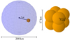 |
Fig. 1. Sketch of the ignition configuration. The blue sphere only serves to guide the eye. The enlarged figure shows the morphology of the ignition spark. |
Our standard initial model is inspired by the results of simulations of the simmering phase (Zingale et al. 2009). The central density ρc is set to 2.6 × 10⁹ g cm−3, the central temperature to 6 × 10⁸ K with an adiabatic decrease down to 1 × 10⁸ K, and constant afterwards. This temperature profile approximates the conditions during convective carbon burning prior to explosion and is thus better motivated from a physical point of view than the assumption of a cold isothermal WD. The actual effect, however, on the outcome of the simulation is small and should not be overestimated. The deflagration is ignited at an off-center radius of roff = 60 km, and, therefore, the model is named r60_d2.6_Z. The model name encodes the most important parameters, that is, the offset-radius in km (r), the central density in 109 g cm−3 (d), and the metallicity in units of the solar value Z⊙ (Z).
In this study, we varied roff between 10 km and 206 km, ρc between 1 and 6 × 10⁹ g cm−3 and the metallicity (only for the standard model) between 1 × 10⁻⁴ Z⊙ and 2 Z⊙. Since the WD is spherically symmetric, the location of the ignition spot can be chosen arbitrarily. We always placed the spark on the positive x-axis with x = roff and y, z = 0. A summary of the suite of models and results for the ejecta, that is, unbound material with Ekin > Egrav, can be found in Table A.1. With respect to the roff parameter we distinguish three groups in the set of models: (i) models that were ignited in the inner part of the star, that is, at 10 km. (ii) models in which the ignition is placed at around 60 km (standard model) always at the same mass coordinate, that is, roff = 45 − 82 km. (iii) models where the ignition kernel is located at around 150 km also always at the same mass coordinate, that is, roff = 114 − 206 km (see also Fig. 2).
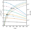 |
Fig. 2. Initial density profiles (solid lines), cumulative masses (dashed lines) and ignition radii indicated by scatter points. Solid squares depict that models with intermediate to high ignition radii are ignited at same mass coordinate. |
In addition, we have added two models of rigidly rotating WDs ignited at roff = 60 km with a central density of 2 × 10⁹ g cm−3. The ignition spark is located perpendicular to the rotation axis (z-axis) for the first model, r60_d2.0_Z_rot1 and directly on the rotation axis for the second, Model r60_d2.0_Z_rot2. Due to a more complex setup procedure of the initially rotating WD compared to the standard model the temperature in the rotating WDs is held constant at 5 × 10⁵ K. The rotation velocity is close to break-up velocity (Ω = 2.73 rad s−1) increasing the mass of the WD by about ∼6% to 1.438 M⊙. Moreover, we investigate a scenario with a carbon depleted core. In line with Lesaffre et al. (2006) and Ohlmann et al. (2014) the inner carbon mass fraction is reduced to 0.28 and joined smoothly with the outer regions (X(C) = 0.5) at a core mass of ∼1 M⊙. This model is labeled r60_d2.6_Z_c0.28.
5. Hydrodynamic simulations
The one-sided, single-spot ignition deflagration models of this work usually proceed as follows: The burnt fuel inside the hot bubble is lighter than its surroundings, and, thus, is subject to buoyancy. This is the reason why the flame cannot propagate against the density gradient and spreads to only one side of the WD. The deflagration itself is mediated by heat conduction, but the laminar burning speed of the flame is soon surpassed by the buoyant motion of the rising bubble. Subsequently, the burning becomes turbulent due to Rayleigh-Taylor and Kelvin-Helmholtz instabilities further increasing the fuel consumption. As soon as the turbulent flame reaches the outer parts of the WD, and, thus, lower densities, the burning quenches and the ashes flow around the star to collide at the far side. This is illustrated in Fig. 3.
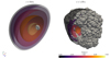 |
Fig. 3. Flame surface (gray) and isosurfaces of the density at ρ = 105, 106, 107, 108, 109 g cm−3 (see colorbar) for Model r60_d2.6_Z. Left panel: rising flame at t = 0.6 s while right panel: flame front when it has almost wrapped around the WD. We want to note, that the illustration is not to scale. In fact the WD has already expanded significantly in the right panel. |
The key outcomes of our parameter study are summarized in Table A.1 for ejected material and in Table A.2 for the WD remnant. We find 56Ni masses from 0.0058 to 0.092 M⊙ and ejected masses between 0.014 and 0.301 M⊙. It is interesting to note that the lowest as well as the highest 56Ni mass (the mass of 56Ni translates to the luminosity of the event and we therefore refer to bright and faint models when it comes to high or low 56Ni masses, respectively) are found in high-density models. The brightest model is r10_d4.0_Z and the faintest one is Model r114_d6.0_Z. Overall, this suite of models neither reaches the bright members of the SNe Iax subclass (SN 2005hk, SN 2011ay, SN 2012Z, etc.) nor the very faint explosions (SN 2008ha, SN 2010ae, SN 2019gsc). However, the 56Ni yield of our faintest model is only ∼1.9 times higher than the estimated value of 3 × 10⁻³ M⊙ for SN 2008ha (Foley et al. 2009). Furthermore, the brighter models of our sequence (r10_d4.0_Z, r10_d5.0_Z, r10_d6.0_Z) eject more 56Ni than the N3 model of F14 although only one ignition spark has been used. The 56Ni masses in this study and also in previous works are plotted against ejected mass in Fig. 4. Our models cover the low-energy end of the pure deflagration model distribution and show slight overlap with the F14 and J12 studies. Only the hybrid CONe WD model of K15 falls below the faintest model in the current study. Moreover, the new set of models extends the almost one-dimensional sequence in the M(56Ni)–Mej-plane. Despite varying initial conditions, that is, central densities and ignition configurations, and different codes employed, all models follow a linear relation between M(56Ni) and Mej to good approximation. However, it has been pointed out by K13 and K15 that an increase in Mej at a constant value of M(56Ni) is highly desirable to obtain broader light curves as observed in SNe Iax. The ratio of M(56Ni) to Mej is shown in Fig. 5. These values are comparable to those presented by F14 and show only little scatter. Therefore, it seems unlikely that SNe Iax can be explained by only one scenario taking into account results of the currently available pure deflagration models.
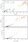 |
Fig. 4. Ejected 56Ni mass vs. Mej (upper panel), Mej vs. Enuc (middle panel) and Ekin, ej vs. Enuc (lower panel) for this work (black circles) and the works of J12, F14, K15 and L20. L12 only provide yields for IGEs, but not for 56Ni. To provide an approximate value for 56Ni, we multiplied the IGE masses with a factor of 0.7 in agreement with the MIGE to M(56Ni) ratios of L14 who use the same initial model. Measurements for M(56Ni) and Mej for SN 2002cx, 2008ha, 2012Z and were taken from McCully et al. (2014b), and references therein. Values for SN 2015H are from Magee et al. (2016) and for SN 2014ck from Tomasella et al. (2020). |
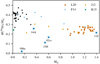 |
Fig. 5. Ejected mass vs. M(56Ni)/Mej for this work (black circles) and the works of J12, F14, K15, and L20. |
Since the new set of single-spot ignited models only covers the fainter and moderately bright members of the SN Iax class, we have relaxed the restriction of one ignition spark. We have recalculated Model N5 (5 ignition kernels) from F14 which has been compared to SN 2005hk by K13. The N5 ignition configuration has been combined with the initial condition of our standard model r60_d2.6_Z. We find that also with the updated version of the LEAFS code brighter SNe Iax can be reached. The new version of N5, Model N5_d2.6_Z, yields values of Enuc, M(56Ni), etc. (see Table A.1) slightly below those of the F14 version. This is due to the lower central density of 2.6 × 10⁹ g cm−3 compared to 2.9 × 10⁹ g cm−3 in the older run. The relations discussed above, however, do not change compared to the single-spot ignited models. Interestingly, Model N5_d2.6_Z is the brightest model in the current study with M(56Ni) = 0.136 M⊙ although Model r10_d6.0_Z releases more nuclear energy. The difference originates from the more neutron-rich nucleosynthesis at high densities reducing the amount of 56Ni in relation to stable IGEs (see also Sect. 5.1).
5.1. Dependence on central density
The influence of the central density on the nuclear energy release is twofold: (i) Assuming an identical ignition geometry, more mass is burned initially in the high-density case, and, thus, the energy production is higher in the early phase of the deflagration. (ii) Due to the steeper density gradient the effective gravitational acceleration is larger at high densities, and, thus, the buoyancy force acting on the low-density bubble increases. This speeds up the growth of Rayleigh-Taylor instabilities and also the transition from the laminar burning regime to turbulent burning (see also Röpke & Hillebrandt 2006). Moreover, a rather small effect might stem from the fact that the laminar burning velocity itself is higher for higher densities (Timmes & Woosley 1992). This increase of the burning rate at early times is, however, counteracted by the expansion of the WD. Since the flame is faster at high densities, the WD expands in a shorter period of time and the flame reaches the surface significantly earlier than for low densities. Hence, the burning is quenched earlier and limits the amount of burnt material. This competition between flame propagation and expansion of the WD is of particular importance for the energy release of the models presented in this study.
An increase in the ejected mass of 56Ni, that is, the brightness of the explosion, is also expected for higher densities. Since more material is burnt in total and especially at high densities more IGEs, and therefore also 56Ni, will be produced. The synthesis of 56Ni, however, does not increase linearly with the IGEs because of the neutron-rich environment due to an increasing rate of electron captures at high densities. If matter burns to NSE the neutron excess of the most abundant isotope is close to the neutron excess of the burning material, and, thus, the symmetric isotope 56Ni is not favored under these conditions (see Woosley et al. 1973, for instance).
To isolate the influence of the initial central density, we compare models ignited at a fixed radius, that is, the models ignited at roff = 10 km (r10_dXX_Z, see Table A.1). We observe a trend expected from theoretical considerations (see above): The nuclear energy release and the ejected masses increase from low (1 × 10⁹ g cm−3) to high (6 × 10⁹ g cm−3) central densities at ignition. Moreover, the value of M(56Ni) in models r10_d5.0_Z and r10_d6.0_Z is lower than in Model r10_d4.0_Z although the IGE yields are higher. This is due to higher electron capture rates at high density, and, therefore, more neutron-rich environment. This indicates that Model r10_d4.0_Z is close to the brightest explosion we can produce with a single-bubble ignition (models at higher roff are fainter, see Table A.1). The decreasing trend of M(56Ni)/MIGE is also present for all other ignition radii (see Table A.1). We find values of M(56Ni)/MIGE in the ejecta ranging from 0.88 at low central densities to 0.50 at high densities.
In summary, the flame evolves faster with increasing central density, and, thus, the energy released at early times rises. Therefore, the WD also starts to expand significantly earlier for higher central densities. However, the fast burning can always compensate for the expansion in models with fixed ignition radius (10 km) which leads to a monotonic increase of released nuclear energy with increasing central density.
5.2. Dependence on ignition radius
For a fixed central density, we observe the expected, decreasing trend in nuclear energy generation and ejected mass for increasing ignition radii (see Table A.1). This seems rather obvious because there is less mass available to burn for larger radii since the deflagration only propagates outward and not against the density gradient. However, the interplay between the flame velocity and the expansion of the WD (see Sect. 5.1) also is a significant factor here. We find that for all models except those with lowest density, that is, ρc = 1 × 10⁹ g cm−3, the total amount of burnt mass decreases for larger ignition radii. The volume of the flame during the burning phase (until t ∼ 2 s) is always largest for models ignited at large ignition radii reflecting the faster evolution of the flame due to the higher gravitational acceleration g (the maximum of g is only reached at r > 400 km). In contrast, the total mass burned, and with it the nuclear energy release, is higher for small ignition radii. This reflects that the average density at which material is burned makes up for the smaller volume filled by the flame in the first ∼2 s. Only in the case of Model r82_d1.0_Z, the increased flame velocity can overcompensate the expansion of the WD and leads to slightly higher nuclear energy release than for Model r10_d1.0_Z.
In the model sequences of intermediate and high ignition radii, that is, 45 to 82 km and 114 to 206 km, respectively, we have eliminated the difference in mass outside the ignition radius by igniting at the same mass coordinate (see also Fig. 2). For the reasons discussed above, the most energetic explosions in the intermediate sequence are those at low central density (r82_d1.0_Z and r65_d2.0_Z). Enuc increases again for the highest central densities (ρ = 5 − 6 × 10⁹ g cm−3). This indicates that the flame speed starts to compensate for the expansion in these models. In the models with large ignition radii the differences almost vanish and the trend in Enuc becomes monotonically decreasing. The lowest amount of 56Ni (M(56Ni) = 0.0058 M⊙), and, therefore, also the faintest explosion results from the model at highest central density and largest ignition radius, that is, Model r114_d6.0_Z. This is still a factor of ∼1.9 above the M(56Ni) mass inferred from observations of SN 2008ha (Foley et al. 2009), but the trends in this study suggest that such a low value could easily be reached by increasing the ignition radius even further. Moreover, the M(56Ni) to MIGE ratio does not drop off very significantly for increasing densities since a larger part of the inner core is left unburned for a large ignition radius.
We note that for models ejecting very little mass, that is, Mej ≲ 0.08 M⊙, the data show some scatter destroying monotonic trends. There is, in general, a decrease in M(56Ni) in the model sequence with large ignition radius from Model r206_d1.0_Z to r114_d6.0_Z which is interrupted by an unexpected increase from Model r163_d2.0_Z to r150_d2.6_Z, for instance. We are not able to explain this deviation by any physical properties of the respective explosion model. Instead, we suspect that the real differences between these models are too subtle to be captured by our simulations.
5.3. Dependence on metallicity
The net effect of metallicity is that it introduces a neutron excess (reduction of Ye) which has several effects on the explosion dynamics. First, the initial WD becomes more compact and lighter with increasing metallicity because the degenerate electron pressure decreases as Ye decreases. Second, the laminar flame speed is enhanced by the presence of 22Ne which is by far the most abundant species aside from C and O (Chamulak et al. 2007). This is, however, only important during the very early stages of the deflagration before turbulence introduced by Rayleigh-Taylor and Kelvin-Helmholtz instabilities governs the effective flame speed. Third, a neutron-rich environment leads to a decrease in the production of 56Ni in NSE (Timmes et al. 2003) since it favors the synthesis of more tightly bound, neutron-rich nuclei such as 57, 58Ni. Thus, the energy release is slightly higher for higher metallicity (Townsley et al. 2009). Finally, a reduction of Ye has only negligible influence on the buoyancy force (Townsley et al. 2009). On average, the effect of metallicity on the explosion dynamics is rather small. This is supported by Models r60_d2.6_XZ (X = 10−4, 10−3, 10−2, 10−1, 1, 2). They can be seen as identical regarding their values for Enuc, Mej, M(56Ni) since no real trend is visible in the data.
A decrease in M(56Ni) is expected for low metallicities which might again help in reducing the M(56Ni) to Mej ratio. This trend, however, is too subtle to be observed in this study and the small scatter is more likely to originate from numerical inaccuracies. The value of Ye in the high density regime of MCh explosions, in addition, is dominated by the effect of electron captures during the explosion whereas in sub-MCh models the initial metallicity is basically the only parameter determining the neutron excess. Nevertheless, the nucleosynthesis yields are expected to differ for varying metallicity. A detailed investigation of nucleosynthetic postprocessing data, however, is not the focus of this work. The nucleosynthesis yields of Model r60_d2.6_Z are included an analyzed in the work of Lach et al. (2020) labeled as Model R60. The model does produce a value of [Mn/Fe] = 0.11, and, thus, these explosions might play a role in the enrichment of the Universe with Mn in addition to helium shell detonations (Lach et al. 2020; Gronow et al. 2021) and various types of core collapse supernovae. The role of the latter is not a settled issue yet (compare the GCE studies of Prantzos et al. 2018; Kobayashi et al. 2020, for instance). The nucleosynthesis results of our parameter study will be published on HESMA (Kromer et al. 2017) for further use in GCE studies.
5.4. Rotating models
In the single degenerate scenario of SNe Ia the WD is not only expected to accrete mass from its donor star but also angular momentum (spin-up). This further stabilizes the WD against gravity and total masses highly exceeding MCh are possible (Yoon & Langer 2005). At some point, the material available for accretion might be exhausted and the accretion processes slows down or stops completely and a period of loss of angular momentum ensues (spin-down). During this spin-down the critical mass Mcrit of the WD decreases and a deflagration might be ignited as soon as it is exceeded by the WD mass. A rigidly rotating WD serves as a lower limit for Mcrit. This spin-up/spin-down scenario was proposed by Di Stefano et al. (2011).
Based on the work of Pfannes et al. (2010), we expect minor differences between the rigidly rotating models and the nonrotating model. On the one hand, more mass is available for burning (∼6%) in the rotating case which can lead to a higher nuclear energy release. On the other hand, the rotating WD progenitor is more tightly bound making it harder to eject material. Moreover, due to the shallower density gradient the relative fraction of IGEs compared to the total mass of the burning products decreases with increasing rotation velocity. These effects are even more prominent for fast, differentially rotating WDs (see also Fink et al. 2018). In addition, the propagation of the deflagration front is influenced by rotation. Since buoyancy is stronger parallel to the rotation axis due to the steeper density gradient and the flow vertical to the latter is suppressed because the material needs to gain angular momentum, the flame preferentially rises toward the poles. Therefore, the ignition conditions in this study have a large influence on the explosion compared to centrally distributed, multiple ignition sparks.
We compare the rotating models (Model r60_d2.0_Z_rot1 and r60_d2.0_Z_rot2) to Model r65_d2.0_Z. The minor difference in roff is not expected to obscure the differences originating from rotation. Table A.1 reveals that the outcome of the explosion indeed depends on the ignition location. The nonrotating model is bracketed by the rotating explosions in terms of Enuc, Mej, M(56Ni), MIGE, MIME and Ekin, ej. Model r60_d2.0_Z_rot1 yields higher values than Model r60_d2.0_Z_rot2 and is therefore expected to be brighter as well. The reason for this is that Model r60_d2.0_Z_rot2 is ignited on the rotation axis, and, thus, the flame spreads along this axis very fast and leads to a fast expansion of the star (see the discussion on expansion v.s. flame speed in Sect. 5.2). In Model r60_d2.0_Z_rot1 the deflagration is ignited perpendicular to the rotation axis which prevents burning directly toward the surface by the rotation and propagates toward north and south pole instead. The consequence of this is that the expansion is delayed, more material is burned and the explosion is more vigorous. However, these rigidly rotating models do not introduce any new characteristics in terms of their global properties to the model sequence. This indicates that rigidly rotating WDs as progenitor cannot add any diversity to our models for SNe Iax.
5.5. Carbon-depleted model
Another way to modify the progenitor is to vary its C/O ratio. The C mass fraction in the center of the WD is determined by the initial mass and metallicity of its zero-age main sequence progenitor and is expected to lie below 0.5 (Umeda et al. 1999; Domínguez et al. 2001). The value of X(C) is further reduced during convective carbon burning (simmering phase) while the outer layers accumulated via accretion and subsequent shell burning exhibit C/O ∼ 1 (Lesaffre et al. 2006). To investigate the effects of a reduced C mass fraction, we have calculated an explosion, Model r60_d2.6_Z_c0.28, set up with a C-depleted core (see Sect. 4) with a C mass fraction reduced to X(C) = 0.28. The total energy released during the explosion decreases with decreasing X(C) since the nuclear binding energy of O is higher than of C. This also decreases the buoyancy force and leads to a slower propagation of the flame. Therefore, Umeda et al. (1999) claim that higher X(C) leads to brighter SN events and Khokhlov (2000) and Gamezo et al. (2003) find that the burning in C depleted material is delayed. However, Röpke & Hillebrandt (2004) and Röpke et al. (2006b) examine the influence of the C/O ratio in 3D simulations and detect that its effect on the flame propagation is more subtle. In detail, the nuclear energy is buffered in α-particles when material is burned to NSE and only released in later stages of the explosion. This temporary storage of energy is enhanced for higher X(C) suppressing the buoyancy, and, thus, the propagation of the flame. Therefore, the C mass fraction does not affect the total production of IGEs significantly.
We corroborate this result with Model r60_d2.6_Z_c0.28 and find approximately the same total amount of IGEs and 56Ni as in the standard model r60_d2.6_Z (see Tables A.1 and A.2) although the nuclear energy released is lower for the C-depleted model. This, however, leads to less ejected mass in Model r60_d2.6_Z_c0.28. In contrast to the vigorously ignited models of Röpke et al. (2006b), the C/O ratio has an influence on the ejecta mass in sparsely ignited models. Since the relations between Mej, Enuc, MIGE and M(56Ni) do not show any deviations from the other models of the sequence (see Fig. 4) the carbon mass fraction is just another way to vary the brightness of the explosion but does not seem to help explaining the trends observed among SNe Iax.
5.6. Bound remnant
All models presented in this work are not energetic enough to unbind the WD completely. They leave behind massive bound remnants. These objects consist of a rather dense CO core and a puffed-up envelope of ashes admixed with CO material. This shell material is settling onto the WD core. If these stars manage to escape the binary system, for instance via a natal kick due to the asymmetric ignition, they can potentially be observed as chemically peculiar, high-velocity WDs. The first candidate for a SN Iax postgenitor, LP40–365, was observed by Vennes et al. (2017) and studied in more detail by Raddi et al. (2018a,b). Moreover, two more possible remnants of thermonuclear supernovae were discussed by Raddi et al. (2019). Although there are hints that these stars might be the product of a failed deflagration their origin is not completely established yet. Therefore, it is necessary to further investigate the long-term evolution of the bound remnant beyond 1D models (see Shen & Schwab 2017; Zhang et al. 2019) and also to obtain more detailed observations of such objects to shed light on their origin. Finally, a sound understanding of the structure and composition of the envelope is of vital importance since it may contribute to the light of the actual SN event (Kromer et al. 2013, 2015) and solve the problem of the fast decreasing light curve in current deflagration models. The 1D study of Shen & Schwab (2017) on this problem shows that a post-SN wind driven by the delayed decay of 56Ni in the envelope of the remnant contributes to the late-time bolometric light curve of the postgenitor. This contribution is in rough agreement with observed late-time light curves of SNe Iax.
Since the LEAFS code uses an expanding grid to track the ejecta the dense core is not very well resolved at the end of the simulations. Therefore, we can only provide some basic properties of the bound core directly after the explosion at t = 100 s (see Table A.2). First, all our models leave behind massive remnants in the mass range of 1.09 − 1.38 M⊙. These consist of a dense CO core (ρ ≳ 105 g cm−3) with a diameter of ∼4 × 109 cm and a large envelope polluted with burning products, that is, IGEs and IMEs (see Fig. 6). Unfortunately, we do not have postprocessing data for the remnant, and, hence cannot provide detailed nucleosynthesis results. From the hydrodynamic simulation we infer a mass fraction of 0.78 − 3.0% of IMEs and 4.2 − 10.1% of IGEs including 3.0 − 8.7% of 56Ni in the bound remnant. The amount of IGEs left inside the remnant is always larger than the amount of ejected IGEs except for the five most energetic explosion models. Moreover, the settling material is not well mixed showing alternating plumes of ash and fuel (see Fig. 6). The most noticeable feature is the prominent, cone-shaped region of unburned fuel at the left-hand side, that is, negative x-direction. This is exactly the opposite side of the ignition spark location and thus was not reached by the deflagration.
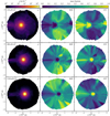 |
Fig. 6. Slices (x − y-plane) of density, IGE and CO mass fraction in the bound remnant for the bright model r10_5.0_Z (upper row) the moderately bright model r60_d2.6_Z (middle row) and the faint model r120_d5.0_Z (lower row). |
If we expect these peculiar WDs to be observed as single hyper-velocity runaway stars they need to escape the binary system via a natal kick, for example. While F14 report a maximum kick velocity of only 36 km s−1 J12 find velocities of up to 549 km s−1, which is sufficient to unbind the WD from its binary system. One possible explanation for this discrepancy was the monopole gravity solver employed by F14 which does not capture the full geometry of these asymmetric explosions. Here, we use an updated version of the LEAFS code accounting for self-gravity with an FFT gravity solver (see Sect. 3). We find kick velocities vkick, that is, the center of mass velocity of bound material, from 6.4 to 370 km s−1. Interestingly, vkick does not simply scale with explosion strength but is highest for low energetic models, decreases to around zero for intermediate ones and increases again for the most vigorous explosions (see Table A.2). Table A.2 also shows the kick velocity in x-direction vx. Since the flame is located off-center (positive x-direction in Fig. 6) and propagates outward, the WD is expected to receive a recoil momentum in the opposite direction, that is, the negative x-direction. This holds true for the most energetic explosions. The reason why the direction of the kick changes from negative to positive x-direction is hidden in the dynamical evolution of these kinds of explosions. In general, the one-sided ignition causes the flame to propagate to one direction only since a deflagration cannot proceed against the density gradient. In this case, the flame propagates to the right-hand side (positive x-direction, compare Figs. 6 and 7) until it reaches the surface of the WD and quenches. It then wraps around the star, the ashes eventually collide at the opposite side, and a strong flow is driven toward the inner regions. This flow then counteracts the initial momentum transferred by the flame propagation. The more vigorous the explosion the faster is the expansion of the WD and thus the ashes hardly collide at the far side of the star for our most energetic models. Therefore, the WD is pushed to the left (negative x-direction). For decreasing deflagrations strengths the momentum injected by the initial flame propagation drops and the star expands more slowly. Thus, the clash of the ashes at the antipode, and, subsequently, the inward flow of material becomes stronger until both effects balance each other and lead to almost zero kick velocity (intermediate models). In the case of our weaker explosions, the kick caused by the collision of the ashes dominates and leads to a push to the right-hand side (positive x-direction). The very faintest model in our parameter study, Model r114_d6.0_Z, breaks this trend and shows again a low kick velocity in the negative x-direction. Here, the total amount of mass brought to the surface by the deflagration has become too low to impact the momentum of the remnant. This shows that the final value of vkick strongly depends on the ignition geometry and the explosion strength. Finally, the remnant in Model N5_d2.6_Z receives a kick of 264.6 km s−1 which is significantly higher than 5.4 km s−1 reported by F14 employing a monopole gravity solver. This shows that the new solver has a large impact on the dynamics of these asymmetric explosion simulations.
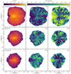 |
Fig. 7. Ejected material mapped to a velocity grid to serve as initial model for the RT. Shown are slices (x − y-plane) of density, 56Ni and CO mass fraction for the bright model r10_d5.0_Z (upper row) the moderately bright model r60_d2.6_Z (middle row) and the faint model r120_d5.0_Z (lower row). |
We emphasize that there is a large scatter in the values of vkick. The very coarse treatment of the inner parts of the WD at late times is most probably the reason for this, and, especially the differences in vkick for the models at different metallicity (r60_d2.6_Xz) lack an explanation since their energy release does not differ significantly. This suggests that the values can vary on the order of ∼100 km s−1 and can only serve as a rough estimate. However, the trend in vx explained above is not affected.
5.7. Ejecta
We have compiled slices through the ejecta of three representative models in Fig. 7 displaying the density, 56Ni mass fraction, and CO mass fraction, respectively. These models include r10_d5.0_Z (bright event, upper row), r60_d2.6_Z (intermediate brightness, middle row) and r120_d5.0_Z (faint event, lower row). Despite the asymmetric ignition, the ejecta in general appear spherically symmetric. Only for the bright model r10_d5.0_Z the material is skewed slightly to the side of the initial ignition (right-hand side in Fig. 7). This is due to the fact that the fast expansion prevents the ashes from wrapping around the core completely (see also Sect. 5.6). Moreover, it is also most apparent in r10_d5.0_Z that the opposite side of the ignition kernel is deficient in 56Ni (also burning products in general) which may introduce some viewing angle dependency in the synthetic spectra and light curves (see Sect. 6.3). This characteristic was also reported by J12. Apart from that, the ejecta are well-mixed (see also Fig. 9) showing a star-shaped pattern created by the Rayleigh-Taylor plumes. The rotating models, in contrast, show a more asymmetric structure (see Fig. 8). The ejecta in Model r60_d2.0_Z_rot1, for instance, are slightly shifted to the negative y-axis (left-hand side in Fig. 8). This is due to the angular momentum barrier (see Sect. 5.4) hindering the flame from sweeping around the WD as easily as in the nonrotating case. Model r60_d2.0_rot2, ignited on the rotation axis, is even more extreme concerning the asymmetry of the ejecta. The flame burns toward the north pole very quickly but is prevented from propagating around the core almost completely making the south pole deficient of burning products. Furthermore, the ejecta only reach velocities of ∼6000 km s−1 toward the south pole and ∼10 000 km s−1 at the north pole. This large-scale anisotropy might introduce significant viewing angle dependencies.
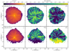 |
Fig. 8. Same as Fig. 7 (y − z-plane), but for the rotating Models r60_2.0_Z_rot1 (upper row) and r60_d2.0_Z_rot2 (lower row). |
To analyze the chemical composition of the ejecta we have compiled 1D average velocity profiles of the three reference models in Fig. 9. They show that the ejecta are mixed in the sense that IGEs, IMEs and unburned CO fuel are present at all velocities. However, we observe a weak decreasing trend for IGEs (including 56Ni) and IMEs toward high velocities and an increase in C and O. At the very edge of the ejecta, IGEs and 56Ni even begin to rise again. However, these trends are not as strong as predicted by Barna et al. (2018) and the increase of IGEs at very high velocities is in strong conflict with their work. Their abundance tomography study yields similar mass fractions for IMEs, IGEs and O in the inner regions but they find that C is virtually absent in the inner region and O dominates at high velocities. This comparison is, however, not too revealing since Barna et al. (2018) investigate the brightest members of the SN Iax subclass (SNe 2011ay, 2012Z, 2005hk, 2002cx) and our models represent faint and moderate members of the class. In a recent study, Barna et al. (2021) focus on the moderately bright SN Iax SN 2019muj (comparable to r10_d1.0_Z, r82_d1.0_Z, r65_d2.0_Z, r45_d6.0_Z in terms of M(56Ni)) and find no significant stratification except for carbon. Although their results are uncertain above ∼6500 km s−1 due to a sharp drop-off in density, they conclude that C is virtually absent below this value and steeply increases above in agreement with their earlier work (Barna et al. 2018) and in strong contrast to the models presented here. This conclusion, however, is not really strong since earlier spectra are needed to accurately model the outer layers of the ejecta. Apart from the case of C, a qualitative comparison of Figs. 9–11 in Barna et al. (2021) shows that our abundance profiles are concordant with their abundance tomography models showing a shallow decline of 56Ni and IMEs and an increase in the O mass fraction.
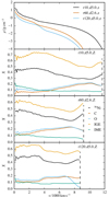 |
Fig. 9. 1D averaged density profile of the ejecta for Models r10_5.0_Z, r60_2.6_Z, r120_5.0_Z (upper panel). Lower three panels: 1D IGE, 56Ni, IME, C, and O profiles for the respective models. The dashed lines indicate a cutoff at densities below 10−4 g cm−3. |
6. Synthetic observables
To determine how the parameters varied in this study impact the synthetic observables, we carried out time-dependent 3D Monte-Carlo RT simulations using the ARTIS code (Sim 2007; Kromer & Sim 2009). Table A.3 lists the models for which RT simulations were carried out along with bolometric band, BVRI Bessel band, and ugriz Sloan band light curve parameters. We selected models that cover the range of 56Ni masses produced in the model sequence to explore its full diversity and investigate the impact of the varied parameters. For each RT simulation, 3 × 10⁷ energy packets were tracked through the ejecta for 150 logarithmically spaced time steps between 0.3 and 35 days post explosion. We use the atomic data set described by Gall et al. (2012). A gray approximation is used in cells that are optically thick (cf. Kromer & Sim 2009) and local thermal equilibrium (LTE) is assumed for times earlier than 0.4 days post explosion. Line of sight dependent light curves are calculated for 100 equal solid angle bins.
After the choice of initial conditions we make in the models (e.g., central density, ignition radius, metallicity, rigid rotation), we have a fully self-consistent modeling pipeline. This consists of the hydrodynamic explosion simulations, nucleosynthesis postprocessing step, and, finally, the RT simulations producing synthetic observables. This means we are comparing the predictions of our simulations, given a choice of initial parameters, to measured data. We are not providing any further input parameters (e.g., temperature, luminosity etc.) in order to fit the data and the comparisons we make should be interpreted within this context. Our self consistent pipeline also means it is important to take into account any assumptions made throughout our simulations. Of particular note for these models is the approximate non-LTE treatment of the ionization and excitation conditions in the plasma we adopt for our ARTIS RT simulations (see Kromer & Sim 2009 for more details). The non-LTE treatment of the ionization and excitation conditions in the plasma is an important ingredient in the modeling of SNe Ia (Dessart et al. 2014). No direct comparisons have been made between a MCh pure deflagration model simulated using approximate non-LTE and full non-LTE treatment in the regime that matches SNe Ia models. It is therefore uncertain how adopting a full non-LTE treatment for our models would change our results. However, previous works employing a full non-LTE treatment of the plasma conditions in models for SNe Ia (e.g., Blondin et al. 2013; Dessart et al. 2014; Shen et al. 2021) indicate that it will have noticeable effects on the synthetic observables produced on scales relevant for detailed comparisons to data. We are currently working on follow-up work in which we will re-simulate a subset of the models from the sequence presented here using the updated version of the ARTIS code developed by Shingles et al. (2020) which implements a full non-LTE treatment of the excitation and ionization conditions in the plasma. The results presented here will help prioritize models for further study.
6.1. Angle-averaged light curves
Our bolometric light curves are shown in Fig. 10. From this, it can be seen that the model light curves show a clear relationship between their bolometric evolution time scales and peak bolometric brightness, that is, the brighter models are slower in rise and decline. This is in agreement with the trend observed in the deflagration study of F14 driven by 56Ni synthesized in the explosion. In addition to this, the trends discussed in Sect. 5 for the choice of initial conditions and varied parameters, that is, ignition radius, central density, and metallicity, are confirmed by the results of the RT simulations: in general for a fixed central density the smaller the ignition radius of the model the brighter and broader its bolometric light curve will be. Additionally, for a fixed ignition radius the higher the central density the brighter and broader the model light curve. These trends, however, are not uniform for the whole model sequence and break down for the models with the highest central densities and also for those models which have both high central density and large ignition radius (see Sect. 5 for a more detailed discussion).
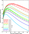 |
Fig. 10. Angle averaged bolometric light curves for a selection of our models. |
Figure 11 shows the BVRIgr band light curves for the selected models. Example SNe Iax are included for comparison. We emphasize that while we show observed SNe Iax for comparison here, the primary aim of this section is to comment on the overall light curve properties of the model sequence. In Sect. 6.4 we show a more detailed comparison to an observed SNe Iax. The estimated explosion epochs used for the observed SNe Iax 2005hk, 2012Z, 2019muj, 2008ha, and 2019gsc in Fig. 11 are taken from previous studies, specifically Phillips et al. (2007), Yamanaka et al. (2015), Barna et al. (2021), Valenti et al. (2009), and Srivastav et al. (2020), respectively. We note that this approach of comparing all light curves relative to literature values for explosion date may make the agreement of the model light curves with observed SNe Iax light curves seem relatively poor. However, if we allow the freedom to shift the explosion epochs of the observed SNe Iax later by even ∼2 days, (which is reasonable on the scale of the uncertainties in the estimated explosion epochs), significantly better agreement can be achieved between model and observed light curves, particularly for intermediate luminosity SNe Iax such as SN 2019muj (see Sect. 6.4 and Fig. 15).
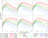 |
Fig. 11. Angle averaged BVRIgr band light curves for selected models. Observed light curves of the SNe Iax SN 2005hk (Phillips et al. 2007), SN 2012Z (Stritzinger et al. 2015), SN 2019muj (Barna et al. 2021), SN 2008ha (Foley et al. 2009) and SN 2019gsc (Srivastav et al. 2020; Tomasella et al. 2020) are included for comparison. |
From Fig. 11 it can be seen that the light curves show a similar relationship between their evolution timescales and peak magnitude in all bands as was observed for the bolometric light curves. Some models do show small variations in their band colors. However, these differences are relatively small and have little impact on the overall trends observed for the suite of models. Furthermore, any differences between models are too small to significantly impact the agreement between the models and observed SNe Iax.
The models show reasonably good agreement between their rise time scales and the data in both red and blue bands, although the red bands do appear to match the rise to peak of observed SNe Iax slightly better. However, the decline post peak of the data is matched much better by the models in the blue bands. The models are significantly too fast in the red bands to compare favorably with the light curve evolution of the data post peak (see also Figs. 14 and 17). This is similar to the trend observed previously in the deflagration study of F14. As noted above, when we move from brighter to fainter models in the sequence the models become faster in both rise and decline. This results in an evolution of the light curves of the fainter models that is significantly too fast to produce good agreement with the faintest members of the SN Iax class such as SN 2008ha and SN 2019gsc.
The choice of initial conditions leads to a variation in the 56Ni mass synthesized in the models and this is the characteristic which overwhelmingly controls the light curve properties of the models in terms of their absolute bolometric and band magnitudes and evolution time scales, regardless of what initial conditions are chosen. However, one parameter which leads to some variation in the light curve evolution is the 56Ni mass to ejecta mass ratio. The model with the lowest value of M(56Ni)/Mej, Model r48_d5.0_Z (see Tables A.1 and A.3, yellow dashed line in Figs. 10 and 11), is slightly slower in both rise and decline in the red bands than models with similar peak absolute band magnitudes (e.g., Model r60_d2.6_Z, green dash-dot line). While this does improve agreement between the model light curve evolution compared to the data in red bands (see r-band in Figs. 11 and 17) the red light curves for this model are not slowed down sufficiently to account for the slower light curve evolution of real SNe Iax.
6.2. Angle-averaged spectra
Figure 12 shows spectroscopic comparisons between a selection of models ranging from faintest (r114_d6.0_Z, blue) to brightest (r10_d4.0_Z, red) and three observed SNe Iax which span the diversity in brightness of the SNe Iax class. A variety of epochs from pre-peak to post-peak are chosen such that comparisons between the overall spectroscopic evolution of the model sequence and data can be made. As in Sect. 6.1 we note, that the purpose of this section is not to make detailed comparisons between the spectra of individual observed SNe Iax and the best agreeing model (see instead Sect. 6.4 for such a detailed comparison). Therefore, again for consistency, all times in Fig. 12 are relative to explosion with the same estimates for explosion epochs used for the data as referenced in Sect. 6.1.
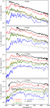 |
Fig. 12. Spectra over a variety of epochs for selected models which range from the bright to faint end of the model sequence alongside three observed SNe Iax: SN 2012Z (Stritzinger et al. 2015), one of the brighter members of the SN Iax class, SN 2019muj (Barna et al. 2021) which is an intermediate brightness SNe Iax, and SN 2019gsc (Srivastav et al. 2020) which is one of the faintest SNe Iax (see Figs. 13 and 17). The observed spectra shown here were obtained from WISeREP1 (Yaron & Gal-Yam 2012). All times are relative to explosion and in all cases real flux is plotted on a logarithmic scale. There is no data for SN 2019gsc 6 days after explosion and in the lowest panel the spectra were taken 23 days after explosion for SN 2012Z and SN 2019gsc. All observed spectra are flux calibrated to match the photometry and corrected for distance, red shift and reddening. |
From Fig. 12 we see that the bright and intermediate luminosity models show best spectroscopic agreement with the data in terms of their spectroscopic features for later epochs. The brightest model (r10_d4.0_Z, red) shows good agreement with one of the brighter SNe Iax, that is, SN 2012Z, for the latest epoch shown in terms of its spectroscopic features. In addition, the two intermediate luminosity models (r48_d5.0_Z, orange and r206_d1.0_Z, green) agree well with the intermediate luminosity SN Iax, that is, SN 2019muj, in terms of their spectroscopic features for all but the earliest epoch shown. However, while the bright and intermediate luminosity models match the slope and overall flux profile of observed SNe Iax spectra well at earlier epochs (at later times the flux agreement is poorer due to the model light curves evolving faster than the observed light curves), the synthetic spectra show too many distinct spectral features compared to the data at earlier times (6, 8, and 12 days after explosion for SN 2012Z and 6 days after explosion for SN 2019muj).
The faintest model (r114_d6.0_Z, blue) shows poor spectroscopic agreement with the faint SN Iax, SN 2019gsc. This model has spectra that have significantly too many spectral features compared to the data at all epochs. Therefore, the fainter models provide a much poorer match to the spectroscopic evolution of the data than the bright and intermediate luminosity models. From Fig. 12 it is also clear that Model r114_d6.0_Z is noticeably spectroscopically different to all the other models. This model has significantly more absorption in the blue region of the spectrum and more emission in the red wavelengths compared to the rest of the models which are more typical of the models in the sequence. This difference observed for Model r114_d6.0_Z is due to greater absorption by singly ionized IGEs such as iron, cobalt, nickel, and chromium in the blue region of the spectrum and subsequent re-emission in the red part of the spectrum. Since it is the faintest in the suite of models this characteristic can be attributed to this model having cooler ejecta which leads to a greater fraction of IGEs being in a lower ionization state.
Overall, we can see that all our models are spectroscopically very similar across all epochs, although the faintest model shows more noticeable differences. Therefore, the spectroscopic differences between models are much smaller than differences between models and data, although spectroscopic agreement between the models and data is reasonably good for bright and intermediate luminosity models particularly at later epochs. However, the poorer spectroscopic agreement at earlier times between models and data, even for the bright and moderate luminosity models shows there is disagreement in the early phase spectroscopic evolution of the models compared to data. This suggests that there are systematic differences in the spectroscopic evolution of the models and data which these simulations do not account for. We also note, that while the brightest model in our sequence does not quite reach the flux level of bright SNe Iax such as SN 2012Z, previous work by K13 and F14 has already shown that pure deflagration models are able to produce reasonable agreement with bright observed SNe Iax (although there are still some spectroscopic systematic differences). To confirm these findings still hold true when using the updated version of the LEAFS code we re-simulated the N5def model from K13 and F14 and simulated the RT using ARTIS. The results obtained are consistent with those reported by K13 and F14.
6.3. Viewing-angle dependencies
Figure 13 illustrates the viewing angle dependencies of the bolometric light curve properties (peak absolute bolometric magnitude, bolometric rise time to peak and bolometric decline post peak) for the selection of models for which RT simulations were carried out. In addition, Fig. 14 shows the viewing angle dependencies of B-band peak absolute magnitude and rise time for the selected models and includes observed SNe Iax for comparison. As can be seen from Figs. 13 and 14 the models occupy a one-dimensional sequence where the brighter the model the slower its rise to peak and decline post peak (the models of K13 and F14 also lie on this sequence). As discussed in Sect. 6.1 this trend is driven by the 56Ni mass synthesized in the models with secondary parameters having little impact on this overall trend. However, there can be variations of up to a magnitude at peak in both the bolometric and band light curves for certain models due to viewing angle effects, as well as significant variation in light curve evolution in both rise and decline. In particular, from Fig. 13 (right panel) we can see that there is a clear correlation between the peak bolometric brightness of the model viewing angles and their rate of decline: the brighter viewing angles have faster declining light curves post peak. An explanation for this is that the brighter viewing angles correspond to those in which there is a higher concentration of 56Ni near to the surface of the ejecta. Therefore the radiation due to the decay of this 56Ni will have to travel through less material to escape the ejecta leading to a faster evolution post peak.
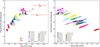 |
Fig. 13. Viewing angle dependencies of the bolometric light curveproperties for selected models. The solid circles represent the angle-averaged values and the crosses represent values from 100 different viewing angles for each model. The error bars depict the standard deviation of the viewing angle distribution for each model. Left panel: the peak bolometric-band magnitude is plotted against rise time. Alongside the models, estimates of peak bolometric magnitude and rise times for the observed SNe Iax SN 2019gsc (Srivastav et al. 2020, taking the values calculated for their full blackbody bolometric light curve), SN 2008ha (Foley et al. 2009), SN 2019muj (Barna et al. 2021), SN 2014ck (Tomasella et al. 2016), SN 2012Z (Yamanaka et al. 2015), SN 2005hk (Phillips et al. 2007), and SN 2009ku (Narayan et al. 2011) are included (represented by red markers and labeled by name). The different marker styles representing the SNe Iax of diamond, square, triangle, and plus correspond to SNe Iax where errors were quoted for both rise time and peak bolometric magnitude, only for peak bolometric magnitude, only for rise time and no errors quoted respectively. Where uncertainties were not quoted the uncertainties are still significant, particularly in rise times that can have uncertainties as much as several days. Right hand panel: peak bolometric-band magnitude vs. decline rate in terms of |

6.3.1. Viewing-angle dependencies of nonrotating models
The nonrotating model spectra do not show particularly strong viewing angle dependencies. The most noticeable effect is the velocity shifts of spectral lines: spectral features exhibit different blue shifts depending on the direction they are viewed from. The velocity shifts of spectral features can differ by up to ∼1000 km s−1. For all models the faint viewing angles have spectral features which are more blue shifted than for the bright viewing angles. Towards the blue wavelengths (less than ∼6000 Å) the bright models show less strong absorption than the faint models which is in better agreement with what is observed in the data (see Fig. 12). However, this effect is still too small to significantly improve the agreement of any of the individual models with the spectra of observed SNe Iax. Conversely, the red wavelengths show only very small differences in their flux when observed from different viewing angles. Variations in flux between different viewing angles can however lead to improved agreement with the overall flux of the spectra of an observed SNe Iax for selected viewing angles.
The nonrotating models also show some viewing angle dependencies in their light curves. Viewing-angles closer to the ignition spark (which is always on the positive x-axis for the nonrotating models) tend to be fainter, whereas those viewing angles further from the ignition spark tend to be the brightest. This is the case for all models for which RT simulations were carried out except the two faintest models in the sequence (r114_d6.0_Z and r120_d5.0_Z) which, by contrast, have brighter viewing angles closer to the ignition spark and fainter viewing angles further from the ignition spark. These two models have a noticeably different structure from the other models in the sequence (see r120_d5.0_Z compared to the other models shown in Fig. 7 that have structures more representative of the rest of the models in the sequence).
In general, it is clear that viewing angle effects are modest but noticeable even for well mixed pure deflagration models. These viewing angle effects, while unable to explain all the differences between our models and observed SNe Iax, are relevant on the scale of comparisons between observed SNe Iax and the models. This can clearly be seen from Fig. 14 where the variation of  observed for individual models is comparable to the differences in
  between observed SNe Iax, particularly for the brighter SNe Iax. In addition, the spread of
  values for the bright models due to viewing angle effects puts certain model viewing angles in better agreement with observed SNe Iax than the angle-averaged values for the models. Finally, we note that neither the models with different metallicity nor the carbon-depleted model show any noticeable differences in their viewing angle dependencies compared to the other models in the sequence.
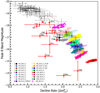 |
Fig. 14. B-band magnitude vs. |

6.3.2. Viewing-angle dependencies of rigidly rotating models
As discussed in Sect. 5.4 the rigidly rotating models are sensitive to whether the model is ignited perpendicular to the rotation axis (r60_d2.0_Z_rot1) or along the rotation axis (r60_d2.0_Z_rot2). The different choice of the ignition location in the rotational models leads to a variation in their brightnesses and produces a noticeably different ejecta structure for each model (see Fig. 8). The rigidly rotating models exhibit most significant differences with the nonrotating models in their viewing angle dependent spectra. Like the nonrotating models the rigidly rotating models show differences in their spectra depending on what line of sight they are viewed from, with the most noticeable differences in flux being seen in the blue wavelengths. Additionally, as was the case for the nonrotating models, the rigidly rotating models show spectral features which are more blue shifted for faint viewing angles and less blue shifted for bright viewing angles. However, the rigidly-rotating models show angle dependent differences between the blue shifts of their spectral features of over 2000 km s−1; double the difference in velocity shifts observed for the spectral features of the nonrotating models. The rigidly rotating models therefore exhibit significantly more asymmetry in their ejecta velocities compared to the nonrotating models. These models do not, however, show larger variations in their viewing angle dependent light curves compared to the nonrotating models.
6.4. Best agreeing model comparisons with SN 2019muj
In this section, we compare the intermediate luminosity SN Iax, SN 2019muj (Barna et al. 2021), with the model from our sequence in best agreement, to allow a more detailed comparisons between the light curves and spectra of one of our models and an observed SNe Iax. We have chosen SN 2019muj as it provides a good brightness match to the intermediate luminosity models in our sequence and also has good quality spectra to compare to (also including earlier epochs). Figure 15 shows the BVr light curves of SN 2019muj and the best agreeing model, r48_d5.0_Z. The angle-averaged as well as light curves for both a faint and bright viewing angle for this model are included. The model light curves are plotted relative to explosion time while we have shifted the band light curves of SN 2019muj such that their explosion epoch occurs 2 days later (MJD 58700) compared to the estimate from Barna et al. (2021) based on early light curve fitting, spectral fitting and bolometric light curve fitting (MJD 58697.5–58698.1). This means the B band peak of SN 2019muj matches the brightest viewing angle shown for Model r48_d5.0_Z (blue). Barna et al. (2021) do not include uncertainties in their estimates of the explosion epoch, however the first ATLAS detection of SN 2019muj is on MJD 58702.5 with only a marginal 1.8σ detection before this on MJD 58700.5. We therefore argue that shifting the explosion epoch 2 days later than what was estimated by Barna et al. (2021) is justified within the uncertainty of the explosion epoch of SN 2019muj. We have flux calibrated the spectra of SN 2019muj to match the photometry and corrected the light curves and spectra of SN 2019muj for redshift, reddening, and distance (taking the values estimated by Barna et al. 2021 of z = 0.007035, E(B − V) = 0.02, d = 34.1 Mpc and using Rv = 3.1). As discussed in Sect. 6.1, this model has the lowest value of M(56Ni)/Mej which results in it being slightly slower to rise and decline in the red bands compared to models with similar peak absolute band magnitudes. This leads to slightly better agreement with SN 2019muj. However, the improvement in agreement for the Model r48_d5.0_Z compared to other models of similar brightness (e.g., Models r10_d1.0_Z, r60_d2.0_Z_rot2, and r45_d6.0_Z) is small and the same conclusions are reached if we compare to one of these models instead.
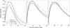 |
Fig. 15. BVr band light curves for Model r48_d5.0_Z (angle-averaged as well as a faint and bright viewing angle) compared with SN 2019muj (Barna et al. 2021). Model r48_d5.0_Z produces the best agreement in terms of its light curve and spectra compared to SN 2019muj. The model light curves are plotted relative to the explosion time predicted by our simulations, whereas the band light curves of SN 2019muj have all been shifted 2 days earlier than the explosion epoch estimated by Barna et al. (2021) such that SN 2019muj matches the brightest viewing angle shown (blue) for the model at B peak. The viewing angle looking along the axis that the ignition spark is placed is θ = 90° ϕ = 0° meaning the fainter viewing angle shown (red) is looking almost along this axis whereas the brighter viewing angle is looking along the axis directly opposite. |
Figure 15 demonstrates the importance of taking into account the viewing angle dependencies of our models. The brightest viewing angle shown (blue) has band light curves in noticeably better agreement with those of SN 2019muj than both the fainter viewing angle (red) and angle-averaged band light curves (green). Additionally, these brightest viewing angle band light curves are noticeably brighter than both the angle-averaged and faint viewing angle band light curves. This is especially true in B band where it is brighter than the angle averaged light curve by almost half a magnitude and more than this compared to the faint viewing angle shown. From Fig. 15 we see the brightest viewing angle shown for the r48_d5.0_Z model matches the rise to peak of SN 2019muj very well in all bands. Moreover, this viewing angle matches the decline of SN 2019muj well in all bands until approximately 5 days after B peak. Therefore, up until this time, this viewing angle provides a very good match to the colors of SN 2019muj. After this time, the decline of SN 2019muj is matched much better by the model in the B band than the V and particularly r band where the model light curves decline too quickly compared to those of SN 2019muj. As discussed in Sect. 6.1 (see also Sect. 6.5) this is a systematic discrepancy which effects all models in the sequence.
Figure 16 shows spectroscopic comparisons over a variety of epochs between SN 2019muj (black) and the viewing angle for Model r48_d5.0_Z in best agreement with SN 2019muj (blue in Fig. 15). From Fig. 16 we see that the model produces very good agreement in terms of the overall flux and spectral shape compared to SN 2019muj at all epochs apart from the latest epoch shown. For this latest epoch the model is too faint as we move to red wavelengths because the model declines faster than the data in the red bands at later epochs. The model is also able to successfully reproduce a significant proportion of the spectral features observed for SN 2019muj both in terms of their strength and location, although for the earliest epoch shown (4.2 days before B peak) the model does show slightly too many distinct spectral features compared to SN 2019muj (see also discussion in Sect. 6.2). We note that our synthetic spectra produce C features (at 4268, 4746, 6580, and 7234 Å) that are broadly consistent with observations of SN 2019muj (Barna et al. 2021). In particular, unlike the uniform composition model tested by Barna et al. (2021), we do not find the carbon features are significantly too strong at epochs around peak. Overall, from Figs. 15 and 16 it is clear that our models are able to reproduce many of the observed characteristics of the light curves, and, in particular, spectra of intermediate SNe Iax such as SN 2019muj very well, although some systematic differences remain.
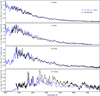 |
Fig. 16. Spectroscopic comparisons in absolute flux between SN 2019muj and the viewing angle for Model r48_d5.0_Z (blue in Fig. 15). Times are relative to B band maximum. |
6.5. Overall model sequence comparisons to observations
Figure 17 shows peak absolute r-band magnitude with rise time to r-peak (left panel) and decline rate post r-peak (right panel) for our models, models from the F14 and K15 studies as well as observed SNe Iax, and normal SNe Ia for comparison. From Fig. 17 we can see that our models map a significant portion of the wide variety of brightnesses covered by the SNe Iax class. They are, however, unable to reach the luminosities of the very brightest as well as the faintest SNe Iax. The new models extend the 1D sequence previously observed by F14 to more than a magnitude fainter at r-band peak and the new models appear to connect the F14 suite of models to the hybrid CONe models produced in the K15 study as an attempt to reach the faintest members of the Iax class (in particular SN 2008ha).
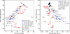 |
Fig. 17. Peak r-band magnitudes vs. rise time (left) and peak r-band magnitudes vs. decline rate in terms of Δm15 (right) for the models of F14 (green), our new sequence of models (blue), real SNe Iax (red) and normal SNe Ia (black). The filled red circles represent measurements in the r-band while the unfilled red circles represent measurements in the R-band. The observations include those compiled by Magee et al. (2016) as well as SN 2014ck (Tomasella et al. 2016), SN 2014ek (Li et al. 2018), SN 2018cxk (Yao et al. 2019), SN 2019muj (Barna et al. 2021), SN 2019gsc (Tomasella et al. 2020; Srivastav et al. 2020) and SN 2020kyg (Srivastav et al., in prep.). The blue diamond, cross and plus markers correspond to models which are variations on the standard r60_d2.6_Z model. The blue diamond represents r60_d2.6_Z_c0.28 (carbon depleted model), the cross depicts r60_d2.6_0.0001Z (reduced Z model) and the blue plus signs represent r60_d2.0_Z_rot1 and r60_d2.0_Z_rot2 (rigidly rotating models). The blue triangle represents the N5_d2.6_Z model from the F14 deflagration study simulated again using the updated version of the LEAFS code to quantify the difference caused by using the newer version of the code. The green star represents the hybrid CONe WD model produced by K15. |
It is interesting to note that single spark models from our model sequence are very similar to models from the F14 sequence of similar peak brightness both in terms of their light curve evolution (see Figs. 13, 14, and 17 where the N5_d2.6_Z model from the F14 sequence, re-simulated using the newest version of the LEAFS code, is included) and spectra. However, as expected, the single spark models do show greater viewing angle dependencies than the multi-spark models (see Figs. 13 and 14). This suggests that while using a multi-spark ignition is a physically improbable scenario there is relatively little signature of how the models were ignited in the synthetic observables they produce. This also provides some confirmation of the validity of the multispot ignition approach taken by J12, L14 and F14 to vary the strength of the deflagration in different models.
The 1D sequence followed by the models of previous works (see Sect. 2) and also our new model sequence is driven by the 56Ni mass synthesized in the explosion. Although the 56Ni mass to Mej ratio may have a small impact (see Sect. 6.1), no secondary parameters appear to have any dramatic impact on the overall behavior of the model sequence. Additionally, further changes to initial setups (such as models with different metallicity, the carbon-depleted model and rigidly rotating models) do not lead to any major break away from the general behavior of the model sequence with these different setups only being a further way in which the 56Ni synthesized in the explosions can be varied.
The sequence occupied by the models means they do not produce good agreement in their light curve evolution time scales, especially in their decline in the red bands (see Fig. 17) where the majority of the flux is observed. The agreement also becomes increasingly poor as we move to the faint models in our sequence because the models become faster in both rise and decline times for decreasing brightness. Faint SNe Iax, on the other hand, do not appear to evolve significantly faster than the brighter members of the SN Iax class (see Figs. 14 and 17). In addition, the model spectra show some systematic differences with observed SNe Iax, especially at early times and as we move to fainter models.
7. Conclusions
In this work we presented an extensive parameter study of 3D explosion simulations of deflagrations in MCh CO WDs. The aim of this research is to gain insights into the explosion mechanism of SNe Iax, a subluminous subclass of SNe Ia, since the pure deflagration scenario yields results in broad agreement with observations (Long et al. 2014; Fink et al. 2014; Kromer et al. 2013, 2015; Jordan et al. 2012). However, none of the studies carried out to date captures the full range in brightness and variations in decline rates and rise times, especially for the faint objects among this subclass. Moreover, multispot ignition was used as a tool to vary the explosion strength although the ignition in a single spark seems to be more realistic (Zingale et al. 2009, 2011; Nonaka et al. 2012). Therefore, we restricted the models to single-spot ignition and varied the location of the ignition spark from 10 to 206 km off from the center of the WD. We also employed central densities from 1 to 6 × 10⁹ g cm−3 and metallicities between 1 × 10⁻⁴ Z⊙ and 2 Z⊙. Finally, two rigidly rotating models and a progenitor with a carbon depleted core were added to the sequence to widen the parameter space and search for additional, physically motivated characteristics of a WD breaking the 1D trends found in previous studies.
We find that the sequence of models covers a large range in bolometric brightness ranging from −14.91 mag to −17.35 mag although the explosion is not controlled via the number of ignition bubbles. This demonstrates that single-spark ignition models can account for a wide range of luminosity as required to match the SN Iax observations. The faintest model is still about one order of magnitude brighter than the faint SN 2008ha and SN 2019gsc. However, a further reduction in brightness, that is, 56Ni mass, is rather easy to achieve by further increasing the ignition radius. On the other hand, it is hard to reach the brightest members of the SN Iax class with the restriction to a single spark ignition. Furthermore, we validate that, regardless of ignition, deflagrations do produce well mixed ejecta apart from some shallow abundance gradients. In addition, we report kick velocities of the bound explosion remnant of up to 369.8 km s−1 largely exceeding those reported by Fink et al. (2014). The kick velocity is, however, not a simple function of the deflagration strength. The direction of the natal kick changes by 180° for decreasing energy release leading to a minimum in the absolute value of the kick velocity.
Significant viewing angle effects in rise and decline times as well as variations of up to ∼1 mag in peak brightness further enhance the variations in observational properties. Additionally, both nonrotating and rigidly-rotating models show spectroscopic differences depending on the line of sight with variations in velocity shifts of ∼1000 km s−1 and ∼2000 km s−1 for the nonrotating and rotating models, respectively. Spectra, rise times and decline rates for the bright models of our sequence are in rough agreement with observations as already found by Fink et al. (2014) and Kromer et al. (2013). The intermediate luminosity models in our sequence also show reasonably good agreement. However, although the model observational properties show a significant diversity introduced by the wide exploration of the parameter space of the initial conditions and viewing angle effects, there are systematic differences between models and data which become increasingly apparent when moving to lower luminosities. For instance, the light curve decline is too fast in the red bands for all models, but as we move to the faint models this worsens and the overall light curve evolution also becomes too fast in all bands. The synthetic spectra of the faint models also show worse agreement across all epochs.
Overall, our findings suggest the pure deflagration scenario remains an appealing explanation for bright and intermediate luminosity SNe Iax. However, some systematic differences remain which need to be addressed. The work presented here, therefore leaves a few open questions. First, it needs to be investigated whether the decline of the model light curves can be slowed down within the framework of the MCh deflagration model. It seems that strong coupling between the ejected mass of 56Ni and the total ejected mass cannot be overcome easily by varying the parameters of our simulations. The most uncertain assumptions are the ignition conditions which need to be further investigated. Also the RT calculations introduce inaccuracies which need to be quantified and the effects of the new non-LTE version of ARTIS (Shingles et al. 2020) will be tested in future studies, which may help explain some of the systematic differences (particularly in spectral evolution) between models and observed SNe Iax. Another explanation for these systematic differences may be the properties of the models themselves: perhaps a more stratified ejecta structure as suggested by Stritzinger et al. (2015), Barna et al. (2017, 2018, 2021) may help match the spectral evolution of SNe Iax better. Moreover, we note our simulations do not take into account the possible impacts of the burning products in the bound remnant on the light curves and spectra. While this impact is very uncertain it has been suggested that the contribution of the burned material in the bound core may help to explain the long term evolution of SNe Iax light curves (Kromer et al. 2013; Foley et al. 2014; Shen & Schwab 2017) and their peculiar late time spectra (Foley et al. 2016). In addition, the effects due to the bound remnant could be increasingly relevant for the faint explosions, and, depending on the structure of the bound remnant, could contribute to SNe Iax light curves and spectra at earlier times (Kromer et al. 2015). A greater contribution of the remnant may be expected for fainter explosions as in fainter models the 56Ni mass in the bound remnant is predicted to be significantly higher than in the ejected material (e.g., Model r114_d6.0_Z has bound remnant 56Ni mass which is 5 times higher than the 56Ni mass in the ejected material). The bound remnant, therefore, may help explain some of the systematic differences between our models (particularly the fainter ones) and observed SNe Iax. However, as the impact, if any, of the burned material on top of the bound remnant on observed SNe Iax light curves and spectra is very uncertain future studies which better quantify the possible contribution of the bound remnant are key to understanding if this really can help explain some of the systematic differences between our models and observed SNe Iax.
The fact that the models can match some of the bright and intermediate luminosity events, but the observational trend does not naturally explain the faint explosions, may suggest that a different scenario might be at work. In particular, Valenti et al. (2009) argue that the most probable explanation for the very faint SN Iax supernova, SN 2008ha, is that it was produced in the low-energy core-collapse explosion of a hydrogen-deficient massive star. However, the fainter models in our sequence as well as the hybrid CONe deflagration model produced by Kromer et al. (2015) are able to reach luminosities approaching the low luminosities of the faintest SNe Iax such as SN 2008ha. In addition, while Valenti et al. (2009) argue there is a striking resemblance between SN 2008ha and the under-luminous type IIP SN 2005cs (Li et al. 2006; Pastorello et al. 2009) the comparisons they make between the early time spectra of SN 2008ha and those of SN 2002cx and SN 2005hk with their line velocities shifted by −3000 km s−1 show similarly good agreement. Moreover, speculations about ONe WD – neutron star mergers as a candidate for faint SNe Iax have been put forward by Bobrick et al. (2022). In summary, it seems likely that SNe Iax can be modeled by a combination of deflagrations in MCh WDs and other scenarios that may be needed to account for the fainter members of this class of transients.
Acknowledgments
This work was supported by the Deutsche Forschungsgemeinschaft (DFG, German Research Foundation) – Project-ID 138713538 – SFB 881 (“The Milky Way System”, subproject A10), by the ChETEC COST Action (CA16117), and by the National Science Foundation under Grant No. OISE-1927130 (IReNA). FL and FKR acknowledge support by the Klaus Tschira Foundation. FPC acknowledges an STFC studentship and SAS acknowledges funding from STFC Grant Ref: ST/P000312/1. NumPy and SciPy (Oliphant 2007), IPython (Pérez & Granger 2007), and Matplotlib (Hunter 2007) were used for data processing and plotting. The authors gratefully acknowledge the Gauss Centre for Supercomputing e.V. (www.gauss-centre.eu) for funding this project by providing computing time on the GCS Supercomputer JUWELS (Jülich Supercomputing Centre 2019) at Jülich Supercomputing Centre (JSC). Part of this work was performed using the Cambridge Service for Data Driven Discovery (CSD3), part of which is operated by the University of Cambridge Research Computing on behalf of the STFC DiRAC HPC Facility (www.dirac.ac.uk). The DiRAC component of CSD3 was funded by BEIS capital funding via STFC capital grants ST/P002307/1 and ST/R002452/1 and STFC operations grant ST/R00689X/1. DiRAC is part of the National e-Infrastructure. We thank James Gillanders for assisting with the flux calibrations of the observed spectra.
References
- Asplund, M., Grevesse, N., Sauval, A. J., & Scott, P. 2009, ARA&A, 47, 481 [NASA ADS] [CrossRef] [Google Scholar]
- Barna, B., Szalai, T., Kromer, M., et al. 2017, MNRAS, 471, 4865 [NASA ADS] [CrossRef] [Google Scholar]
- Barna, B., Szalai, T., Kerzendorf, W. E., et al. 2018, MNRAS, 480, 3609 [NASA ADS] [CrossRef] [Google Scholar]
- Barna, B., Szalai, T., Jha, S. W., et al. 2021, MNRAS, 501, 1078 [Google Scholar]
- Bauer, E. B., White, C. J., & Bildsten, L. 2019, ApJ, 887, 68 [Google Scholar]
- Blinnikov, S. I., & Khokhlov, A. M. 1986, Sov. Astron. Lett., 12, 131 [NASA ADS] [Google Scholar]
- Blondin, S., Dessart, L., Hillier, D. J., & Khokhlov, A. M. 2013, MNRAS, 429, 2127 [NASA ADS] [CrossRef] [Google Scholar]
- Bobrick, A., Zenati, Y., Perets, H. B., Davies, M. B., & Church, R. 2022, MNRAS, 510, 3758 [NASA ADS] [CrossRef] [Google Scholar]
- Brachwitz, F., Dean, D. J., Hix, W. R., et al. 2000, ApJ, 536, 934 [NASA ADS] [CrossRef] [Google Scholar]
- Branch, D., Fisher, A., & Nugent, P. 1993, AJ, 106, 2383 [NASA ADS] [CrossRef] [Google Scholar]
- Branch, D., Baron, E., Thomas, R. C., et al. 2004, PASP, 116, 903 [NASA ADS] [CrossRef] [Google Scholar]
- Branch, D., Dang, L. C., Hall, N., et al. 2006, PASP, 118, 560 [NASA ADS] [CrossRef] [Google Scholar]
- Bravo, E. 2019, A&A, 624, A139 [NASA ADS] [CrossRef] [EDP Sciences] [Google Scholar]
- Bravo, E., Gil-Pons, P., Gutiérrez, J. L., & Doherty, C. L. 2016, A&A, 589, A38 [NASA ADS] [CrossRef] [EDP Sciences] [Google Scholar]
- Bulla, M., Sim, S. A., & Kromer, M. 2015, MNRAS, 450, 967 [Google Scholar]
- Catalan, S., Ribas, I., Isern, J., & García-Berro, E. 2008, A&A, 477, 901 [NASA ADS] [CrossRef] [EDP Sciences] [Google Scholar]
- Chamulak, D. A., Brown, E. F., & Timmes, F. X. 2007, ApJ, 655, L93 [CrossRef] [Google Scholar]
- Chamulak, D. A., Brown, E. F., Timmes, F. X., & Dupczak, K. 2008, ApJ, 677, 160 [NASA ADS] [CrossRef] [Google Scholar]
- Chornock, R., Filippenko, A. V., Branch, D., et al. 2006, PASP, 118, 722 [NASA ADS] [CrossRef] [Google Scholar]
- Colella, P., & Woodward, P. R. 1984, J. Comput. Phys., 54, 174 [NASA ADS] [CrossRef] [Google Scholar]
- Denissenkov, P. A., Herwig, F., Truran, J. W., & Paxton, B. 2013, ApJ, 772, 37 [NASA ADS] [CrossRef] [Google Scholar]
- Denissenkov, P. A., Truran, J. W., Herwig, F., et al. 2015, MNRAS, 447, 2696 [NASA ADS] [CrossRef] [Google Scholar]
- Dessart, L., Hillier, D. J., Blondin, S., & Khokhlov, A. 2014, MNRAS, 441, 3249 [NASA ADS] [CrossRef] [Google Scholar]
- Di Stefano, R., Voss, R., & Claeys, J. S. W. 2011, ApJ, 738, L1 [Google Scholar]
- Domínguez, I., Höflich, P., & Straniero, O. 2001, ApJ, 557, 279 [CrossRef] [Google Scholar]
- Fernández, R., & Metzger, B. D. 2013, ApJ, 763, 108 [CrossRef] [Google Scholar]
- Fink, M., Kromer, M., Seitenzahl, I. R., et al. 2014, MNRAS, 438, 1762 [NASA ADS] [CrossRef] [Google Scholar]
- Fink, M., Kromer, M., Hillebrandt, W., et al. 2018, A&A, 618, A124 [NASA ADS] [CrossRef] [EDP Sciences] [Google Scholar]
- Foley, R. J., & Kirshner, R. P. 2013, ApJ, 769, L1 [NASA ADS] [CrossRef] [Google Scholar]
- Foley, R. J., Chornock, R., Filippenko, A. V., et al. 2009, AJ, 138, 376 [NASA ADS] [CrossRef] [Google Scholar]
- Foley, R. J., Challis, P. J., Chornock, R., et al. 2013, ApJ, 767, 57 [Google Scholar]
- Foley, R. J., McCully, C., Jha, S. W., et al. 2014, ApJ, 792, 29 [NASA ADS] [CrossRef] [Google Scholar]
- Foley, R. J., Jha, S. W., Pan, Y.-C., et al. 2016, MNRAS, 461, 433 [NASA ADS] [CrossRef] [Google Scholar]
- Fryxell, B. A., Müller, E., & Arnett, W. D. 1989, Hydrodynamics and Nuclear Burning, MPA Green Report 449 (Garching: Max-Planck-Institut für Astrophysik) [Google Scholar]
- Gall, E. E. E., Taubenberger, S., Kromer, M., et al. 2012, MNRAS, 427, 994 [NASA ADS] [CrossRef] [Google Scholar]
- Gamezo, V. N., Khokhlov, A. M., Oran, E. S., Chtchelkanova, A. Y., & Rosenberg, R. O. 2003, Science, 299, 77 [NASA ADS] [CrossRef] [Google Scholar]
- Gamezo, V. N., Khokhlov, A. M., & Oran, E. S. 2005, ApJ, 623, 337 [NASA ADS] [CrossRef] [Google Scholar]
- Gronow, S., Cote, B., Lach, F., et al. 2021, A&A, 656, A94 [NASA ADS] [CrossRef] [EDP Sciences] [Google Scholar]
- Hamuy, M., Phillips, M. M., Suntzeff, N. B., et al. 1996, AJ, 112, 2391 [Google Scholar]
- Hillebrandt, W., Kromer, M., Röpke, F. K., & Ruiter, A. J. 2013, Front. Phys., 8, 116 [Google Scholar]
- Hix, W. R., & Thielemann, F. 1999, ApJ, 511, 862 [NASA ADS] [CrossRef] [Google Scholar]
- Höflich, P., & Khokhlov, A. 1996, ApJ, 457, 500 [CrossRef] [Google Scholar]
- Hunter, J. D. 2007, Comput. Sci. Eng., 9, 90 [NASA ADS] [CrossRef] [Google Scholar]
- Iben, I., Jr., & Tutukov, A. V. 1984, ApJS, 54, 335 [NASA ADS] [CrossRef] [Google Scholar]
- Iwamoto, K., Brachwitz, F., Nomoto, K., et al. 1999, ApJS, 125, 439 [NASA ADS] [CrossRef] [Google Scholar]
- Jha, S. W. 2017, Handbook of Supernovae, 375 [CrossRef] [Google Scholar]
- Jha, S., Branch, D., Chornock, R., et al. 2006, AJ, 132, 189 [NASA ADS] [CrossRef] [Google Scholar]
- Jha, S., Riess, A. G., & Kirshner, R. P. 2007, ApJ, 659, 122 [NASA ADS] [CrossRef] [Google Scholar]
- Jordan, G. C., IV, Perets, H. B., Fisher, R. T., & van Rossum, D. R. 2012, ApJ, 761, L23 [NASA ADS] [CrossRef] [Google Scholar]
- Jülich Supercomputing Centre 2019, Journal of Large-scale Research Facilities, 5, A171 [Google Scholar]
- Kasen, D. 2006, ApJ, 649, 939 [NASA ADS] [CrossRef] [Google Scholar]
- Kashyap, R., Haque, T., Lorén-Aguilar, P., García-Berro, E., & Fisher, R. 2018, ApJ, 869, 140 [NASA ADS] [CrossRef] [Google Scholar]
- Kawabata, M., Kawabata, K. S., Maeda, K., et al. 2018, PASJ, 70, 111 [NASA ADS] [CrossRef] [Google Scholar]
- Kawabata, M., Maeda, K., Yamanaka, M., et al. 2021, PASJ, 73, 1295 [NASA ADS] [CrossRef] [Google Scholar]
- Khokhlov, A. M. 1989, MNRAS, 239, 785 [NASA ADS] [Google Scholar]
- Khokhlov, A. M. 1991, A&A, 245, 114 [NASA ADS] [Google Scholar]
- Khokhlov, A. M. 2000, ArXiv e-prints [arXiv:astro-ph/0008463] [Google Scholar]
- Kobayashi, C., Umeda, H., Nomoto, K., Tominaga, N., & Ohkubo, T. 2006, ApJ, 653, 1145 [NASA ADS] [CrossRef] [Google Scholar]
- Kobayashi, C., Leung, S.-C., & Nomoto, K. 2020, ApJ, 895, 138 [CrossRef] [Google Scholar]
- Kromer, M., & Sim, S. A. 2009, MNRAS, 398, 1809 [Google Scholar]
- Kromer, M., Fink, M., Stanishev, V., et al. 2013, MNRAS, 429, 2287 [NASA ADS] [CrossRef] [Google Scholar]
- Kromer, M., Ohlmann, S. T., Pakmor, R., et al. 2015, MNRAS, 450, 3045 [NASA ADS] [CrossRef] [Google Scholar]
- Kromer, M., Ohlmann, S. T., & Roepke, F. K. 2017, Mem. Soc. Astron. It., 88, 312 [Google Scholar]
- Kuhlen, M., Woosley, S. E., & Glatzmaier, G. A. 2006, ApJ, 640, 407 [NASA ADS] [CrossRef] [Google Scholar]
- Lach, F., Röpke, F. K., Seitenzahl, I. R., et al. 2020, A&A, 644, A118 [NASA ADS] [CrossRef] [EDP Sciences] [Google Scholar]
- Langanke, K., & Martínez-Pinedo, G. 2001, At. Data Nucl. Data Tables, 79, 1 [NASA ADS] [CrossRef] [Google Scholar]
- Lesaffre, P., Han, Z., Tout, C. A., Podsiadlowski, P., & Martin, R. G. 2006, MNRAS, 368, 187 [NASA ADS] [CrossRef] [Google Scholar]
- Leung, S.-C., & Nomoto, K. 2020, ApJ, 900, 54 [NASA ADS] [CrossRef] [Google Scholar]
- Li, W., Filippenko, A. V., Chornock, R., et al. 2003, PASP, 115, 453 [Google Scholar]
- Li, W., Van Dyk, S. D., Filippenko, A. V., et al. 2006, ApJ, 641, 1060 [NASA ADS] [CrossRef] [Google Scholar]
- Li, W., Leaman, J., Chornock, R., et al. 2011, MNRAS, 412, 1441 [NASA ADS] [CrossRef] [Google Scholar]
- Li, L., Wang, X., Zhang, J., et al. 2018, MNRAS, 478, 4575 [NASA ADS] [CrossRef] [Google Scholar]
- Liu, Z.-W., Kromer, M., Fink, M., et al. 2013, ApJ, 778, 121 [NASA ADS] [CrossRef] [Google Scholar]
- Livio, M., & Mazzali, P. 2018, Phys. Rep., 736, 1 [Google Scholar]
- Long, M., Jordan, G. C., IV, Van Rossum, D. R., et al. 2014, ApJ, 789, 103 [NASA ADS] [CrossRef] [Google Scholar]
- Lundqvist, P., Mattila, S., Sollerman, J., et al. 2013, MNRAS, 435, 329 [NASA ADS] [CrossRef] [Google Scholar]
- Lyman, J., Taddia, F., Stritzinger, M., et al. 2018, MNRAS, 473, 1359 [NASA ADS] [CrossRef] [Google Scholar]
- Magee, M. R., Kotak, R., Sim, S. A., et al. 2016, A&A, 589, A89 [NASA ADS] [CrossRef] [EDP Sciences] [Google Scholar]
- Magee, M., Sim, S., Kotak, R., Maguire, K., & Boyle, A. 2019, A&A, 622, A102 [NASA ADS] [CrossRef] [EDP Sciences] [Google Scholar]
- Marquardt, K. S., Sim, S. A., Ruiter, A. J., et al. 2015, A&A, 580, A118 [NASA ADS] [CrossRef] [EDP Sciences] [Google Scholar]
- McClelland, C. M., Garnavich, P. M., Galbany, L., et al. 2010, ApJ, 720, 704 [NASA ADS] [CrossRef] [Google Scholar]
- McCully, C., Jha, S. W., Foley, R. J., et al. 2014a, Nature, 512, 54 [NASA ADS] [CrossRef] [Google Scholar]
- McCully, C., Jha, S. W., Foley, R. J., et al. 2014b, ApJ, 786, 134 [NASA ADS] [CrossRef] [Google Scholar]
- McCully, C., Jha, S. W., Scalzo, R. A., et al. 2022, ApJ, 925, 138 [NASA ADS] [CrossRef] [Google Scholar]
- Narayan, G., Foley, R. J., Berger, E., et al. 2011, ApJ, 731, L11 [NASA ADS] [CrossRef] [Google Scholar]
- Neunteufel, P. 2020, A&A, 641, A52 [EDP Sciences] [Google Scholar]
- Nomoto, K., Kobayashi, C., & Tominaga, N. 2013, ARA&A, 51, 457 [CrossRef] [Google Scholar]
- Nonaka, A., Aspden, A. J., Zingale, M., et al. 2012, ApJ, 745, 73 [NASA ADS] [CrossRef] [Google Scholar]
- Ohlmann, S. T., Kromer, M., Fink, M., et al. 2014, A&A, 572, A57 [NASA ADS] [CrossRef] [EDP Sciences] [Google Scholar]
- Oliphant, T. E. 2007, Comput. Sci. Eng., 9, 10 [NASA ADS] [CrossRef] [Google Scholar]
- Osher, S., & Sethian, J. A. 1988, J. Comput. Phys., 79, 12 [NASA ADS] [CrossRef] [Google Scholar]
- Oskinova, L. M., Gvaramadze, V. V., Gräfener, G., Langer, N., & Todt, H. 2020, A&A, 644, L8 [NASA ADS] [CrossRef] [EDP Sciences] [Google Scholar]
- Pakmor, R., Röpke, F. K., Weiss, A., & Hillebrandt, W. 2008, A&A, 489, 943 [NASA ADS] [CrossRef] [EDP Sciences] [Google Scholar]
- Pakmor, R., Edelmann, P., Röpke, F. K., & Hillebrandt, W. 2012, MNRAS, 424, 2222 [Google Scholar]
- Pastorello, A., Valenti, S., Zampieri, L., et al. 2009, MNRAS, 394, 2266 [Google Scholar]
- Pérez, F., & Granger, B. E. 2007, Comput. Sci. Eng., 9, 21 [Google Scholar]
- Perlmutter, S., Aldering, G., Goldhaber, G., et al. 1999, ApJ, 517, 565 [Google Scholar]
- Pfannes, J. M. M., Niemeyer, J. C., Schmidt, W., & Klingenberg, C. 2010, A&A, 509, A74 [NASA ADS] [CrossRef] [EDP Sciences] [Google Scholar]
- Phillips, M. M. 1993, ApJ, 413, L105 [Google Scholar]
- Phillips, M. M., Li, W., Frieman, J. A., et al. 2007, PASP, 119, 360 [CrossRef] [Google Scholar]
- Piro, A. L., & Bildsten, L. 2008, ApJ, 673, 1009 [NASA ADS] [CrossRef] [Google Scholar]
- Prantzos, N., Abia, C., Limongi, M., Chieffi, A., & Cristallo, S. 2018, MNRAS, 476, 3432 [Google Scholar]
- Provencal, J. L., Shipman, H., Høg, E., & Thejll, P. 1998, ApJ, 494, 759 [NASA ADS] [CrossRef] [Google Scholar]
- Raddi, R., Hollands, M., Koester, D., et al. 2018a, ApJ, 858, 3 [NASA ADS] [CrossRef] [Google Scholar]
- Raddi, R., Hollands, M., Gänsicke, B., et al. 2018b, MNRAS, 479, L96 [NASA ADS] [CrossRef] [Google Scholar]
- Raddi, R., Hollands, M., Koester, D., et al. 2019, MNRAS, 489, 1489 [NASA ADS] [CrossRef] [Google Scholar]
- Rauscher, T., & Thielemann, F.-K. 2000, At. Data Nucl. Data Tables, 75, 1 [Google Scholar]
- Reinecke, M., Hillebrandt, W., & Niemeyer, J. C. 1999a, A&A, 347, 739 [NASA ADS] [Google Scholar]
- Reinecke, M., Hillebrandt, W., Niemeyer, J. C., Klein, R., & Gröbl, A. 1999b, A&A, 347, 724 [NASA ADS] [Google Scholar]
- Riess, A. G., Press, W. H., & Kirshner, R. P. 1996, ApJ, 473, 88 [Google Scholar]
- Ritter, A., Parker, Q., Lykou, F., et al. 2021, ApJ, 918, L33 [NASA ADS] [CrossRef] [Google Scholar]
- Röpke, F. K. 2005, A&A, 432, 969 [NASA ADS] [CrossRef] [EDP Sciences] [Google Scholar]
- Röpke, F. K. 2007, ApJ, 668, 1103 [CrossRef] [Google Scholar]
- Röpke, F. K., & Hillebrandt, W. 2004, A&A, 420, L1 [NASA ADS] [CrossRef] [EDP Sciences] [Google Scholar]
- Röpke, F. K., & Hillebrandt, W. 2005, A&A, 431, 635 [NASA ADS] [CrossRef] [EDP Sciences] [Google Scholar]
- Röpke, F. K., & Hillebrandt, W. 2006, in Origin of Matter and Evolution of Galaxies, eds. S. Kubono, W. Aoki, T. Kajino, T. Motobayashi, & K. Nomoto, AIP Conf. Ser., 847, 190 [Google Scholar]
- Röpke, F. K., & Sim, S. A. 2018, Space Sci. Rev., 214, 72 [Google Scholar]
- Röpke, F. K., Hillebrandt, W., Niemeyer, J. C., & Woosley, S. E. 2006a, A&A, 448, 1 [NASA ADS] [CrossRef] [EDP Sciences] [Google Scholar]
- Röpke, F. K., Gieseler, M., Reinecke, M., Travaglio, C., & Hillebrandt, W. 2006b, A&A, 453, 203 [NASA ADS] [CrossRef] [EDP Sciences] [Google Scholar]
- Röpke, F. K., Hillebrandt, W., Schmidt, W., et al. 2007, ApJ, 668, 1132 [NASA ADS] [CrossRef] [Google Scholar]
- Schmidt, B. P., Suntzeff, N. B., Phillips, M. M., et al. 1998, ApJ, 507, 46 [NASA ADS] [CrossRef] [Google Scholar]
- Seitenzahl, I. R., Townsley, D. M., Peng, F., & Truran, J. W. 2009, At. Data Nucl. Data Tables, 95, 96 [NASA ADS] [CrossRef] [Google Scholar]
- Seitenzahl, I. R., Ciaraldi-Schoolmann, F., Röpke, F. K., et al. 2013, MNRAS, 429, 1156 [NASA ADS] [CrossRef] [Google Scholar]
- Shen, K. J., & Schwab, J. 2017, ApJ, 834, 180 [NASA ADS] [CrossRef] [Google Scholar]
- Shen, K. J., Blondin, S., Kasen, D., et al. 2021, ApJ, 909, L18 [NASA ADS] [CrossRef] [Google Scholar]
- Shingles, L. J., Sim, S. A., Kromer, M., et al. 2020, MNRAS, 492, 2029 [NASA ADS] [CrossRef] [Google Scholar]
- Sim, S. A. 2007, MNRAS, 375, 154 [NASA ADS] [CrossRef] [Google Scholar]
- Soker, N. 2019, New Astron. Rev., 87, 101535 [CrossRef] [Google Scholar]
- Srivastav, S., Smartt, S. J., Leloudas, G., et al. 2020, ApJ, 892, L24 [NASA ADS] [CrossRef] [Google Scholar]
- Stritzinger, M. D., Hsiao, E., Valenti, S., et al. 2014, A&A, 561, A146 [NASA ADS] [CrossRef] [EDP Sciences] [Google Scholar]
- Stritzinger, M. D., Valenti, S., Hoeflich, P., et al. 2015, A&A, 573, A2 [NASA ADS] [CrossRef] [EDP Sciences] [Google Scholar]
- Taubenberger, S. 2017, Handbook of Supernovae, 317 [CrossRef] [Google Scholar]
- Thielemann, F.-K., Nomoto, K., & Hashimoto, M.-A. 1996, ApJ, 460, 408 [NASA ADS] [CrossRef] [Google Scholar]
- Thielemann, F.-K., Isern, J., Perego, A., & von Ballmoos, P. 2018, Space Sci. Rev., 214, 62 [CrossRef] [Google Scholar]
- Timmes, F. X., & Arnett, D. 1999, ApJS, 125, 277 [Google Scholar]
- Timmes, F. X., & Woosley, S. E. 1992, ApJ, 396, 649 [NASA ADS] [CrossRef] [Google Scholar]
- Timmes, F. X., Brown, E. F., & Truran, J. W. 2003, ApJ, 590, L83 [Google Scholar]
- Tomasella, L., Cappellaro, E., Benetti, S., et al. 2016, MNRAS, 459, 1018 [NASA ADS] [CrossRef] [Google Scholar]
- Tomasella, L., Stritzinger, M., Benetti, S., et al. 2020, MNRAS, 496, 1132 [NASA ADS] [CrossRef] [Google Scholar]
- Townsley, D. M., Jackson, A. P., Calder, A. C., et al. 2009, ApJ, 701, 1582 [NASA ADS] [CrossRef] [Google Scholar]
- Travaglio, C., Hillebrandt, W., Reinecke, M., & Thielemann, F.-K. 2004, A&A, 425, 1029 [NASA ADS] [CrossRef] [EDP Sciences] [Google Scholar]
- Umeda, H., Nomoto, K., Kobayashi, C., Hachisu, I., & Kato, M. 1999, ApJ, 522, L43 [NASA ADS] [CrossRef] [Google Scholar]
- Valenti, S., Pastorello, A., Cappellaro, E., et al. 2009, Nature, 459, 674 [NASA ADS] [CrossRef] [Google Scholar]
- Vennes, S., Nemeth, P., Kawka, A., et al. 2017, Science, 357, 680 [Google Scholar]
- Wang, B., & Han, Z. 2012, New Astron. Rev., 56, 122 [CrossRef] [Google Scholar]
- Whelan, J., & Iben, I. J. 1973, ApJ, 186, 1007 [Google Scholar]
- White, C. J., Kasliwal, M. M., Nugent, P. E., et al. 2015, ApJ, 799, 52 [NASA ADS] [CrossRef] [Google Scholar]
- Woosley, S. E., Arnett, W. D., & Clayton, D. D. 1973, ApJS, 26, 231 [NASA ADS] [CrossRef] [Google Scholar]
- Yamanaka, M., Maeda, K., Kawabata, K. S., et al. 2015, ApJ, 806, 191 [NASA ADS] [CrossRef] [Google Scholar]
- Yao, Y., Miller, A. A., Kulkarni, S. R., et al. 2019, ApJ, 886, 152 [NASA ADS] [CrossRef] [Google Scholar]
- Yaron, O., & Gal-Yam, A. 2012, PASP, 124, 668 [Google Scholar]
- Yoon, S., & Langer, N. 2005, A&A, 435, 967 [NASA ADS] [CrossRef] [EDP Sciences] [Google Scholar]
- Zeng, Y., Liu, Z.-W., & Han, Z. 2020, ApJ, 898, 12 [NASA ADS] [CrossRef] [Google Scholar]
- Zhang, M., Fuller, J., Schwab, J., & Foley, R. J. 2019, ApJ, 872, 29 [Google Scholar]
- Zhou, P., Leung, S.-C., Li, Z., et al. 2021, ApJ, 908, 31 [NASA ADS] [CrossRef] [Google Scholar]
- Zingale, M., Almgren, A. S., Bell, J. B., Nonaka, A., & Woosley, S. E. 2009, ApJ, 704, 196 [NASA ADS] [CrossRef] [Google Scholar]
- Zingale, M., Nonaka, A., Almgren, A. S., et al. 2011, ApJ, 740, 8 [NASA ADS] [CrossRef] [Google Scholar]
Appendix A: Simulation summary tables
Summary of the main properties of the ejected material and the initial conditions.
Main properties of the bound remnant and the respective initial conditions.
Angle averaged light curve properties for bolometric band and BVRI Bessel bands (top) as well as ugriz Sloan bands (bottom) for the selection of models for which RT simulations were carried out.
All Tables
Summary of the main properties of the ejected material and the initial conditions.
Angle averaged light curve properties for bolometric band and BVRI Bessel bands (top) as well as ugriz Sloan bands (bottom) for the selection of models for which RT simulations were carried out.
All Figures
|
Fig. 1. Sketch of the ignition configuration. The blue sphere only serves to guide the eye. The enlarged figure shows the morphology of the ignition spark. |
| In the text | |
|
Fig. 2. Initial density profiles (solid lines), cumulative masses (dashed lines) and ignition radii indicated by scatter points. Solid squares depict that models with intermediate to high ignition radii are ignited at same mass coordinate. |
| In the text | |
|
Fig. 3. Flame surface (gray) and isosurfaces of the density at ρ = 105, 106, 107, 108, 109 g cm−3 (see colorbar) for Model r60_d2.6_Z. Left panel: rising flame at t = 0.6 s while right panel: flame front when it has almost wrapped around the WD. We want to note, that the illustration is not to scale. In fact the WD has already expanded significantly in the right panel. |
| In the text | |
|
Fig. 4. Ejected 56Ni mass vs. Mej (upper panel), Mej vs. Enuc (middle panel) and Ekin, ej vs. Enuc (lower panel) for this work (black circles) and the works of J12, F14, K15 and L20. L12 only provide yields for IGEs, but not for 56Ni. To provide an approximate value for 56Ni, we multiplied the IGE masses with a factor of 0.7 in agreement with the MIGE to M(56Ni) ratios of L14 who use the same initial model. Measurements for M(56Ni) and Mej for SN 2002cx, 2008ha, 2012Z and were taken from McCully et al. (2014b), and references therein. Values for SN 2015H are from Magee et al. (2016) and for SN 2014ck from Tomasella et al. (2020). |
| In the text | |
|
Fig. 5. Ejected mass vs. M(56Ni)/Mej for this work (black circles) and the works of J12, F14, K15, and L20. |
| In the text | |
|
Fig. 6. Slices (x − y-plane) of density, IGE and CO mass fraction in the bound remnant for the bright model r10_5.0_Z (upper row) the moderately bright model r60_d2.6_Z (middle row) and the faint model r120_d5.0_Z (lower row). |
| In the text | |
|
Fig. 7. Ejected material mapped to a velocity grid to serve as initial model for the RT. Shown are slices (x − y-plane) of density, 56Ni and CO mass fraction for the bright model r10_d5.0_Z (upper row) the moderately bright model r60_d2.6_Z (middle row) and the faint model r120_d5.0_Z (lower row). |
| In the text | |
|
Fig. 8. Same as Fig. 7 (y − z-plane), but for the rotating Models r60_2.0_Z_rot1 (upper row) and r60_d2.0_Z_rot2 (lower row). |
| In the text | |
|
Fig. 9. 1D averaged density profile of the ejecta for Models r10_5.0_Z, r60_2.6_Z, r120_5.0_Z (upper panel). Lower three panels: 1D IGE, 56Ni, IME, C, and O profiles for the respective models. The dashed lines indicate a cutoff at densities below 10−4 g cm−3. |
| In the text | |
|
Fig. 10. Angle averaged bolometric light curves for a selection of our models. |
| In the text | |
|
Fig. 11. Angle averaged BVRIgr band light curves for selected models. Observed light curves of the SNe Iax SN 2005hk (Phillips et al. 2007), SN 2012Z (Stritzinger et al. 2015), SN 2019muj (Barna et al. 2021), SN 2008ha (Foley et al. 2009) and SN 2019gsc (Srivastav et al. 2020; Tomasella et al. 2020) are included for comparison. |
| In the text | |
|
Fig. 12. Spectra over a variety of epochs for selected models which range from the bright to faint end of the model sequence alongside three observed SNe Iax: SN 2012Z (Stritzinger et al. 2015), one of the brighter members of the SN Iax class, SN 2019muj (Barna et al. 2021) which is an intermediate brightness SNe Iax, and SN 2019gsc (Srivastav et al. 2020) which is one of the faintest SNe Iax (see Figs. 13 and 17). The observed spectra shown here were obtained from WISeREP1 (Yaron & Gal-Yam 2012). All times are relative to explosion and in all cases real flux is plotted on a logarithmic scale. There is no data for SN 2019gsc 6 days after explosion and in the lowest panel the spectra were taken 23 days after explosion for SN 2012Z and SN 2019gsc. All observed spectra are flux calibrated to match the photometry and corrected for distance, red shift and reddening. |
| In the text | |
|
Fig. 13. Viewing angle dependencies of the bolometric light curveproperties for selected models. The solid circles represent the angle-averaged values and the crosses represent values from 100 different viewing angles for each model. The error bars depict the standard deviation of the viewing angle distribution for each model. Left panel: the peak bolometric-band magnitude is plotted against rise time. Alongside the models, estimates of peak bolometric magnitude and rise times for the observed SNe Iax SN 2019gsc (Srivastav et al. 2020, taking the values calculated for their full blackbody bolometric light curve), SN 2008ha (Foley et al. 2009), SN 2019muj (Barna et al. 2021), SN 2014ck (Tomasella et al. 2016), SN 2012Z (Yamanaka et al. 2015), SN 2005hk (Phillips et al. 2007), and SN 2009ku (Narayan et al. 2011) are included (represented by red markers and labeled by name). The different marker styles representing the SNe Iax of diamond, square, triangle, and plus correspond to SNe Iax where errors were quoted for both rise time and peak bolometric magnitude, only for peak bolometric magnitude, only for rise time and no errors quoted respectively. Where uncertainties were not quoted the uncertainties are still significant, particularly in rise times that can have uncertainties as much as several days. Right hand panel: peak bolometric-band magnitude vs. decline rate in terms of |
| In the text | |
|
Fig. 14. B-band magnitude vs. |
| In the text | |
|
Fig. 15. BVr band light curves for Model r48_d5.0_Z (angle-averaged as well as a faint and bright viewing angle) compared with SN 2019muj (Barna et al. 2021). Model r48_d5.0_Z produces the best agreement in terms of its light curve and spectra compared to SN 2019muj. The model light curves are plotted relative to the explosion time predicted by our simulations, whereas the band light curves of SN 2019muj have all been shifted 2 days earlier than the explosion epoch estimated by Barna et al. (2021) such that SN 2019muj matches the brightest viewing angle shown (blue) for the model at B peak. The viewing angle looking along the axis that the ignition spark is placed is θ = 90° ϕ = 0° meaning the fainter viewing angle shown (red) is looking almost along this axis whereas the brighter viewing angle is looking along the axis directly opposite. |
| In the text | |
|
Fig. 16. Spectroscopic comparisons in absolute flux between SN 2019muj and the viewing angle for Model r48_d5.0_Z (blue in Fig. 15). Times are relative to B band maximum. |
| In the text | |
|
Fig. 17. Peak r-band magnitudes vs. rise time (left) and peak r-band magnitudes vs. decline rate in terms of Δm15 (right) for the models of F14 (green), our new sequence of models (blue), real SNe Iax (red) and normal SNe Ia (black). The filled red circles represent measurements in the r-band while the unfilled red circles represent measurements in the R-band. The observations include those compiled by Magee et al. (2016) as well as SN 2014ck (Tomasella et al. 2016), SN 2014ek (Li et al. 2018), SN 2018cxk (Yao et al. 2019), SN 2019muj (Barna et al. 2021), SN 2019gsc (Tomasella et al. 2020; Srivastav et al. 2020) and SN 2020kyg (Srivastav et al., in prep.). The blue diamond, cross and plus markers correspond to models which are variations on the standard r60_d2.6_Z model. The blue diamond represents r60_d2.6_Z_c0.28 (carbon depleted model), the cross depicts r60_d2.6_0.0001Z (reduced Z model) and the blue plus signs represent r60_d2.0_Z_rot1 and r60_d2.0_Z_rot2 (rigidly rotating models). The blue triangle represents the N5_d2.6_Z model from the F14 deflagration study simulated again using the updated version of the LEAFS code to quantify the difference caused by using the newer version of the code. The green star represents the hybrid CONe WD model produced by K15. |
| In the text | |
Current usage metrics show cumulative count of Article Views (full-text article views including HTML views, PDF and ePub downloads, according to the available data) and Abstracts Views on Vision4Press platform.
Data correspond to usage on the plateform after 2015. The current usage metrics is available 48-96 hours after online publication and is updated daily on week days.
Initial download of the metrics may take a while.