© ESO 2022

1. Introduction

The discovery of a tight correlation between radio and far-infrared (FIR) emission of star-forming galaxies (SFGs) (de Jong et al. 1985; Helou et al. 1985; Gavazzi et al. 1986; Yun et al. 2001) has offered the possibility of using radio continuum emission as a star formation tracer. Radio emission has two important advantages over other star formation diagnostics (for a review, see Kennicutt & Evans 2012): it is unaffected by dust extinction and measures both the dust-obscured and the unobscured star formation. Unobscured star formation is missed by FIR emission, and dust-obscured star formation is missed by ultraviolet, optical, and near-infrared (NIR) tracers.

The use of radio emission as a star formation diagnostic is particularly important because the Square Kilometre Array (SKA) will reach flux limits that are orders of magnitude fainter than is currently possible, and it will achieve this over large areas. It will thus boost the potential of radio astronomical observations for extragalactic studies, including for star formation history (Prandoni & Seymour 2015).

The planned (SKA1-Mid) ultradeep survey at 1.4 GHz, with a 5σ detection limit of 0.25 μJy, is expected to detect high-z galaxies with star formation rates (SFRs) up to two orders of magnitude lower than Herschel surveys (Mancuso et al. 2015). This means that SFRs well below those of typical SFGs up to redshifts of 3–4 will be reached. At z ≃ 1, this survey will detect galaxies down to SFRs of a few M_⊙ yr⁻¹ and will reach down to a few hundred M_⊙ yr⁻¹ at z ≃ 10.

An accurate determination of the relation between radio luminosity and SFR or infrared (IR) luminosity provides one of the main criteria for separating radio active galactic nuclei (AGNs) from SFGs in deep radio surveys: radio emission in excess of the emission expected from SFR betrays the presence of radio activity of nuclear origin. However, the link between synchrotron emission, which dominates at low radio frequencies, and star formation depends on complex and poorly understood physics. As a consequence, the calibration, shape, and redshift dependence of the radio luminosity-SFR relation are still debated.

A linear relation between the 1.4 GHz luminosity, L_1.4, and the SFR was reported by several studies, based either on direct estimates of the SFR, generally via the Multi-wavelength Analysis of Galaxy Physical Properties (MAGPHYS) package (da Cunha et al. 2008), or on the assumption that the IR luminosity¹ is a reliable SFR measure (Yun et al. 2001; Murphy et al. 2011, 2012; Calistro Rivera et al. 2017; Delhaize et al. 2017; Wang et al. 2019).

There are significant differences among the calibrations reported by different groups for the same initial mass function (IMF), however. For a Chabrier (2003) IMF, the values of log(L_1.4/W Hz⁻¹) − log(SFR/M_⊙ yr⁻¹) at z = 0 range from 20.96 ± 0.03 (Delhaize et al. 2017) to 21.39 ± 0.04 (Calistro Rivera et al. 2017). This is a difference of a factor of ≃2.7 in the L_1.4/SFR ratio². Intermediate values were found by Murphy et al. (2011, 2.13, for T_e = 10⁴ K), Sargent et al. (2010, $21.{215}_{-0.013}^{+0.016}$), Magnelli et al. (2015, 21.21 ± 0.08), and Wang et al. (2019, 21.23).

A linear relation is consistent with the prediction of the calorimetric model (Voelk 1989), according to which relativistic electrons produced by supernova explosions lose all their energy inside the galaxy. On the other hand, Bell (2003) argued that the L_1.4/SFR ratio of dwarf galaxies must be lower than that of the bright galaxies. A suppression of synchrotron emission of small galaxies was indeed predicted (Chi & Wolfendale 1990) because they are unable to confine relativistic electrons, which can then escape into the intergalactic medium before releasing their energy. Early observational evidence of a nonlinear radio-IR relation, $L_{\text{radio}}\propto L_{\text{IR}}^{\delta }$ with δ > 1, were presented by Klein et al. (1984), Devereux & Eales (1989), and Price & Duric (1992), although this view was controversial (Condon 1992). In contrast, Gurkan et al. (2018) found evidence of a substantial flattening of the L_radio–SFR relation below SFR ≃ 1 M_⊙ yr⁻¹, with the slope decreasing from ≃1 to ≃0.5, while Matthews et al. (2021) estimated δ to be ∼0.85. The substantial excess radio emission of galaxies with low SFR with respect to extrapolations from galaxies with high SFRs was interpreted as an indication of an additional mechanism that was thought to operate in low-SFR galaxies to generate radio-emitting relativistic electrons.

Tests of the local relations between L_1.4 and the SFR can be made by comparing the observationally determined local SFR function (Mancuso et al. 2015; Aversa et al. 2015) with the local radio luminosity function of SFGs (Mauch & Sadler 2007). For consistency, it is necessary to assume a decline in L_sync/SFR ratio with decreasing SFR (Massardi et al. 2010; Bonato et al. 2017).

On the other hand, for L_IR ≲ 10¹⁰ L_⊙, the infrared luminosity is no longer a reliable proxy of the SFR (Clemens et al. 2010). The standard calibration can either lead to an overestimate of the SFR if L_IR is dominated by dust that is heated by old stellar populations, or to an underestimate because it may miss the unabsorbed emission by young stars.

This synthetic review shows that several important questions are still open. These include the questions to which extent the L_IR is a reliable SFR tracer, what shape and normalization hold for the L_IR-SFR relation, whether the L_1.4–SFR relation is linear, and which is the best value of the coefficient of this relation.

To answer these questions, we need solid determinations of L_IR and of the SFR as well as 1.4 GHz measurements. In this paper, we focus on nearby galaxies and take advantage of the wealth of multifrequency data for the three equatorial fields of the Herschel Astrophysical Terahertz Large Area Survey (H-ATLAS; Eales et al. 2010). This is the largest extragalactic survey and was carried out with the Herschel Space Observatory (Pilbratt et al. 2010). Each of the equatorial fields covers an area of about 54 deg², centered at approximately 9, 12, and 15 h in right ascension (Valiante et al. 2016).

The sample is described in Sect. 2 and the method in Sect. 3. The results are presented in Sect. 4 and are discussed in Sect. 5. In Sect. 6 we summarize our main conclusions. We adopt a flat Λ cold dark matter (ΛCDM) cosmology with H₀ = 67.37 km s⁻¹ Mpc⁻¹ and Ω_m = 0.315 (Planck Collaboration VI 2020).

2. Data and sample

In addition to the Herschel photometry in five bands (100, 160, 250, 350, and 500 μm), the H-ATLAS equatorial fields have been imaged in the NIR and mid-infrared (MIR) with the Wide-field Infrared Survey Explorer (WISE; Wright et al. 2010), in the NIR and optical with the UK Infrared Deep Sky Survey Large Area Survey (UKIDSS-LAS; Lawrence et al. 2007), with the VISTA Kilo-Degree Infrared Galaxy Survey (VIKING; Edge et al. 2013) and with the VLT Survey Telescope (VST) Kilo-Degree Survey (KIDS; de Jong et al. 2013), and in the ultraviolet with the Galaxy Evolution Explorer (GALEX; Martin et al. 2005). Redshifts were provided by the Sloan Digital Sky Survey (SDSS; Abazajian et al. 2009), the Galaxy and Mass Assembly survey (GAMA; Driver et al. 2009; Liske et al. 2015), and the 2-Degree-Field Galaxy Redshift Survey (2dF; Colless et al. 2001).

The three fields called GAMA9, GAMA12, and GAMA15, whose numbers indicate the approximate right ascension of their centers, have areas of 53.46 deg², 53.56 deg², and 54.56 deg², respectively. The 4σ detection limit at the selection wavelength (250 μm) is approximately 29.4 mJy, and the catalog is complete to ≃90% (Valiante et al. 2016). Corrections for flux density biases, obtained by injecting artificial sources into the images, and aperture corrections were applied.

Reliable optical counterparts have been determined by Bourne et al. (2016). We selected galaxies with spectroscopic redshift z ≤ 0.1 and F250_best ≥ 30 mJy, further requiring z_quality ≥ 3 (reliable redshifts) and GSQ − flag = 0 (to skip stars and QSOs). According to Bourne et al. (2016), the completeness of the z ≤ 0.1 sample is 91.3 ± 2.2%.

This selection yielded 3,333 galaxies. For each of them, we evaluated the 8–1000 μm luminosity, L_IR, and the SFR. We used all the photometric data. They were processed with the MAGPHYS package (da Cunha et al. 2008) as updated by Berta et al. (2013). MAGPHYS ensures consistent modeling of the observed spectral energy distribution from ultraviolet to millimeter wavelengths. The data for our objects allow a good sampling of the full spectral energy distribution, and hence a reliable determination of both L_IR and of the SFR. In Fig. 1 we show the derived IR luminosities and SFRs as a function of redshift.

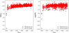Fig. 1. Derived infrared luminosity and star formation rate for all H-ATLAS sources and for the selected H-ATLAS sample. The H-ATLAS sample (red points) is relatively complete in infrared luminosity and SFR and was used as a basis for the SFG subsample.

Radio data are provided by the NRAO VLA Sky Survey (NVSS; Condon et al. 1998) and by the Faint Images of the Radio Sky at Twenty-cm (FIRST; Becker et al. 1994), both at 1.4 GHz. The NVSS covered 82% of the celestial sphere with a resolution of 45″ and a typical root mean square (RMS) noise of 0.45 mJy beam⁻¹. The FIRST survey covered over 10, 000 deg² (24% of the celestial sphere) at higher resolution (5.4″; Helfand et al. 2015) and a typical RMS of 0.15 mJy beam⁻¹.

A fraction of the radio luminosity in our sample might be of nuclear origin. To select SFGs as opposed to radio-loud active galactic nuclei (RL AGNs), we applied the Smolčić et al. (2017) 3σ radio excess criterion, according to which SFGs have L_1.4 GHz/SFR ratios below the redshift-dependent threshold,

$$\begin{array}{c}\hfill log\left(\frac{L_{1.4}}{\mathrm{SFR}}\right)=21.984\times {(1+z)}^{0.013},\end{array}$$(1)

with L_1.4 in W Hz⁻¹ and SFR in M_⊙ yr⁻¹. Sources below this threshold form the SFG subsample.

If a source is not detected by the NVSS or the FIRST survey, we computed the 5σ local RMS noise of the cutouts converted into radio luminosity (see Sect. 3) and applied the Smolčić et al. (2017) criterion. The SFG classification obtained in this way is conservative in the sense that it selects against AGN while possibly removing SFGs with a low SFR.

Our sample is not homogeneous in luminosity and redshift for the faintest sources, which, moreover, have unreliable distances. We therefore limited ourselves to z_spec > 0.001 and log(L_IR/L_⊙) > 7.5. Hereafter we refer to this subset as the H-ATLAS sample. This sample (red points in Fig. 1) contains 3328 sources. The SFG subsamples depend on the Smolčić et al. (2017) criterion and therefore depend on the radio map that was used to compute the radio luminosities. The SFG subsample based on FIRST radio luminosities contains 2368 sources, and the sample based on NVSS radio luminosities yields 553 sources.

To maximize the ratio of detections versus nondetections in stacks of radio maps, we defined extended subsamples for which we lowered the radio detection limit to 3σ in the stacking procedure described in Sect. 3.1. We label the results when the 3σ radio detection limit was used as the H-ATLAS 3σ sample and the corresponding SFG 3σ subsamples as the SFG 3σ samples. The SFG 3σ subsamples depend on the Smolčić et al. (2017) criterion and therefore depend on the radio map that was used to compute the radio luminosities. The SFG 3σ subsample based on the FIRST radio luminosities contains 2367 sources, and the sample based on NVSS radio luminosities contains 573 sources. The number of sources in different bins for each sample and subsample we defined above is given in Table 1.

3. Methods

We used median radio luminosity stacking to account for nondetections in the sample. In Sect. 3.1 we describe the stacking method and test for possible biases when NVSS and FIRST maps are used, while in Sect. 3.2 we describe the survival analysis method we used to estimate the impact of stacked images without detections.

3.1. Stacking procedure

Median stacking on the FIRST and NVSS maps was performed using cutouts centered on sources in each bin. These cutouts were then converted into 1.4 GHz radio luminosity density using the following equation:

$$\begin{array}{c}\hfill L_{1.4}=\frac{4\pi D_L^2}{{(1+z)}^{1-\alpha }}{S}_o,\end{array}$$(2)

where D_L is the luminosity distance, z is the spectroscopic redshift, S_o is the observed flux density, and α is the assumed spectral index, α = 0.7 (S_ν ∝ ν^−α).

To ensure proper positioning of cutouts, each of them was centered using a cubic convolution interpolation to the source position in the H-ATLAS catalog. After centering, stacked cutouts were produced by combining each pixel separately using median stacking. The 41  ×  41 px² stacked cutout and the 5σ noise estimate were used to infer the stacked radio luminosity densities using the source-extraction software BLOBCAT, which is designed to process radio-wavelength images (Hales et al. 2012). The RMS noise estimate that we used as input for BLOBCAT was computed excluding the central circular region (10 px radius) in the stacked cutout. The cutouts were limited in size to 41 px in each dimension in order to have a wide enough region in each cutout for RMS noise estimation without having to switch to the adjacent map for any source in the H-ATLAS sample.

The NVSS and FIRST maps have different resolutions. The 41 × 41 pix² area corresponds to 630″ × 630″ and 75″ × 75″, respectively. We considered an H-ATLAS source to have a valid radio counterpart if the position in the FIRST (NVSS) catalog was within a 10″ radius from the H-ATLAS position. The number of detected sources is shown for each bin in Table 1.

We tested whether radio luminosities derived using BLOBCAT may be affected by a systematic offset such as the snapshot bias (White et al. 2007). To this end, we compared them to luminosities derived from cataloged flux densities of detected sources. As shown in Fig. 2, we found that the offsets in both maps are within ±0.1 dex, and only the FIRST stacks show a significant (2σ) negative trend with radio luminosity. This trend, however, is not sufficiently large to explain the differences between the quantities derived in Sect. 4 when the FIRST and NVSS maps are used. We verified whether the inclusion of corrections might change the results of Sect. 4. Because no significant differences were found, no corrections were applied to the radio luminosity densities reported in this paper.

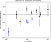Fig. 2. Logarithmic offsets between 1.4 GHz radio luminosities derived from stacked cutouts using BLOBCAT compared to the values derived from catalog flux densities. The black (blue) points refer to the subset of the H-ATLAS sample detected by the NVSS (FIRST) surveys.

3.2. Survival analysis

Stacking yielded 5σ detections for most but not all bins of the H-ATLAS and the SFG subsamples, as summarized in Table 1. A further complication is that various quantities of interest might have upper or lower limits in the two regression axes. An example of an upper limit is the L_1.4 nondetection, while an example of a lower limit is the q_IR nondetection due to the L_1.4 upper limit. For these cases, we extended the Sawicki (2012) method to the error-in-variable case by deriving its total least-squares variant. We estimated the flux upper limits as n times the RMS noise of the stacked cutout, with n = 5 for the 5σ BLOBCAT detection threshold and n = 3 for the 3σ threshold.

We modeled a dataset as a pair of values (x_i, y_i) drawn from normal distributions with variances ${\sigma }_{x,i}^2$ and ${\sigma }_{y,i}^2$. For upper limits, we assumed $x\le x_i^U$ or $y\le y_i^U$, and for lower limits, we assumed $x\ge x_i^L$ or $y\ge y_i^L$. For a general model f(x, θ), we adopted the likelihood function

$$\begin{array}{cc}& L(\theta )={\displaystyle \prod _{i\in D_x\cap D_y}\frac{1}{{\sigma }_{x,i}{\sigma }_{y,i}}\varphi \left(\frac{X_i-x_i}{{\sigma }_{x,i}}\right)\varphi \left(\frac{Y_i-f(\theta ,X_i)}{{\sigma }_{y,i}}\right)}\hfill \\ \hfill & \times {\displaystyle \prod _{i\in D_x\cap U_y}\frac{1}{{\sigma }_{x,i}{\sigma }_{y,i}}\varphi \left(\frac{X_i-x_i}{{\sigma }_{x,i}}\right)\mathrm{\Phi }\left(\frac{y_i^U-f(\theta ,X_i)}{{\sigma }_{y,i}}\right)}\hfill \\ \hfill & \times {\displaystyle \prod _{i\in D_x\cap L_y}\frac{1}{{\sigma }_{x,i}{\sigma }_{y,i}}\varphi \left(\frac{X_i-x_i}{{\sigma }_{x,i}}\right)(1-\mathrm{\Phi }\left(\frac{y_i^L-f(\theta ,X_i)}{{\sigma }_{y,i}}\right))}\hfill \\ \hfill & \times {\displaystyle \prod _{i\in U_x\cap D_y}\frac{1}{{\sigma }_{x,i}{\sigma }_{y,i}}\underset{-\infty }{\overset{x_i^U}{\int }}\mathrm{d}{X}_i\varphi \left(\frac{X_i-x_i}{{\sigma }_{x,i}}\right)\varphi \left(\frac{Y_i-f(\theta ,X_i)}{{\sigma }_{y,i}}\right)}\hfill \\ \hfill & \times {\displaystyle \prod _{i\in L_x\cap D_y}\frac{1}{{\sigma }_{x,i}{\sigma }_{y,i}}\underset{x_i^L}{\overset{\infty }{\int }}\mathrm{d}{X}_i\varphi \left(\frac{X_i-x_i}{{\sigma }_{x,i}}\right)\varphi \left(\frac{Y_i-f(\theta ,X_i)}{{\sigma }_{y,i}}\right)}\hfill \\ \hfill & \times {\displaystyle \prod _{i\in U_x\cap U_y}\frac{1}{{\sigma }_{x,i}{\sigma }_{y,i}}\underset{-\infty }{\overset{x_i^U}{\int }}\mathrm{d}{X}_i\underset{-\infty }{\overset{y_i^U}{\int }}\mathrm{d}{Y}_i\varphi \left(\frac{X_i-x_i}{{\sigma }_{x,i}}\right)\varphi \left(\frac{Y_i-f(\theta ,X_i)}{{\sigma }_{y,i}}\right)}\hfill \\ \hfill & \times {\displaystyle \prod _{i\in U_x\cap L_y}\frac{1}{{\sigma }_{x,i}{\sigma }_{y,i}}\underset{-\infty }{\overset{x_i^U}{\int }}\mathrm{d}{X}_i\underset{y_i^L}{\overset{\infty }{\int }}\mathrm{d}{Y}_i\varphi \left(\frac{X_i-x_i}{{\sigma }_{x,i}}\right)\varphi \left(\frac{Y_i-f(\theta ,X_i)}{{\sigma }_{y,i}}\right)}\hfill \\ \hfill & \times {\displaystyle \prod _{i\in L_x\cap U_y}\frac{1}{{\sigma }_{x,i}{\sigma }_{y,i}}\underset{x_i^L}{\overset{\infty }{\int }}\mathrm{d}{X}_i\underset{-\infty }{\overset{y_i^U}{\int }}\mathrm{d}{Y}_i\varphi \left(\frac{X_i-x_i}{{\sigma }_{x,i}}\right)\varphi \left(\frac{Y_i-f(\theta ,X_i)}{{\sigma }_{y,i}}\right)}\hfill \\ \hfill & \times {\displaystyle \prod _{i\in L_x\cap L_y}\frac{1}{{\sigma }_{x,i}{\sigma }_{y,i}}\underset{x_i^L}{\overset{\infty }{\int }}\mathrm{d}{X}_i\underset{y_i^L}{\overset{\infty }{\int }}\mathrm{d}{Y}_i\varphi \left(\frac{X_i-x_i}{{\sigma }_{x,i}}\right)\varphi \left(\frac{Y_i-f(\theta ,X_i)}{{\sigma }_{y,i}}\right),}\hfill \end{array}$$(3)

where D_X, U_X, and L_X (D_Y, U_Y and L_Y) mean detections and upper and lower limits in the x (y)-axis, respectively, while ϕ and Φ are the probability density and cumulative density functions for the normal distribution. We solved the integrals in Eq. (3) using the usual total least-squares approximation f(θ, X) = f(θ, x_i)+f′(x_i)(X_i − x_i). When there are N_x, U upper limits and N_x, L lower limits on the x-axis, we introduced the following variables:

$$\begin{array}{cc}& {\zeta }_i^U=\frac{x_i^U-x_i}{{\sigma }_{x,i}},i\in \{1,\cdots ,N_{x,U}\}\hfill \end{array}$$(4)

$$\begin{array}{cc}& {\zeta }_i^L=\frac{x_i-x_i^L}{{\sigma }_{x,i}},i\in \{1,\cdots ,N_{x,L}\},\hfill \end{array}$$(5)

which are nuisance parameters that need to be estimated in the same way as the parameters θ. The final expression is

$$\begin{array}{cc}& L(\theta ,{\zeta }_1^U,\cdots ,{\zeta }_{N_{x,U}}^U,{\zeta }_1^L,\cdots ,{\zeta }_{N_{x,L}}^L)\hfill \\ \hfill & ={\displaystyle \prod _{i\in D_y}\frac{1}{{\sigma }_i}\varphi \left(\frac{r_i}{{\sigma }_i}\right)\prod _{i\in D_x\cap U_y}\mathrm{\Phi }\left(\frac{r_i^U}{{\sigma }_i}\right)\prod _{i\in D_x\cap L_y}\mathrm{\Phi }\left(\frac{-r_i^L}{{\sigma }_i}\right)}\hfill \\ \hfill & \times {\displaystyle \prod _{i\in U_x\cap D_y}\mathrm{\Phi }({\zeta }_i^U\frac{{\sigma }_i}{{\sigma }_{x,i}}-r_i{f}_i^{\prime }\frac{{\sigma }_{x,i}}{{\sigma }_{y,i}{\sigma }_i})}\hfill \\ \hfill & \times {\displaystyle \prod _{i\in L_x\cap D_y}\mathrm{\Phi }({\zeta }_i^L\frac{{\sigma }_i}{{\sigma }_{x,i}}+r_i{f}_i^{\prime }\frac{{\sigma }_{x,i}}{{\sigma }_{y,i}})}\hfill \\ \hfill & \times {\displaystyle \prod _{i\in U_x\cap U_y}\underset{-\infty }{\overset{\frac{r_i^U}{{\sigma }_i}}{\int }}\mathrm{d}R\varphi \left(R\right)\mathrm{\Phi }({\zeta }_i^U\frac{{\sigma }_i}{{\sigma }_{x,i}}-R{f}_i^{\prime }\frac{{\sigma }_{x,i}}{{\sigma }_{y,i}})}\hfill \\ \hfill & \times {\displaystyle \prod _{i\in U_x\cap L_y}\underset{-\infty }{\overset{-\frac{r_i^L}{{\sigma }_i}}{\int }}\mathrm{d}R\varphi \left(R\right)\mathrm{\Phi }({\zeta }_i^U\frac{{\sigma }_i}{{\sigma }_{x,i}}+R{f}_i^{\prime }\frac{{\sigma }_{x,i}}{{\sigma }_{y,i}})}\hfill \\ \hfill & \times {\displaystyle \prod _{i\in L_x\cap U_y}\underset{-\infty }{\overset{\frac{r_i^U}{{\sigma }_i}}{\int }}\mathrm{d}R\varphi \left(R\right)\mathrm{\Phi }({\zeta }_i^L\frac{{\sigma }_i}{{\sigma }_{x,i}}+R{f}_i^{\prime }\frac{{\sigma }_{x,i}}{{\sigma }_{y,i}})}\hfill \\ \hfill & \times {\displaystyle \prod _{i\in L_x\cap L_y}\underset{-\infty }{\overset{-\frac{r_i^L}{{\sigma }_i}}{\int }}\mathrm{d}R\varphi \left(R\right)\mathrm{\Phi }({\zeta }_i^L\frac{{\sigma }_i}{{\sigma }_{x,i}}-R{f}_i^{\prime }\frac{{\sigma }_{x,i}}{{\sigma }_{y,i}})}\hfill \end{array}$$(6)

where we used the following abbreviations:

$$\begin{array}{cc}& {\widehat{x}}_i=\{\begin{array}{cc}{x}_i\hfill & \mathrm{detections}\hfill \\ x_i^U-{\sigma }_{x,i}{\zeta }_i^U\hfill & \mathrm{upper}\mathrm{limits}\hfill \\ x_i^L+{\sigma }_{x,i}{\zeta }_i^L\hfill & \mathrm{lower}\mathrm{limits}\hfill \end{array}\hfill \end{array}$$(7)

$$\begin{array}{cc}& f_i=f(\theta ,{\widehat{x}}_i)\hfill \end{array}$$(8)

$$\begin{array}{cc}& f_i^{\prime }=f^{\prime }(\theta ,{\widehat{x}}_i)\hfill \end{array}$$(9)

$$\begin{array}{cc}& r_i=y_i-f_i\hfill \end{array}$$(10)

$$\begin{array}{cc}& r_i^U=y_i^U-f_i\hfill \end{array}$$(11)

$$\begin{array}{cc}& r_i^L=y_i^L-f_i\hfill \end{array}$$(12)

$$\begin{array}{cc}& {\sigma }_i=\sqrt{{\sigma }_{y,i}^2+{(f_i^{\prime }{\sigma }_{x,i})}^2}.\hfill \end{array}$$(13)

We maximized the likelihood in Eq. (6) using the Markov chain Monte Carlo (MCMC) method implemented in the package emcee (Foreman-Mackey et al. 2013). We started by giving uniform priors for θ and ζs. Because ζs are just normalized x values that are expected to be mostly positive by definition, we used a fixed range ζ_i ∈ ⟨ − 1, 10].

We tested the survival analysis codes using Monte Carlo simulations to fit the linear model. We made 5000 simulations for samples of sizes in the range from 5 to 15 data points, chosen to encompass the number of bins in the real dataset. We chose to simulate linear models with both slopes and intercepts in the intervals [ − 2, 2]. The simulated y-values were centered on the chosen linear model, with deviations drawn from the normal distribution 𝒩(0, σ²), where σ was chosen to vary in the range [10⁻⁴, 10⁻¹]. The error on σ_x was set equal to σ. Furthermore, the probability of detection, p_D, was chosen to be between 0.4 and 1. The probability that a point is an upper limit in each axis was chosen from a uniform distribution in the interval [0, 1 − p_D], and the probability for a data point to be a lower limit on an axis was computed so that the probabilities summed to one. The labels of a detection, upper and lower limit were then drawn for each data point and for each axis from these distributions. If a point was an upper limit in the x(y) axis, its value was shifted upwards by 5σ_x (5σ_y). Conversely, if it was a lower limit in the x(y) axis, its value was shifted downwards by 5σ_x (5σ_y).

The differences between the slopes and intercepts obtained from simulations and the input values are shown in Fig. 3 as functions of the ratio of the number of lower and upper limits on both axes (R_x, L, R_x, U, R_y, L, R_x, L), of log σ and of the size of the sample. No systematic offsets were found in these distributions. We also quantified this finding by computing the P-value in each bin of R_x, L, R_x, U, R_y, L, R_x, L, log σ, and size. To compute the P-values, we first computed the standard Z-scores (i.e., the difference between the input and simulated value divided by the standard deviation of the simulations) of the differences between simulated, a, and input slopes, $\widehat{a}$, as well as those between simulated, b, and input intercepts, $\widehat{b}$. Standard deviations were computed from the MCMC-derived covariance matrix. The P-values of each estimate in each bin were then combined using the Fisher method (see, e.g., Fisher 1925). The resulting P-values, shown in Fig. 4, suggest that there is no significant offset in any bin below log σ ∼ −1.5 at a significance value of 5%, which is comparable to the log σ-s in the (sub)sample (ranging from −1.6 to −1.2). By considering the derived parameter differences and Z-scores, we conclude that there is an expected bias in the derived parameters, but that the bias is lower than the parameter errors and therefore is not large enough to be relevant for our analysis.

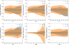Fig. 3. Differences between the Monte Carlo simulated linear model parameters and the corresponding simulation inputs. The results are shown for bins in the ratio of the number of upper and lower limits on the x- and y-axes (Rx, L, Rx, U, Ry, L, and Ry, U) as well as for bins of the dispersion σ and of the size of the sample (see Sect. 3.2 for details). The blue lines show the median differences between the simulated, a, and input slopes, $\widehat{a}$, and the orange lines show the same difference for the simulated intercept, b, and its input in the simulation, $\widehat{b}$. The shaded intervals are the intervals between the 16th and 84th percentile in each bin.

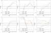Fig. 4. P-values for the differences between the Monte Carlo simulated linear model parameters and their corresponding simulation inputs. The blue lines show the P-values computed using the Z-scores of the differences between the simulated, a, and input slopes, $\widehat{a}$, and the orange lines show the P-values computed for the simulated intercept. The bins are the same as in Fig. 3 (see Sect. 3.2 for details). The dashed, dot-dashed, and dotted black lines show the 10%, 5%, and 1% confidence limits, respectively, as reference.

4. Results

We stacked the NVSS and FIRST map cutouts using L_IR and SFR bins, as detailed in Table 1. We separately considered the H-ATLAS sample, the SFG subsample, the H-ATLAS 3σ sample, and the SFG 3σ subsample.

The IR luminosity-SFR relation is shown in Fig. 5, and the radio luminosity densities for the different IR luminosity and SFR bins are shown in Fig. 6. For each bin, the radio luminosity density was derived using BLOBCAT on the stacked cutout image. If no signal was detected, a 5σ (3σ for the extended sample) limit was computed from the RMS noise in the stacked cutout.

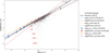Fig. 5. Relation between SFR and LIR for various (sub) samples, with their respective error bars. The various samples are identified in the legend by the binning strategy (LIR and SFR bins) and by the respective sample type (H-ATLAS and SFG). Solid lines represent the best-fitting relations for each sample, listed in Table 2, and correspond in color to the data points. The black dots represent SFR and LIR for individual sources in the H-ATLAS sample.

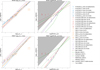Fig. 6. Radio luminosity density log L1.4 derived for bins of IR luminosity (left panels) and SFR (right panels), with their error bars and best-fitting lines listed in Table 2. Upper limits are shown as arrows corresponding in color to detections (points). The top row refers to NVSS cutouts, and the bottom row shows FIRST cutouts. Non-SFG samples, i.e., samples not cleaned using the Smolčić et al. (2017) criterion (excluded region shown as a shaded interval), show a strong radio luminosity excess at a given SFR due to the presence of RL AGNs.

The results of the stacking procedure and of survival analysis can be found in Table 2. In this table we show the results of our fits. When there were no upper or lower limits on either axis, an orthogonal distance regression model fit was used for the linear model, while survival analysis was used when limits were present on either axis. The results are plotted in Fig. 7 for a subset of fits for which the relative errors of the two linear-model parameters were lower than 20%.

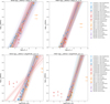Fig. 7. Best-fitting lines from Table 2 for which the relative errors on the two parameters a and b are lower than 20%. Solid lines represent the best-fitting relations for each sample, listed in Table 2, while their corresponding confidence intervals are shown by the shaded bands. The left panels show results for the NVSS cutouts, and the right panels show the results for the FIRST cutouts. Detections are marked with points, and arrows are used to show nondetections, both with accompanying error bars on both axes.

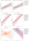Fig. 7. continued.

We tested linear relation fits connecting logSFR and the logarithm of the IR luminosity, log L_IR. We tested for the significance of nonlinearities in the log L_IR − logSFR relation by fitting a linear relation to the transformed value, log L_IR − logSFR as a function of IR luminosity, which tests for the presence of a quadratic (log L_IR) term in the log L_IR − logSFR dataset. We applied the same fitting strategy to the radio luminosity, exploring its dependence on SFR and IR luminosity, and tested for possible nonlinearities by fitting a linear relation to the transformed value, log L_1.4 − logSFR, as a function of log L_1.4. We additionally verified whether the q_IR parameter depends on IR and radio luminosity, or if it can affect the log L_1.4 − logSFR value.

5. Discussion

We chose to compare our results with a selection of local studies and studies with a wide redshift range at or converted to 1.4 GHz. This is representative of the published relations (see Sect. 1). Yun et al. (2001) observed an IRAS galaxy sample cross-matched to the NVSS survey in a similar redshift range as our study, while Bell (2003) assembled a diverse sample of galaxies with accompanying far ultraviolet, optical, IR, and radio luminosities to explore the infrared-radio correlation. Murphy et al. (2011) analyzed Ka-band observations of star-forming regions in NGC 6946, which they expanded to a sample of 56 nearby galaxies at 33 GHz with a median beam width of 25 arcsec in Murphy et al. (2012). Delhaize et al. (2017) studied the q parameter out to z ∼ 5 using a survival analysis technique to account for IR and 3 GHz radio nondetections, while Bonato et al. (2017) studied the radio luminosity function of SFGs and searched for nonlinearity in the relation of radio luminosity to SFR out to z ∼ 5. Gurkan et al. (2018) studied the relation between LOFAR and H-ATLAS observations of SFGs, while Matthews et al. (2021) studied a large, local, volume-limited sample of SFGs selected at 1.4 GHz.

Figure 5 (L_IR versus SFR) shows consistency with the Murphy et al. (2012) linear relation between L_IR and SFR for both SFG samples with regard to the slope, which they derived using the 33 GHz data and a Kroupa (2001) initial mass function. We also fit the log L_IR/SFR ratio versus L_IR with a linear model. We find a small positive slope at a significance of 5σ for all samples and binning strategies, except for the SFR bins using the H-ATLAS sample, for which the error on the slope was too large for us to accurately determine the slope. Overall, using SFR bins yielded a smaller slope (∼0.1), while the L_IR binning produced a slope of ∼0.2. In both cases, however, the data indicate higher L_IR/SFR ratios for higher IR luminosity, generally corresponding to higher obscuration by dust. This suggests that the MAGPHYS fits may either slightly overestimate L_IR or underestimate the SFR for the more obscured galaxies.

In Fig. 6 we show the correlations between the radio luminosity density, L_1.4, derived from the NVSS and FIRST maps, and L_IR or SFR. The NVSS radio luminosities, indicated by the best-fitting lines in the left panels of Fig. 6, are substantially higher than the FIRST radio luminosities, which is consistent with extended emission of our low-z galaxies being missed at the FIRST resolution, as pointed out by Jarvis et al. (2010). Therefore we focused on NVSS luminosities. Our results for the SFG samples are consistent with the linear relation between L_1.4 and L_IR by Bell (2003). The relations by Yun et al. (2001) and by Delhaize et al. (2017) are somewhat higher and somewhat lower than our mean relation, respectively. Our results do not support the sublinear relation between L_1.4 and L_IR reported by Gurkan et al. (2018), nor the substantially superlinear relation by Matthews et al. (2021).

As expected, H-ATLAS sample data points, which also contain RL AGNs, show substantial deviations from a linear relation at low-IR luminosities. The fitted slope of the log L_1.4 − log L_IR relation based on NVSS data is sublinear at the 7σ level. A similar trend, with an even more significant sublinearity, is seen in the log L_1.4 − logSFR relation for NVSS flux densities and SFR bins. On the other hand, in the other cases, the log L_1.4 − log L_IR relation is superlinear. In all cases, the quality of the fit is quite poor. This complex situation arises because of the contaminating effect of RL AGNs, whose radio emission dominates especially at low and high SFRs or L_IRs, flattening or steepening the relations, respectively. Moreover, local radio AGNs are generally hosted by passive early-type galaxies whose IR luminosity may be mostly due to dust heated by old stellar populations rather than to star formation.

We find that the upper limits do not significantly affect the trends when they are accounted for using survival analysis. The simulations suggest that the datasets with a higher percentage of upper limits should be progressively less reliable, but large systematic offsets in the derived linear model parameters are not expected. The log L_1.4/SFR ratio fits do not point toward a statistically significant nonlinearity, even when the upper limits are accounted for. We therefore conclude that the survival analysis results are consistent with the linear L_1.4–SFR relation by Murphy et al. (2011). There is no evidence of a stronger decline of the L_1.4/SFR ratio at low luminosity that was obtained based on one of the relations derived by Bonato et al. (2017) from the comparison of the local SFR function with the local 1.4 GHz luminosity function.

The q_IR does not show any statistically significant dependence on radio luminosity. The dependence on L_IR in the case of the H-ATLAS samples is the trivial consequence of the fact that the radio luminosity of RL AGNs is independent of the SFR, which enters the definition of q_IR and is correlated to L_IR. The L_1.4/SFR ratio shows no statistically significant correlation with q_IR. We find no statistically significant differences between the results for the H-ATLAS and H-ATLAS–3σ samples and for the SFG and SFG–3σ samples.

The radio-excess criterion is not perfect in discerning AGNs from SFGs. Smolčić et al. (2017) defined the moderate-to-high radiative luminosity AGN (HLAGN) by a combination of X-ray, MIR color–color, and SED-fitting criteria. The low-to-moderate radiative luminosity AGN (MLAGN) are defined by either a color selection criterion combined with the absence of Herschel detections (quiescent MLAGN) or by the 3σ radio excess. Because we use a Herschel–selected sample, we do not expect contamination by radio-quiet MLAGN, and the radio-excess criterion eliminates the presence of radio-excess MLAGN. The contamination by HLAGN is harder to remove because only about 30% of HLAGN exhibit radio excess. In Fig. 6 we show the region that was excluded in the definition of the SFG subsamples as a shaded interval. We find that the only H-ATLAS sample bins that are significantly affected by this cut are those with a lower SFR. Delhaize et al. (2017) found that the HLAGN have a lower q_IR value than SFGs, which could in part explain the large dispersion in the fitting parameters for our q_IR fits.

6. Summary and conclusions

We have investigated the IR-radio and SFR-radio correlations for a sample that is complete to over 91% of 3328 z  ≤  0.1 galaxies (H-ATLAS sample). All galaxies have spectroscopic redshifts. The sample was drawn from the H-ATLAS catalog, which covers three equatorial fields that encompass a total area of 161.6 deg². The wealth of multifrequency data that is available for these sources has allowed us to determine total IR (8–1000 μm) luminosities and SFR for all sources using the MAGPHYS package (da Cunha et al. 2008).

Radio data were provided by the FIRST and NVSS surveys. We extracted 1.4 GHz flux densities from radio images and checked for possible biases. The FIRST flux densities are systematically lower than those of the NVSS, as expected because the FIRST 5 arcsec beam misses a substantial fraction of extended emission at the low redshifts of our sources. We therefore focused on NVSS flux densities.

An SFG subsample was built by removing from the H-ATLAS sample all sources showing a radio excess according to the Smolčić et al. (2017) criterion. However, only a minor fraction of sources are above the 5σ detection threshold: 81 FIRST (104 NVSS) SFG detections out of a total of 84 FIRST (138 NVSS) detections. Sources below the threshold were binned in log(L_IR), and for each bin, we performed a stacking analysis on the NVSS and FIRST images. Statistical 5σ detections were obtained for most bins, 7 (10) out of 18 FIRST (NVSS) log L_IR bins and 10 (10) out of 13 FIRST (NVSS) logSFR bins. For bins lacking detection, we extended the Sawicki (2012) survival analysis technique.

Our sample has allowed us to investigate the L_IR–SFR, the L_1.4–L_IR and the L_1.4–SFR correlations. In all cases, the H-ATLAS sample showed much larger dispersions than the SFG sample, betraying the presence of a substantial contamination by radio AGNs. This contamination is stronger at the highest and at the lowest radio luminosities and tends to yield superlinear or sublinear L_1.4 versus L_IR and L_1.4 versus SFR relations, respectively. To better test low luminosities and low SFRs, we also considered 3σ detections. The results from the 5σ and 3σ samples are fully consistent with each other. The SFG samples have allowed us to probe the ranges 7.5 ≲ log(L_IR/L_⊙)≲13, −3.5 ≲ log(SFR/M_⊙ yr⁻¹)≲2.5 and 20 ≲ log(L_1.4/W Hz⁻¹) ≲ 22. In these low-luminosity or low-SFR ranges, deviations from linearity are expected to show up more clearly.

Our results are fully consistent with the linear relations between L_IR and SFR by Murphy et al. (2012), between L_1.4 and L_IR by Bell (2003), and between L_1.4 and SFR by Murphy et al. (2011). However, our data are also consistent with the small deviations from linearity that were reported by some studies. The normalization of our L_1.4 versus L_IR relation is intermediate between those by Yun et al. (2001), which is somewhat higher, and by Delhaize et al. (2017), which is somewhat lower.

Acknowledgments

This work is financed within the Tenure Track Pilot Program of the Croatian Science Foundation and the École Polytechnique Fédérale de Lausanne and the Project TTP-2018-07-1171 Mining the Variable Sky, with funds of the Croatian-Swiss Research Program. Amirnezam Amiri thanks Habib Khosroshahi (IPM), Ali Dariush (Cambridge University), and Mohammad H. Zhoolideh Haghighi (IPM) for useful discussions. Krešimir Tisanić thanks Mladen Novak (Max-Planck-Institut für Astronomie).

References

All Tables

All Figures

	Fig. 1. Derived infrared luminosity and star formation rate for all H-ATLAS sources and for the selected H-ATLAS sample. The H-ATLAS sample (red points) is relatively complete in infrared luminosity and SFR and was used as a basis for the SFG subsample.
In the text

	Fig. 2. Logarithmic offsets between 1.4 GHz radio luminosities derived from stacked cutouts using BLOBCAT compared to the values derived from catalog flux densities. The black (blue) points refer to the subset of the H-ATLAS sample detected by the NVSS (FIRST) surveys.
In the text

Fig. 3. Differences between the Monte Carlo simulated linear model parameters and the corresponding simulation inputs. The results are shown for bins in the ratio of the number of upper and lower limits on the x- and y-axes (Rx, L, Rx, U, Ry, L, and Ry, U) as well as for bins of the dispersion σ and of the size of the sample (see Sect. 3.2 for details). The blue lines show the median differences between the simulated, a, and input slopes, $\widehat{a}$, and the orange lines show the same difference for the simulated intercept, b, and its input in the simulation, $\widehat{b}$. The shaded intervals are the intervals between the 16th and 84th percentile in each bin.

In the text

Fig. 4. P-values for the differences between the Monte Carlo simulated linear model parameters and their corresponding simulation inputs. The blue lines show the P-values computed using the Z-scores of the differences between the simulated, a, and input slopes, $\widehat{a}$, and the orange lines show the P-values computed for the simulated intercept. The bins are the same as in Fig. 3 (see Sect. 3.2 for details). The dashed, dot-dashed, and dotted black lines show the 10%, 5%, and 1% confidence limits, respectively, as reference.

In the text

Fig. 5. Relation between SFR and LIR for various (sub) samples, with their respective error bars. The various samples are identified in the legend by the binning strategy (LIR and SFR bins) and by the respective sample type (H-ATLAS and SFG). Solid lines represent the best-fitting relations for each sample, listed in Table 2, and correspond in color to the data points. The black dots represent SFR and LIR for individual sources in the H-ATLAS sample.

In the text

Fig. 6. Radio luminosity density log L1.4 derived for bins of IR luminosity (left panels) and SFR (right panels), with their error bars and best-fitting lines listed in Table 2. Upper limits are shown as arrows corresponding in color to detections (points). The top row refers to NVSS cutouts, and the bottom row shows FIRST cutouts. Non-SFG samples, i.e., samples not cleaned using the Smolčić et al. (2017) criterion (excluded region shown as a shaded interval), show a strong radio luminosity excess at a given SFR due to the presence of RL AGNs.

In the text

Fig. 7. Best-fitting lines from Table 2 for which the relative errors on the two parameters a and b are lower than 20%. Solid lines represent the best-fitting relations for each sample, listed in Table 2, while their corresponding confidence intervals are shown by the shaded bands. The left panels show results for the NVSS cutouts, and the right panels show the results for the FIRST cutouts. Detections are marked with points, and arrows are used to show nondetections, both with accompanying error bars on both axes.

In the text

	Fig. 7. continued.
In the text

References

- Abazajian, K. N., Adelman-McCarthy, J. K., Agüeros, M. A., et al. 2009, ApJS, 182, 543 [Google Scholar]
- Aversa, R., Lapi, A., de Zotti, G., Shankar, F., & Danese, L. 2015, ApJ, 810, 74 [NASA ADS] [CrossRef] [Google Scholar]
- Becker, R. H., White, R. L., & Helfand, D. J. 1994, Astronomical Data Analysis Software and Systems III, 61, 165 [NASA ADS] [Google Scholar]
- Bell, E. F. 2003, ApJ, 586, 794 [Google Scholar]
- Berta, S., Lutz, D., Santini, P., et al. 2013, A&A, 551, A100 [NASA ADS] [CrossRef] [EDP Sciences] [Google Scholar]
- Bonato, M., Negrello, M., Mancuso, C., et al. 2017, MNRAS, 469, 1912 [Google Scholar]
- Bourne, N., Dunne, L., Maddox, S. J., et al. 2016, MNRAS, 462, 1714 [NASA ADS] [CrossRef] [Google Scholar]
- Calistro Rivera, G., Williams, W. L., Hardcastle, M. J., et al. 2017, MNRAS, 469, 3468 [Google Scholar]
- Chabrier, G. 2003, PASP, 115, 763 [Google Scholar]
- Chi, X., & Wolfendale, A. W. 1990, MNRAS, 245, 101 [Google Scholar]
- Clemens, M. S., Scaife, A., Vega, O., & Bressan, A. 2010, MNRAS, 405, 887 [NASA ADS] [Google Scholar]
- Colless, M., Dalton, G., Maddox, S., et al. 2001, MNRAS, 328, 1039 [Google Scholar]
- Condon, J. J. 1992, ARA&A, 30, 575 [Google Scholar]
- Condon, J. J., Cotton, W. D., Greisen, E. W., et al. 1998, AJ, 115, 1693 [Google Scholar]
- da Cunha, E., Charlot, S., & Elbaz, D. 2008, MNRAS, 388, 1595 [Google Scholar]
- de Jong, T., Klein, U., Wielebinski, R., et al. 1985, A&A, 147, L6 [Google Scholar]
- de Jong, J. T. A., Kuijken, K., Applegate, D., et al. 2013, Messenger, 154, 44 [Google Scholar]
- Delhaize, J., Smolčić, V., Delvecchio, I., et al. 2017, A&A, 602, A4 [NASA ADS] [CrossRef] [EDP Sciences] [Google Scholar]
- Devereux, N. A., & Eales, S. A. 1989, ApJ, 340, 708 [NASA ADS] [CrossRef] [Google Scholar]
- Driver, S. P., Norberg, P., Baldry, I. K., et al. 2009, Astron. Geophys., 50, 5.12 [NASA ADS] [CrossRef] [Google Scholar]
- Eales, S., Dunne, L., Clements, D., et al. 2010, PASP, 122, 499 [NASA ADS] [CrossRef] [Google Scholar]
- Edge, A., Sutherland, W., Kuijken, K., et al. 2013, Messenger, 154, 32 [Google Scholar]
- Fisher, R. 1925, Statistical Methods For Research Workers (Edinburgh: Oliver and Boyd) [Google Scholar]
- Foreman-Mackey, D., Hogg, D. W., Lang, D., & Goodman, J. 2013, PASP, 125, 306 [Google Scholar]
- Gavazzi, G., Cocito, A., & Vettolani, G. 1986, ApJ, 305, L15 [CrossRef] [Google Scholar]
- Gurkan, G., Hardcastle, M. J., Smith, D. J. B., et al. 2018, MNRAS [Google Scholar]
- Hales, C. A., Murphy, T., Curran, J. R., et al. 2012, MNRAS, 425, 979 [Google Scholar]
- Helfand, D. J., White, R. L., & Becker, R. H. 2015, ApJ, 801, 26 [NASA ADS] [CrossRef] [Google Scholar]
- Helou, G., Soifer, B. T., & Rowan-Robinson, M. 1985, ApJ, 298, L7 [Google Scholar]
- Jarvis, M. J., Smith, D. J. B., Bonfield, D. G., et al. 2010, MNRAS, 409, 92 [Google Scholar]
- Kennicutt, R. C., & Evans, N. J. 2012, ARA&A, 50, 531 [NASA ADS] [CrossRef] [Google Scholar]
- Klein, U., Wielebinski, R., & Thuan, T. X. 1984, A&A, 141, 241 [NASA ADS] [Google Scholar]
- Kroupa, P. 2001, MNRAS, 322, 231 [NASA ADS] [CrossRef] [Google Scholar]
- Lawrence, A., Warren, S. J., Almaini, O., et al. 2007, MNRAS, 379, 1599 [Google Scholar]
- Liske, J., Baldry, I. K., Driver, S. P., et al. 2015, MNRAS, 452, 2087 [Google Scholar]
- Magnelli, B., Ivison, R. J., Lutz, D., et al. 2015, A&A, 573, A45 [NASA ADS] [CrossRef] [EDP Sciences] [Google Scholar]
- Mancuso, C., Lapi, A., Cai, Z.-Y., et al. 2015, ApJ, 810, 72 [Google Scholar]
- Martin, D. C., Fanson, J., Schiminovich, D., et al. 2005, ApJ, 619, L1 [Google Scholar]
- Massardi, M., Bonaldi, A., Negrello, M., et al. 2010, MNRAS, 404, 532 [NASA ADS] [Google Scholar]
- Matthews, A. M., Condon, J. J., Cotton, W. D., & Mauch, T. 2021, ApJ, 914, 126 [CrossRef] [Google Scholar]
- Mauch, T., & Sadler, E. M. 2007, MNRAS, 375, 931 [Google Scholar]
- Murphy, E. J., Condon, J. J., Schinnerer, E., et al. 2011, ApJ, 737 [Google Scholar]
- Murphy, E. J., Bremseth, J., Mason, B. S., et al. 2012, ApJ, 761 [Google Scholar]
- Pilbratt, G. L., Riedinger, J. R., Passvogel, T., et al. 2010, A&A, 518, L1 [NASA ADS] [CrossRef] [EDP Sciences] [Google Scholar]
- Planck Collaboration VI, 2020, A&A, 641, A6 [NASA ADS] [CrossRef] [EDP Sciences] [Google Scholar]
- Prandoni, I., & Seymour, N. 2015, Advancing Astrophysics with the Square Kilometre Array (AASKA14), 67 [Google Scholar]
- Price, R., & Duric, N. 1992, ApJ, 401, 81 [NASA ADS] [CrossRef] [Google Scholar]
- Sargent, M. T., Schinnerer, E., Murphy, E., et al. 2010, ApJS, 186, 341 [Google Scholar]
- Sawicki, M. 2012, PASP, 124, 1208 [NASA ADS] [CrossRef] [Google Scholar]
- Smolčić, V., Delvecchio, I., Zamorani, G., et al. 2017, A&A, 602, A2 [NASA ADS] [CrossRef] [EDP Sciences] [Google Scholar]
- Valiante, E., Smith, M. W., Eales, S., et al. 2016, MNRAS, 462, 3146 [NASA ADS] [CrossRef] [Google Scholar]
- Voelk, H. J. 1989, A&A, 218, 67 [NASA ADS] [Google Scholar]
- Wang, L., Gao, F., Duncan, K. J., et al. 2019, A&A, 631, A109 [NASA ADS] [CrossRef] [EDP Sciences] [Google Scholar]
- White, R. L., Helfand, D. J., Becker, R. H., Glikman, E., & de Vries, W. 2007, ApJ, 654, 99 [Google Scholar]
- Wright, E. L., Eisenhardt, P. R. M., Mainzer, A. K., et al. 2010, AJ, 140, 1868 [Google Scholar]
- Yun, M. S., Reddy, N. A., & Condon, J. J. 2001, ApJ, 554, 803 [Google Scholar]
All Tables
Derived fits for the stacked sources in the NVSS and FIRST maps of the H-ATLAS and SFG samples.