| Issue |
A&A
Volume 657, January 2022
|
|
|---|---|---|
| Article Number | A40 | |
| Number of page(s) | 15 | |
| Section | Planets and planetary systems | |
| DOI | https://doi.org/10.1051/0004-6361/202141865 | |
| Published online | 24 December 2021 | |
VLT spectropolarimetry of comet 67P: dust environment around the end of its intense southern summer
1
Institut für Geophysik und Extraterrestrische Physik, Technische Universität Braunschweig,
Mendelssohnstr. 3,
38106
Braunschweig,
Germany
e-mail: y.kwon@tu-braunschweig.de
2
Armagh Observatory, College Hill,
Armagh
BT61 9DG,
Northern Ireland,
UK
3
Max Planck Institute for Solar System Research,
Justus-von-Liebig-Weg 3,
37077
Göttingen,
Germany
4
Department of Astronomy, University of Maryland,
College Park,
MD
20742,
USA
5
LATMOS, Sorbonne Université, CNRS, UVSQ, Campus Pierre et Marie Curie,
4 place Jussieu,
75005
Paris,
France
6
Institute for Astronomy, University of Edinburgh, Royal Observatory,
Edinburgh
EH9 3HJ,
UK
7
INAF – Osservatorio Astrofisico di Arcetri,
50125
Firenze,
Italy
Received:
23
July
2021
Accepted:
1
October
2021
Context. A cornucopia of Rosetta and ground-based observational data sheds light on the evolution of the characteristics of dust particles from comet 67P/Churyumov-Gerasimenko (hereafter 67P) with seasons, implying the different dust environments in the source regions on the surface of the comet.
Aims. We aim to constrain the properties of the dust particles of 67P and therefrom diagnose the dust environment of its coma and near-surface layer at around the end of the southern summer of the comet.
Methods. We performed spectropolarimetric observations for 67P dust over 4000–9000 Å using the ESO/Very Large Telescope from January–March 2016 (phase angle ranging from ~26° –5°). We examined the optical behaviours of the dust, which, together with Rosetta colour data, were used to search for dust evolution with cometocentric distance. Modelling was also conducted to identify the dust attributes compatible with the results.
Results. The spectral dependence of the polarisation degree of 67P dust is flatter than that found in other dynamical groups of comets in similar observing geometry. The depth of its negative polarisation branch appears to be a bit shallower than in long-period comets and might be getting shallower as 67P repeats its apparitions. Its dust colour shows a change in slope around 5500 Å, (17.3 ± 1.4) and (10.9 ± 0.6)% (1000 Å)-1, shortward and longward of the wavelength, respectively, which are slightly redder but broadly consistent with the average of Jupiter-family comets.
Conclusions. Observations of 67P dust in this study can be attributed to dust agglomerates of ~100 μm in size detected by Rosetta in early 2016. A porosity of 60% shows the best match with our polarimetric results, yielding a dust density of ~770 kg m-3. The compilation of Rosetta and our data indicates the dust’s reddening with increasing nucleus distance, which may be driven by water-ice sublimation as the dust moves out of the nucleus. We estimate the possible volume fraction of water ice in the initially ejected dust as ~6% (i.e. the refractory-to-ice volume ratio of ~14).
Key words: comets: general / comets: individual: 67P/Churyumov-Gerasimenko / methods: observational / methods: numerical / techniques: polarimetric / techniques: spectroscopic
© ESO 2021
1 Introduction
The two-year rendezvous with comet 67P/Churyumov-Gerasimenko (hereafter 67P) by the ESA/Rosetta spacecraft from 3.60 au inbound on 2014 August 6 to 3.83 au outbound on 2016 September 30 provides an unprecedented database of cometary dust. In particular, the onboard Micro-Imaging Dust Analysis System (MIDAS) unravels a hierarchical nature of the cometary dust: ≳100-micrometre dust agglomerates consist of approximately tens of micrometre dust aggregates, which are in turn comprised of solid sub-micrometre dust grains (monomers) of a similar size as interstellar dust, highlighting the importance of dust evolution indigenous to our planetary system (Bentley et al. 2016; Mannel et al. 2016, 2019). The aggregates or agglomerates can be classified by the mechanical strength pertinent to their porosity (Fulle et al. 2016; Güttler et al. 2019). The prevailing group of dust particles in the coma varies in the porosity (the volume of voids in a particle) with the comet’s season (Longobardo et al. 2020), indicating that the source regions activated in different orbital positions have different properties. Observations showing such seasonal effects thus emphasise the importance of constraining the properties of the ejected dust particles as diagnostics for the dust environment across the nucleus surface (Marschall et al. 2020 and references therein).
The coordinated ground-based campaign of 67P had supplemented the Rosetta observations throughout the mission phase by monitoring large-scale (≳103 km in cometocentric distance) comet activity in various observing modes, such as photometry, spectroscopy, and polarimetry, at different spectral domains (see Table 1 in Snodgrass et al. 2017 for the summary). The campaign is aimed at better understanding and ultimately forging a comprehensive reference of cometary activity and dust constituents by linking in situ and ground-based observations. As a consequence, the following three aspects of 67P were identified in common by the observations. Firstly, strong seasonal effects of the comet induce discernible asymmetry in macroscopic dust coma morphology and gas production rates between the pre- and post-perihelion phases, while the overall activity peaked at ≲1 month in its outbound orbit (Boehnhardt et al. 2016; Snodgrass et al. 2016; Hadamcik et al. 2016; Opitom et al. 2017; Ivanova et al. 2017; Knight et al. 2017). Secondly, changes in the radial profile and polarisation degree of 67P dust on either side of the perihelion indicate that its pre-perihelion dust coma characteristics could be attributed to the presence of large-sized (millimetre-to-centimetre) particles, whereas particles dominating the coma around and just after perihelion would be smaller and/or fluffier dust (Hadamcik et al. 2016; Rosenbush et al. 2017). Thirdly, all the above-mentioned traits seem to have remained constant over the last three apparitions (Hadamcik et al. 2016; Opitom et al. 2017; Knight et al. 2017).
Despite the cogent evidence in the evolution of the global activity pattern of 67P and its dust particles throughout the perihelion passage, the characteristics of the dust, particularly its porosity, are still open to be discussed. A constraint on the dust porosity helps to better understand the mechanisms on the comet surface that shape the surface morphology (Longobardo et al. 2020; Marschall et al. 2020) and macroscopic coma activity (Kwon et al. 2019). However, limitations in the observing geometry of the Rosetta spacecraft that confined it to mostly terminator orbits around the comet, together with a limitation in the sensitivity of the onboard dust analysers, put little constraints on the property of interest (Thomas et al. 2019). For ground-based observations, the fast brightness decrease of 67P on its way outwards from perihelion and a coarse spatial resolution of the telescopes used (typically larger than a few thousand kilometres) made it challenging to obtain high signal-to-noise ratio (S/N) inner coma data (Knight et al. 2017). A study on the nature of the cometary dust under such circumstances thus necessitates adopting bigger diameter telescopes with an efficient observing strategy for the dust study.
At this juncture, polarimetry provides a valuable additional dimension of interpretation on the light scattered by cometary dust (Bohren & Huffman 1983). Polarisation as an intensity ratio reflects the properties of the scattering dust particles, differing from the intensity in widely used photometry or spectroscopy that is mainly sensitive to the number density of the dust particles within an aperture or a slit of a certain width, which alone tends to provide a degenerate solution on the dust properties. Imaging polarimetry observations of the dust of various comets at different phase angles showcase the usefulness of polarimetry well, showing distinct dust coma structures characterised by different types of dust particles on the polarisation map, which were invisible on the intensity map (Renard et al. 1996; Hadamcik & Levasseur-Regourd 2003a). Spectropolarimetry further provides polarimetric and spectroscopic information simultaneously, thus allowing us to obtain information on the polarisation degree, the position angle of polarisation, their variations about wavelength, and dust colour, free of gas contamination (e.g. Fig. 2 in Kwon et al. 2018). Few studies have been made in this observing mode because of the small number of available facilities and small limiting magnitudes (Kiselev et al. 2015).
Here, we present new spectropolarimetric observations of comet 67P from the European Southern Observatory’s Very Large Telescope (VLT). The VLT’s 8-m diameter and dual-beam polarimetry optics allowed us to conduct spectropolarimetric observations of 67P’s faint coma (V -band apparent magnitude of ~16.34 mag1) around the end of its southern summer, with negligible atmospheric effects. We performed observations at three epochs in about a monthly cadence in early 2016. Combining the results of the Rosetta dust studies with the modelling of our observations, we estimated the porosity of the dust particles of 67P and discuss the possible amount of embedded water ice and the refractory-to-ice ratio of the dust. Section 2 describes the observational methods and data analyses, and in Sect. 3, we present the results, which are discussed in Sect. 4. Finally, in Sect. 5, we present a summary.
Observational geometry and instrument settings.
2 Observations and data analysis
In this section, we describe the observational circumstances and data analyses. The journal of our observational geometry and instrument settings is summarised in Table 1.
2.1 Observations
A three-epoch optical spectropolarimetric observation of comet 67P was conducted from UT 2016 January 12 to March 04 in approximately monthly cadence using a polarimeter attached to the 8.0-m diameter VLT at the Paranal Observatory (70°24′10′′.1W, 24°37′31′′.5S, 2635 m) in Chile. FORS2 is a multi-purpose optical instrument mounted on the Cassegrain focus of the UT1 telescope at VLT. A dual-beam polarimeter2, consisting of a rotatable half-wave plate (HWP) and a Wollaston prism (WP), is located upstream of two 2k × 4k CCD detectors with the plate scale of 0′′.125 pixel-1 (with the pixel size of 15 × 15 μm2) and the fieldof view (FoV) of 6′.8 × 6′.8. In spectropolarimetry (PMOS) observing mode with the standard resolution (SR) collimator, we used the 2 × 2 binning for fainter targets such as 67P around this term of observations, yielding the pixel scale of 0′′.25 pixel-1.
The rotatable HWP introduces a phase-shift between the components of the electric field parallel andperpendicular to its optic axis and rotates them at fixed positions separated by 22°.5. The HWP is followed by a WP which splits the light into two orthogonally polarised (extraordinary and ordinary) beams, separated by 22′′ (a Wollaston Mask is introduced before the HWP to avoid overlapping of the two beams; Fig. 2.7 in FORS2 user manual). The last optical element before the detector is a grism, which may be preceded by an order-separating filter. The instrument design allows the user to implement a beam-swapping technique, in which two beams carrying light polarised in opposite directions are swapped during an observing series in which the HW is oriented at 0°, 22°.5, 45°, and 67°.5, etc., with respect to the principal plane of the WP. This allows one to largely suppress the effects of instrumental polarisation (e.g. Bagnulo et al. 2009). For our observations, we used grism 300V with no order-separating filter, covering the spectral range 3800 Å–9300 Å. We used a 1′′.75 slit for a spectral resolution of ~250. The same instrument setup was adopted for all three observing epochs, with exposure times of 280 s for the January observation and 300 s for the February and March observations per single exposure, achieving the total exposure time of 2240 and 2400 s, respectively. Median seeing was 0′′.66, 0′′.58, and 0′′.99 for the January, February, and March observations, respectively.
2.2 Data analysis
In all epochs, we obtained two sets of exposures (N = 2 in Table 1), that is, a total of eight fits files of 16 light elements at the eight different HWP position angles from 0° to 157°.5 in 22°.5 intervals. A beam-swapping technique implemented took the first set at the HWP angle of 0°, 22°.5, 45°, and 67°.5, and the second set, which was rotated 90° from the first one, at the HWP angle of 90°, 112°.5, 135°, and 157°.5 in a row. Cosmicrays were removed using the L.A. Cosmic tool (van Dokkum 2001). Lamp calibration spectra (He+1, HgCd+2, Ar+1, and Ar+2) for wavelength calibration were taken under the identical observational configurations (Grism_300V) after the target observations in 2 × 2 binning mode. We did not conduct flux calibration because we took ratios of the light elements to derive the Stokes parameters. Wavelength-calibrated spectra of each light component were then extracted using APALL in IRAF. In APALL, thebackground of each spectrum was fitted by a linear function and then the spectrum was traced by the third-order Chebyshev function. The resultant one-dimensional spectrum showed the root-mean-square (RMS) of ~0.07– 0.35 (pixel)-1. We repeated these extraction steps using six different aperture sizes (corresponding to 1000–7500 km in cometocentric distance).
The small RMS in the pre-processing stage confirmed that the subtraction of the slowly varying background feature works well, while the small FoV of the slit (22′′ in width) limits the elimination of bright telluric lines, particularly ~5500, 6300, 6870, and 7600 Å for O2 from the observed data. The remnants of the subtraction are discernible in the final spectrum, showing slight deviations with larger error bars than the ambient points. We discarded the edge of the wavelength regions (λ < 4000 Å and λ > 9000 Å) that showed large fluctuations and binned the extracted data points to have a wavelength interval of ~52 Å. We found radial variations in neither count nor shape of the spectra obtained with different aperture sizes. For instance, Figs. A.1–A.3 show negligible differences between the spectra with the aperture sizes of 1000 and 7500 km; furthermore, spectra with other aperture sizes also showed no difference within the uncertainties. This is probably because the diffuse background coma structures visible in the sky images of Fig. 1 were too feeble to be observed with the exposure time applied in the PMOS mode, mainly allowing us to sample the central part of the coma of 67P. Since the larger the aperture, the more significant error becomes, we decided to analyse the spectrum extracted with the aperture size corresponding to 1000 km in cometocentric distance.
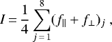
Stokes parameters of the total intensity I and the linear polarisation degree Q and U were derived using the difference method (Bagnulo et al. 2009). The reduced Stokes parameters q and u were calculated as
![\begin{equation*}q\,{=}\,\frac{Q}{I}\,{=}\,\frac{1}{2N} \sum_{i\,{=}\,1}^{N} \bigg[\bigg(\frac{f_{||} - f_{\perp}}{f_{||} + f_{\perp}} \bigg)_{X} - \bigg(\frac{f_{||} - f_{\perp}}{f_{||} + f_{\perp}} \bigg)_{X + 45^{\circ}} \bigg]~,\end{equation*}](/articles/aa/full_html/2022/01/aa41865-21/aa41865-21-eq1.png) (1)
(1)
![\begin{equation*}u\,{=}\,\frac{U}{I}\,{=}\,\frac{1}{2N} \sum_{i\,{=}\,1}^{N} \bigg[\bigg(\frac{f_{||} - f_{\perp}}{f_{||} + f_{\perp}} \bigg)_{Y} - \bigg(\frac{f_{||} - f_{\perp}}{f_{||} + f_{\perp}} \bigg)_{Y + 45^{\circ}} \bigg]~,\end{equation*}](/articles/aa/full_html/2022/01/aa41865-21/aa41865-21-eq2.png)
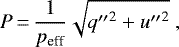
where N is the number of the pair of exposures (N = 2 in this study); f|| and f⊥ denote the photon counts of ordinary and extraordinary rays at each HWP position angle β; β = X ∈ 0° and 90° for q estimation, while β = Y ∈ 22°.5 and 112°.5 for u estimation; and Stokes I, the total intensity, can be expressed as
 (3)
(3)
where j is the eight HWP position angles of 0°, 22°.5, ..., 157°.5 in π/8 intervals. Since we did not carry out absolute flux calibration in this study, the multiplicative factor (1/4) in Eq. (3) is of little importance. The usage of ratios between extraordinary and ordinary ray fluxes (split by the WP) in Eq. (1) allowed us to remove instrumental effects such as flat fielding and the change in sky transparency between exposures (Bagnulo et al. 2009).
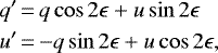
The derived reduced Stokes parameters were then corrected for the wavelength-dependent deviation of the HWP position angle from the nominal angle (i.e. chromatism; Bagnulo et al. 2009) using the equations of
 (4)
(4)
where ϵ is the deviation angle tabulated in the FORS2 user manual and the webpage3. Next, we corrected for the wavelength-dependent instrumental polarisations qinst and uinst using Eq. (7) in Cikota et al. (2017) and converted the Stokes parameters in the instrument reference system to the celestial reference system as follows:
 (5)
(5)
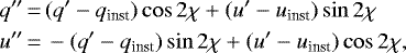
where χ denotes the WP position angle, counted counterclockwise from north to eastward, which corresponds to the header keyword of ADA.POSANG. The fraction of linear polarisation (i.e. the polarisation) and its position angle are then expressed as
 (6)
(6)
where peff is the polarisation efficiency at each wavelength. Since the peff was measured at discrete wavelengths of 4150–10 575 Å, we interpolated the trend line of the peff to obtain the value at our wavelength positions.
In solar system science, the polarisation is usually expressed in a reference system whose reference direction is perpendicular to the scattering plane (a plane containing the Sun–comet–Earth). We thus transformed P and θP (measured with respect to the equatorial system) into the reference system using
 (8)
(8)
where ϕ represents the position angle of the scattering plane, the sign of which (± in Eq. (9)) was chosen to satisfy 0 ≤ (ϕ ± π/2) ≤ π (Chernova et al. 1993). We note that θr can be used to check the reliability of the data as follows. In a random distribution of the coma dust, θr ~90° (~0°) is expected when the polarisation vector aligns perpendicular (parallel) to the scattering plane, and the resultant Pr becomes positive (negative). Uncertainties, including photon noise on P (Eq. (3) in Bagnulo et al. 2017) and the conversion to Pr, were estimated by following standard error propagation methods. In our datasets, points free from the remnant of major telluric lines (~5500, 6300, 6870, and 7600 Å for O2) enabled us to retrieve reliable Pr values, showing the appropriate θr alignments as expected.
3 Results
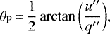
Figure 1 shows sky images of 67P at three epochs obtained from a single exposure. The coma structure is highly asymmetric, showing south-eastern and sunward jets with feeble dust tails both in the anti-solar (−r⊙) and negative velocity (−v) directions. The neck-line structure was visible at all epochs, but most clearly in March. It stretches up to ~2.9 × 10⁵ km in the sky plane beyond the figure, as confirmed by previous ground-based observations (Snodgrass et al. 2017; Rosenbush et al. 2017; Knight et al. 2017). In this section, we present the dependences of 67P’s Pr (Eq. (8)) on the wavelength (Sect. 3.1) and phase angle (Sect. 3.2), and the dependence of the intensity (Eq. (3)) on the wavelength (i.e. colour; Sect. 3.3).
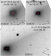 |
Fig. 1 Sky images of 67P obtained from a single exposure. The phase angle and equivalent filter range are provided on top of each figure. Panel awas obtained with a 120-s exposure, while panels b and cwere obtained with a 60-s exposure. Panels a and b cover the FoV of 1′.0 × 1′.0, while panel cspans 2′.0 × 1′.2 to encompass the neck-line structure. North is up and east is to the left. The level of brightness was inverted and arbitrarily adjusted to enhance weak coma structures. The 1000-km-sized aperture applied in this study is overlaid as a magenta box, covering the inner coma part. The solid and dashed arrows denote the Sun–comet radius vectors and the comet’s negative heliocentric velocity vectors, respectively. Background structures are either stars or cosmic rays. |
3.1 Dependence of the polarisation degree on the wavelength
Figures 2–4 show the wavelength dependence of the polarisation degree, Pr (λ), of 67P dust onUT 2016 January 12, February 04, and March 04, respectively. The weighted mean and error of the θr points over 4000–9000 Å are also provided in panel b of each figure to check the reliability of data processing. In January (Fig. 2), the dust’s polarisation position angle is aligned to the perpendicular direction to the scattering plane (θr ~ 0°), such that the resultant Pr has a positive sign, while Pr of 67P dust in February and March (Figs. 3 and 4) has a negative sign because of the polarisation vector along the scattering plane (θr ~ 90°). Except for several deviating points with large error bars due to the remnants of the sky emission lines (Sect. 2.2), we do not find any gas emission line features at all epochs. This is consistent with the absence of a spherical gas coma structure in the sky images (Fig. 1) and also with the results of the spectroscopic study using the VLT/FORS2 with the longer exposure time (300–600 s) taken on UT 2016 March 04 (Opitom et al. 2017). Although Opitom et al. (2020) later find the weak water-sublimation-driven [OI] emission at 6300 Å around the nucleus in 2016 March in VLT’s integral field unit spectrograph (MUSE) data, this line is overlapped with the sky emission line, thus difficult for our data to discriminate the two lines.
In order to quantify the spectral dependence of Pr, we performed a linear least-square fitting. Since the comet’s faintness makes the data points at both ends of the covered wavelength range fluctuate, we used only the intermediate points in the 4550–7560 Å region for fitting and applied the solution to the whole wavelength range (4000–9000 Å). The concept of ‘Polarimetric colour (PC)’ is defined as
 (10)
(10)
where Pr (λ1) and Pr (λ2) are the Pr values in percent measured at the wavelengths of λ1 = 4550 Å and λ2 = 7560 Å, respectively.Conventionally, a positive PC is labelled as red, and a negative PC is labelled as blue. With the linear equations of a ⋅ λ+ b, where a and b are the slope and y intercept of the fitting function, we obtain the PC: (0.14 ± 0.08)% (1000 Å)-1 for Fig. 2; (−0.03 ± 0.07)% (1000 Å)-1 for Fig. 3; and (0.03 ± 0.12)% (1000 Å)-1 for Fig. 4. Provided that we exclude the deviating data points on the short-end wavelength from consideration (particularly severe in March at λ < 5000 Å due to the low brightness of the comet), the PC values on either side of 5500 Å (the wavelength around which the dust colour changes its slope; Sect. 3.3) are consistent within the error ranges with those obtained from a total wavelength coverage.
Next, we compare 67P’s spectral dependence of Pr with those ofother comets taken at a similar range of α. The PC of the cometary dust depends on α. In general, for most comets, the PC is red over the wavelength of interest at α > 25°, around which the PC is relatively neutral but quickly increases the slope as α increases. The PC at α < 20° tends to be slightly blue (Kolokolova et al. 2004; Kiselev et al. 2015). Figure 5 shows the Pr distribution of cometary dust on the wavelength at the α range of 0° –35° adopted from the NASA/PDS comet polarimetric archive (Kiselev et al. 2017) and from Bagnulo et al. (2021). We selected data only taken with the narrow-band continuum filters and at multi-wavelength (quasi-)simultaneously (i.e. at least on the same day) to minimise the possible gas contamination and systematic difference induced by the nucleus rotation. Since the UC narrow-band filter (3656/84 Å) somewhat suffers from C3 emission (Kiselev & Velichko 1996), we focus on the wavelength dependence in the range of >4000 Å.
In Fig. 5, we can see a change of sign of PC around the vertical dashed line from negative at α ≲ 22° (the negative polarisation branch; NPB) to positive at larger α (the positive polarisation branch; PPB), as expected (Kiselev et al. 2015). Both in pre- and post-perihelion phases, the comets, regardless of their dynamical groups, tend to follow this general trend. On the other hand, 67P dust shows a much flatterPC both in the NPB and PPB than other comets, particularly compared to non- and long-period comets.
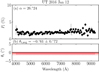 |
Fig. 2 Pr of 67P dust in % (a) and the mean and 1σ error of the position angle of Pr with regard to the scattering plane (θr) as a functionof the wavelength (b) observed at α = 26°.4 on UT 2016 January 12. The black points in panel a were binned to have wavelength intervals of ~52 Å. The large error bars result from the remnants of the skylines that were not perfectly subtracted due to the limited slitwidth. The red solid and upper and lower dashed lines inpanel b indicate the weighted mean of θr (θr, avg) and its error(the standard deviation divided by the square of the number of the data points), respectively. The black line marks θr = 0°, the expected value when the dust is distributed randomly in the coma. |
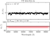 |
Fig. 3 Same as Fig. 2, but at α = 18°.47 on UT 2016 February 04. The black line indicates θr = 90°, the expected value when the dust is distributed randomly in the coma. |
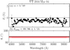 |
Fig. 4 Same as Fig. 2, but at α = 5°.49 on UT 2016 March 04. The black line indicates θr = 90°, the expected value when the dust is distributed randomly in the coma. |
3.2 Dependence of the polarisation degree on phase angle
Low albedos and aggregate structures of cometary dust lead to a general α dependence of Pr, parameterised by a shallow NPB with an average minimum polarisation Pmin ≈ −1.5% at αmin ≈ 10°, and an inversion angle where Pr changes its sign from negative to positive at α0 ≈ 22°, and a bell-shaped PPB with a maximum polarisation Pmax ≈ 25–30% at αmax ~ 95° in the wavelength region that interests us (Kiselev et al. 2015). The most probable explanation for the change of Pr ’s sign is that the interference effects between the multiple-scattered light around the back-scattering region yields the change in the alignment of the polarisation vector parallel to the scattering plane (Muinonen et al. 2015).
We first compiled all Pr of 67P dust from the NASA/PDS comet polarimetric archive (Kiselev et al. 2017) to compare the phase angle dependence with our data. Given that the majority of the archival data were taken in the red domain (central wavelength of 6200–7300 Å) and that the highest S/N in our data was achieved in the 5000–7000 Å range with a flat wavelength dependence (Figs. 2–4), we decided to utilise the archival data taken in the red domain. We thus took the weighted mean of our data points over 5000–7000 Å at each epoch and used the result as a nominal value. Only narrow-band Pr and the data proven to be free from gas contamination in the red domain were selected from the archive for the analysis. The archival data having either very small or large apertures were excluded. To minimise possible dependence of Pr on the aperture size, we adopted the data points having the aperture size in the same order of magnitude as ours (1000 km in radius), resulting in the range of 1000–10 000 km cometocentric distance (on average of ~2300 km). The dataset with the 10 000-km-sized aperture comes from Stinson et al. (2016), where the comet was in its outbound orbit, showing weak but stable coma activity. The large scatter of their data across the fitted line seems to introduce no bias (black circles in Fig. 6), such that we decided to use them. The average Pr dependence on the phase angle, Pr(α), of the selected data was then obtained using the empirical trigonometric function of Lumme & Muinonen (1993):
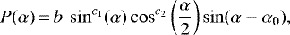 (11)
(11)
where b, c1, c2, and α0 are the wavelength-dependent free parameters shaping the curve.
Figure 6 shows the resultant Pr(α) of 67P dust. The number of pre-perihelion data (open symbols) of 67P is insufficient to fit the trend, and thus the trends for the data as a whole (solid curve) and those in post-perihelion data (dashed curve) are examined. The best-fit parameters of the curve for all 67P data are b = 52.32 ± 20.87%, c1 = 1.01 ± 0.24, c2 = 9.99 ± 5.82, and α0 = 21°.71 ± 0°.51. Those for 67P post-perihelion data are b = 68.10 ± 40.10%, c1 = 1.21 ± 0.32, c2 = 9.99 ± 10.32, and α0 = 22°.07 ± 0°.57. Since the number of 67P data is small and they cover α < 40°, the uncertainty of the fitting parameter b, which is related to the amplitude of the curves(i.e. the maximum Pr at α ~ 95°), becomes significant. The result shows that the pre-perihelion data points appear to be located in the lower side of the average trend both in the NPB and PPB. Hadamcik et al. (2016) attribute such a systematic Pr (α) difference of 67P dust between the pre- and post-perihelion to the different characteristics of the dust. Although the small number of pre-perihelion data prevents us from making an in-depth analysis, we confirm the consistently lower position of the pre-perihelion data with regard to the fitted curves, supporting the evolution of the dust properties throughout the perihelion passage.
We also investigate how the Pr(α) varies with time. We subtracted the fitted Pr at the given α from the observed (ΔPr = Pr, obs − Pr, fitted) and took the weighted mean of the ΔPr in the same apparition. Since it is better to analyse the data in the NPB separately from those in the PPB (Muinonen et al. 2015), we delimited the α range of <22° to focus on the NPB. Figure 7 shows the departure of the Pr of 67P dust (ΔPr) in different apparitions from the general trend of the phase curve (i.e. the solid line in Fig. 6 now equals ΔPr = 0). The ΔPr and its error are (−0.30 ± 0.10), (0.25 ± 0.13), and (0.46 ± 0.15)% for the 1983, 2009, and 2015 apparitions, respectively. We did not include the pre-perihelion point (open orange circle) for the retrieval. Although the Pr(α) difference between the last two apparitions is statistically insignificant, we find an overall decrease in the absolute Pr values in the NPB (i.e. a decrease in the depth of the NPB) as the apparition proceeds.
Finally, we compare the Pr(α) of dust between 67P and other comets. The narrow-band data (or broad-band ones unambiguously proved to be free from gas contamination) taken in the red domain from the NASA/PDS archive (Kiselev et al. 2017) and the data of an extrasolar comet, 2I/Borisov, taken in RF filter (6550/1650 Å; Bagnulo et al. 2021) are used for this comparative study. Again, the average trend was estimated from Eq. (11) for the data whose aperture size ranges from ~1000 to 10 000 km (on average ~4000 km in cometocentric distance). We excluded unique comets C/1995 O1 (Hale-Bopp) and 2I/Borisov from the fitting due to their significant Pr excess compared to the majority of comets (Hadamcik & Levasseur-Regourd 2003b; Kikuchi 2006; Bagnulo et al. 2021) and the large aperture size (for Hale-Bopp). Figure 8 shows the results of the compilation. The LPC and NPC stand for long- and non-period comets, respectively, in which the comets used are C/1990 K1 (Levy), C/1996 B2 (Hyakutake), C/2000 WM1 (LINEAR), C/2001 A2 (LINEAR), C/2009 P1 (Garradd), and C/2010 R1 (LINEAR). The JFC and ETC stand for Jupiter-family and Encke-type comets, respectively, and the used comets are 17P/Holmes, 67P, 74P/Smirnova-Chernykh, 78P/Gehrels, 152P/Helin-Lawrence, and 290P/Jager. The points of 67P were used for fitting, but they are shown separately (as red diamonds) for comparison with other comets. The comet shows a similar Pr distribution with other JFC and ETC within the measurement uncertainties.
Most comets show deviations from the average to both directions, being on the upper and lower parts of the fitted curve. Such a dispersion ispartially a result of an unstable state in the cometary activity, but it would also be the consequence of observations made by various teams in slightly different wavelength domains (e.g. Lasue et al. 2009). However, C/1995 O1 (Hale-Bopp) around its perihelion (25° < α < 35°) always shows excessively high Pr values compared to the majorityof comets. The Pr of 2I/Borisov shows a typical value in the NPB, but as high as those of Hale-Bopp in the PPB (Bagnulo et al. 2021). For other comets, we did not find such a significant difference. In the NPB, the short-period comets (i.e. JFC and ETC) tend to extend to slightly smaller absolute Pr values than LPC and NPC. The Oort-cloud origin comets tend to spread towards more negative Pr values.
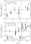 |
Fig. 5 Polarimetric colour (PC) of comets over the α range of 0° –35°. All data points except 67P in this study are quoted from the NASA/PDS comet polarimetric archive (Kiselev et al. 2017) and from Bagnulo et al. (2021). Panels a and b present the data in pre-perihelion (180° < ν < 350°, where ν means the true anomaly) and post-perihelion (10° < ν ≤ 180°), respectively. There are no available points around the perihelion (350° ≤ ν ≤ 10°). Red circles of 67P are obtained from the least-square linear fit of 67P dust (Figs. 2–4), and their error bars indicate 1σ uncertainties of the fitting. Black open symbols were derived from the comet data observed by aperture polarimetric observations. Thus, the error bars of their PCs were derived from the error propagation of Pr values measured at discrete wavelength points. ‘Garradd’ and ‘LINEAR’ denote comets C/2009 P1 (Garradd) and C/2000 WM1 (LINEAR), respectively. |
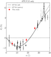 |
Fig. 6 Polarisation of 67P dust versus phase angle. Open and filled symbols denote the pre- and post-perihelion data, respectively. Black symbols are the archival data (Kiselev et al. 2017) where different shapes indicate the datasets obtained by different works: circle (Myers & Nordsiseck 1984), square (Hadamcik et al. 2016), triangle (Hadamcik et al. 2010), polygon (Stinson et al. 2016), and diamond (Rosenbush et al. 2017). Red diamonds denote our spectropolarimetric data. Background grey symbols (Kiselev et al. 2017) are excluded from the analysis due to the significant difference in the aperture sizes from ours. The solid and dashed curves indicate the average dependence derived from Eq. (11) for the data as a whole and in post-perihelion, respectively. The best-fit parameters of the curves are provided in the text. |
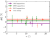 |
Fig. 7 Departure of the Pr of 67P dust in each apparition from to the average trend. The black fitting line in Fig. 6 now corresponds to the horizontal dashed lines at ΔPr = 0. The horizontal solid lines and shaded areas denote the weighted mean and error, in which the colour scheme follows the symbols in the legend. Open and filled symbols denote the pre- and post-perihelion data of 67P dust. Only post-perihelion data were used to estimate ΔPr. |
 |
Fig. 8 Polarisation of all available comets’ dust versus phase angle. The black solid line and shaded areas denote the average trend of the dependence and its 3σ error, respectively. As in Fig. 6, open and filled symbols denote the pre- and post-perihelion data, while background grey circles represent data points discarded from the fitting because of either their large aperture size (≫10 000 km in cometocentric distance) and/or the possible gas contamination. All symbols are the archival data of Kiselev et al. (2017), except for the four points of 2I/Borisov (Bagnulo et al. 2021) and three points of 67P (this study). We exclude unique comets C/1995 O1 (Hale-Bopp) and 2I/Borisov from the fitting, since their Pr has been found to be significantly higher. The red diamonds edged with black lines are our spectropolarimetric data. The best fit parameters of the fitted curve are b = 25.69 ± 1.27%, c1 = 0.67 ± 0.02, c2 = (1.54 ± 0.85) × 10-13, and α0 = 21°.25 ± 0°.14. A detailed description of the legend is provided in the text. |
3.3 Dust colour
In addition to the PC, we can also obtain the wavelength dependence of the intensity (i.e. dust colour) by dividing the Stokes I of the dust (Eq. (3)) by that of the solar spectrum. To this end, we observed a solar analogue HD 67010 (Datson et al. 2015) under the identical optics to the target observations (PMOS mode), with the HWP angle of 0° on UT 2016 February 16. Extraction and binning of the stellar spectrum were performed in the same way as described in Sect. 2, yielding the extraction RMS of ~0.02–0.13 (pixels)-1. Assuming that the star is unpolarised, we obtained its intensity by adding the counts of f|| and f⊥ and multiplying the sum by 2. A difference in airmass between the solar analogue (on average 2.59) and 67P observations (Table 1) can be compensated for by using
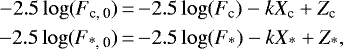 (12)
(12)
where the subscripts c and * indicate a quantity for the comet and the star. We note that Fc, 0 and F*, 0 are the fluxes of 67P dust and the solar analogue’s outside atmosphere, respectively, and Fc and F* are the counterparts measured at the airmass Xc (I in Eq. (3)) and X* (2.59). The k denotes the wavelength-dependent extinction coefficient. Assuming that the zero points on the observing nights of 67P (Zc) and the star (Z*) are roughly the same, Eq. (12) reduces to
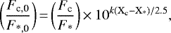 (13)
(13)
the left side of which is the dust colour. For the k values, we refer to the Paranal coefficients published by Patat et al. (2011). The zero points measured inthe B, V, and R filters at the four observing epochs are in fact slightly different within ~0.01 mag. This introduces an uncertainty of ≲3% in comparing the relative brightness measured on different nights.
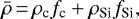
Figure 9a shows the resultant relative brightness distribution of 67P dust over 4000–8000 Å. Although an incomplete correction of telluric absorption lines, particularly O2 and H2 O lines, leaves bumpy structures longwards of ~6500 Å at all epochs, the dust continuum colour compensated for the atmospheric effects remains nearly the same over the two months. A change in the slope of the colour (i.e. the inflection point) appears around 5500 Å, which is consistent with the previous studies (Frattin et al. 2017; Filacchione et al. 2020; Opitom et al. 2020). To compare the colour presented here with other comets, we derived the normalised reflectivity S′ in the unit of % (1000 Å)-1 using
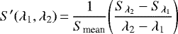 (14)
(14)
(Jewitt & Meech 1986), where λ1 and λ2 are the short-end and long-end wavelengths considered. We set λ1 = 4000 Å and λ2 = 5500 Å shortwards of the inflection point (‘blue’ side), and λ1 = 5600 Å and λ2 = 7900 Å longwards of the inflection point (‘red’ side). We note that  ,
,  , and Smean denote the relative brightness at λ1 and λ2 and the mean relative brightness in the wavelength range considered, respectively. Three colours in Fig. 9a were combined into the average, yielding (17.3 ± 1.4)% (1000 Å)-1 for the blue side and (10.9 ± 0.6)% (1000 Å)-1 for the red side.
The S′ of 67P dust in Fig. 9b is in line with the results of previous studies (Storrs et al. 1992; Schleicher 2006; Hadamcik & Levasseur-Regourd 2009; Snodgrass et al. 2016; Rosenbush et al. 2017 that show a slightly larger (i.e. redder colour) yet still broadly consistent S′ of 67P dust with the typical colour range of short-period comets. Grün et al. (2016) report a three-hour-long outburst event accompanied by factors >100 increase of the near-nucleus coma brightness when Rosetta was at an altitude of 34 km on UT 2016 February 19. However, any significant aftermath of the event seems invisible in our colour data. Compared to variations of the brightness and the Afρ parameter (a proxy of the dust mass-loss rate of a comet; A’Hearn 1984) from photometry showing a slight increase after the outburst on UT 2016 February 19 (Boehnhardt et al. 2016; Grün et al. 2016), the stable colour trend shown in our data would indicate that the dust properties over the two months remain more or less constant.
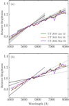 |
Fig. 9 Relative brightness of 67P dust normalised at 5500 Å. (a) The dust colour slopes (Eq. (14)) are shown as the solid lines with 3σ fitting errors in grey regions. (b) Two solid black lines indicate the lower (5 ± 2% (1000 Å)-1) and upper (18 ± 2% (1000 Å)-1) reflectivity limits of the dust of nine comets over 3500–6500 Å, respectively (Jewitt & Meech 1986). The thick grey solid and dashed lines indicate the average reflectivity trend and standard deviation of 31 active comets (8.4 ± 3.6% (1000 Å)-1) over 3540–9050 Å used in Solontoi et al. (2012). |
4 Discussion
In this section, we describe the dust environment of 67P based on the results in Sect. 3, in conjunction with the observationsobtained from in situ and previous ground-based studies. We first constrained the size and structure of 67P dust during this period (Sect. 4.1) and the possible amount of embedded water ice and the refractory-to-ice ratio of the dust particles (Sect. 4.2).
4.1 Constraints on the properties of 67P dust
This study covers two months on the brink of the second equinox of 67P (at rH = 2.63 au on UT 2016 March 21). The sub-solar latitude of the nucleus during the time of our observations varied from about −13° to −1° (Preusker et al. 2017), in which the comet’s dust activity had already passed its peak and decreased smoothly (Knight et al. 2017). In the following, we suggest the most plausible properties of the dust attributable to our results in Sect. 3 by considering three main aspects – the composition, size, and porosity of the dust.
4.1.1 Conjecture based on the observational evidence in this study
The primary constituents of cometary dust are silicates (mainly in the form of olivine and pyroxene), carbonaceous materials (amorphous carbon and organics), Fe-bearing sulfides, and ice (Levasseur-Regourd et al. 2018). Our colour data showing the broad consistency with active short-period comets (Fig. 9b) would not indicate much of a difference in 67P dust from the typical dust in compositional terms of view. However, its slightly redder colour than the average would allow us to rule out the predominance of materials whose transparency decreases with wavelengths (e.g. water ice) in the dust particles (Kolokolova & Jockers 1997). The polarimetric phase curve of 67P dust in the red domain, which is consistent with the trend of most comets but shows a slightly shallower depth of the NPB than those of non- and long-period comets (Fig. 8) and 67P in previous apparitions (Fig. 7), support the ordinary composition of 67P dust dominated by absorbing materials (Petrova et al. 2001; Hadamcik & Levasseur-Regourd 2009). A large imaginary part of the complex refractive index (i.e. high absorptivity) can also explain the neutral PC of 67P dust (Fig. 5) that is flatter than those of other comets in similar observing geometry (Kolokolova & Jockers 1997).
In terms of the dust’s physical attributes, the dominance of large4 over small dust5 can explain such a red colour (Kolokolova et al. 1997), small PC values (Gustafson & Kolokolova 1999), and shallower NPB depth (Hadamcik & Levasseur-Regourd 2009) of 67P dust. All the results are also compatible with a low level of dust porosity. Laboratory experiments and computer modelling of cometary dust have shown that as the packing density of the cometary dust increases, the depth of the NPB becomes shallower (Petrova et al. 2001; Hadamcik & Levasseur-Regourd 2009; Kolokolova et al. 2015), the dust colour reddens (Gustafson & Kolokolova 1999), and the PC becomes less red (Gustafson & Kolokolova 1999).
Taken as a whole, observations of 67P dust obtained with the 1000 km-sized aperture in this study could be ascribed to the dominance of coarse (larger than tens of micrometres in size), rather compact dust particles in the coma, whose light scattering characteristics are similar to those of the evolved near-surface dust layer likely common for short-period comets (e.g. Hadamcik & Levasseur-Regourd 2009; Biele et al. 2015; Spohn et al. 2015; Kwon et al. 2018). The Comet Nucleus Sounding Experiment by Radiowave Transmission (CONSERT), onboard Rosetta and its Philae lander, indeed provides evidence of a shallow subsurface of about 20 m in depth, which is less porous and thus denser than the interior of the nucleus (Kofman et al. 2020).
4.1.2 Comparison with the Rosetta observations and estimation of the plausible dust porosity
In early 2016, mainly two different types of dust particles would coexist in the sampled 1000-km-sized coma: (i) particles directly ejected from the nucleus and (ii) particles which were ejected and had either fallen back to the nucleus surface, followed by re-ejection around perihelion, or remained in bound orbits without fallback (Agarwal et al. 2016; Longobardo et al. 2020). Type (ii) dust particles are primarily decimetre-sized aggregates (Mottola et al. 2015; Agarwal et al. 2016; Pajola et al. 2017), and their large size and compactness make them less sensitive to the gas drag and solar radiation pressure than fluffier dust counterparts (Gundlach et al. 2020; Fulle et al. 2020). They tend to linger in the circumnuclear coma of 67P (<100 km; e.g. Bertini et al. 2019), and we expect that their contribution to the scattering cross-section in the 1000 km aperture would be small. For type (i) dust particles, Rosetta observations classify them into two families – compact and fluffy dust aggregates. Although the definition of the classification is slightly different between the Grain Impact Analyser and Dust Accumulator (GIADA) (Della Corte et al. 2015) and the Cometary Secondary Ion Mass Analyzer (COSIMA) (Hornung et al. 2016; Langevin et al. 2016), they both show that fluffy dust particles have a fractal dimension of <2 and are prone to be fragmented, while compact counterparts have a porosity below 90% with higher tensile strengths and density (Levasseur-Regourd et al. 2018). The former prevails in the dust coma around perihelion, but contributes less beyond the outbound distance of ~2 au (Longobardo et al. 2020). Relatively compact dust aggregates would then become the dominant signal in the background coma at the epochs we covered, showing no significant fragmentation as they move out of the nucleus at least in the <500 km distance range (Frattin et al. 2021 and references therein).
In a synthesis paper of 67P dust, Güttler et al. (2019) classify dust particles collected throughout the mission depending on the size, porosity, and strength, and they confirm the dominance of the role of ‘porous dust agglomerates’ in the observed light scattering phenomena. This type of dust has a typical size of ~100 μm with the porosity ranging from 10 to 95% (Güttler et al. 2019 and references therein). A majority of compact dust aggregates, which are initially named by COSIMA and GIADA, belong to this dominant group based on their physical properties. Therefore, we use the terminology of ‘porous dust agglomerates’ in the following, instead of compact dust aggregates, to demonstrate the dust with a lower porosity than fluffy dust aggregates. The composition of 67P dust in such a size scale shows similarity to a large extent with other cometary dust probed by past space missions, in which Mg-rich silicates and carbonaceous materials account for the majority of refractory components (Levasseur-Regourd et al. 2018).
In order to understand how porosity influences the polarimetric behaviour of such dust particles, we numerically simulated the light scattering of the dust with a representative size of 100 μm in radius and the following three different cases of the dust porosity: 60, 80, and 95%. The first porosity value considered represents the solid-like (non-fragmenting) dust (Hornung et al. 2016), the second one is for the dust with an intermediate porosity, and the last one is for the fluffiest particle in the ‘porous dust agglomerate’ regime (Güttler et al. 2019). We used the radiative transfer with reciprocal transactions method (R2T2) to calculate the scattering properties. R2T2 is an extension of the radiative transfer solution to the dense discrete random medium, including the coherent backscattering mechanism (Muinonen et al. 2018; Väisänen et al. 2019). For the sake of simplicity, we did not consider the hierarchical nature of dust agglomerates (i.e. the assemblage of multiple clusters of smaller aggregates), but instead a single spherical aggregate structure. The modelled dust consists of spherical monomers6 following a power-law size distribution with the differential index of −3. Their minimum and maximum sizes are 0.05 and 0.25 μm, respectively. The modelled dust was constructed with 75 vol.% of amorphous carbon (Jäger et al. 1998) and 25 vol.% of Mg-rich amorphous pyroxene (Mg0.8Fe0.2SiO3; Dorschner et al. 1995) to make dust albedo consistent with a typical Halley-type dust composition (Mann et al. 2004; Kimura et al. 2006). To see the influence of the composition, we also tested a case with 65 vol.% and 35 vol.% of the former and latter ingredients, respectively, also in agreement with overall results from 67P local studies (Levasseur-Regourd et al. 2018). Each monomer has a single composition (either amorphous carbon or silicate). Although Bardyn et al. (2017) report carbon-rich dust particles of 67P whose refractory components would be dominated by organic matter in mass, its exact stoichiometry (especially for aliphatic organics; Raponi et al. 2020), let alone imaginary part of the complex refractive index acrossthe broad wavelength range covered by our observations, is not available yet. As such, we selected amorphous carbon to represent the organics to match the albedo of the modelled dust to the dark level of the observed dust particles. More detailed modelling in the compositional and structural aspects of the dust will be introduced in our future work, so the modelling in this paper aims only to illustrate the influence of the porosity on polarimetricbehaviours of the dust particles and to narrow down the most likely porosity values able to explain our results.
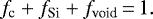
Figure 10 summarises the modelling results. Changes in Pr of the dust particles with regard to their porosity and wavelengths are shown. Black (grey) symbols indicate the modelled results with a mixture of 75 (65) vol.% of amorphous carbon and 25 (35) vol.% of silicate. To minimise effects from the resonant oscillations of monomers typical of X ~1 and from the absence of possibly smaller-sized monomers than applied in computation here, we mainly considered the longward end of the wavelength range we covered (7000–9000 Å). Additionally, the approximated nature of the dust (e.g. non-hierarchical structure without the surface roughness) could reduce the accuracy of the estimation around the minimum polarisation degree and the inversion angle (e.g. Kolokolova et al. 2018), and indeed it produces an unlikely (i.e. too positive) P distribution in our simulation compared to the ordinary cometary dust. Hence, given that a general polarimetric phase curve of cometary dust in the NPB (0° –22°) is roughly symmetrical around the Pmin at αmin ~ 11° (Kiselev et al. 2015), we considered modelled data only on the left side of the curve (i.e. α = 1° –10°) to minimise the impact of our simple properties of the modelled dust. In order to see a general trend, we took a mean of the modelled Pr values over the considered α range and marked it as a filled circle. Their error bars denote the standard deviations of the Pr values.
Dust with a porosity of 60% shows the best compatibility among the three modelled dust particles to the observed neutral PC (Fig. 5) and the Pr values at the phase angles in 2016 February and March (Fig. 6), within the error bars. Overall, the more transparent the dust, the greater the difference in Pr according tothe change of porosity. For the low-porosity case (60%), the PC is not significantly different between the two modelled cases within the error bars, but the depth of the NPB for the transparent dust (grey symbols in Fig. 10) is shallower than the 67P observations. For the fluffy case (95%), the transparent dust shows a more negative Pr and steeper blue PC than the absorbing dust (black symbols in Fig. 10). The transparent dust shows either too shallow (for the 60% case with the average Pr of −0.2%) or too deep (for the 95% case with the average Pr of −3.4%) depth in the NPB compared to the observed values of 67P dust. The transparent dust of a 80% porosity (grey dashed lines in panel d) also showed a local deep of Pr at 8000 Å and large Pr difference between 7000 and 9000 Å, both of which are incompatible to our observed PC (Figs. 1–3). For these reasons, we only consider the latter (i.e. a mixture of 75 vol.% of amorphous carbon and 25 vol.% of Mg-rich silicate) in the following discussion. The Pr of dust with a porosity of 80% appears to extend towards a bit more negative side in the NPB, but it could still explain the observed PC reasonably well. The 95% dust porosity explains neither the neutral PC nor the Pr values of the observed results. As such, we conclude that the dust particles dominating around the end of the summer are consistent with dust agglomerate with a porosity of 60–80%, but with a better match on the 60%-end side. In the following, we use 60% as a representative porosity value of the dust particles, showing non-fragmentation behaviour (Hornung et al. 2016). The retrieved microporosity of the dust particles is lower than the macroscopic porosity of the 67P nucleus of 75–85% estimated by CONSERT (Kofman et al. 2015, 2020), 65–80% from the Rosetta/Radio Science Investigation (RSI) (Pätzold et al. 2019), and 70–75% from the Optical, Spectroscopic, and Infrared Remote Imaging System (OSIRIS) pre-perihelion observations (Jorda et al. 2016). The microporosity is also lower than the macroscopic surface porosity of 87% derived by the Hapke model (Fornasier et al. 2015).
The mean density of dust particles with a porosity of 60% is then
 (15)
(15)
We note that ρX and fX are the density and fractional volumes occupied by the component X, respectively, where X equals ‘c’ for amorphous carbon, ‘Si’ for Mg-rich silicates, and ‘void’ for the void between the constituent particles we constrained. By substituting ρ = 3360 kg m-3 for the used silicates7, 1435 kg m-3 for the amorphous carbon (Jäger et al. 1998), fc = 0.3, fSi = 0.1, and fvoid = 0.6 into the equations, we obtained the mean density of the agglomerate as  770 kg m-3. Although the exact value could be different for dust constructed more sophisticatedly, the estimated density here is undoubtedly higher than the bulk density of the 67P nucleus (535 ± 35 kg m-3; Jorda et al. 2016), but well consistent with that of compact particles detected by GIADA (785
 kg m-3; Fulle et al. 2017).
This type of dust particles is expected to be ubiquitous on the surfaces of short-period comets (Hadamcik & Levasseur-Regourd 2009), which would be the outcome of the perennial sintering process under solar radiation. The predominance of such processed compact particles then explains the absence of 10 μm silicate emission features of 67P dust coma (Hanner et al. 1985) based on the positive correlation between the dust porosity and the silicate emission excess (Kwon et al. 2021). In the context of dust evolution, the behaviours of 67P dust in the NPB present in this study would probably showcase the ongoing processing of the 67P surface relative to its last apparitions and other dynamic groups of comets.
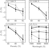 |
Fig. 10 Pr in the negative polarisation branch of the modelled dust aggregate having porosities of 60, 80, and 95% at the wavelengths of (a) 7000 Å, (b) 8000 Å, and (c) 9000 Å, and (d) the spectral dependence of Pr over the three wavelength domains. The results represent the mean Pr values and their standard deviations over the 1° –10° phase angle interval. Black (grey) symbols indicate the modelled results of the dust in the composition of 75 (65) vol.% amorphous carbon +25 (35) vol.% silicate. A more detailed description of the modelling is provided in the text. The Pr of the transparent dust at 9000 Å is −3.94 % and is not shown in this figure. |
4.2 Constraints on the amount of water ice in and the refractory-to-ice ratio of the compact dust particles
Although the dust activity level of 67P in early 2016 weakened significantly compared to its apex around the perihelion, the comet was still located inside the water frost line (rH = 2.7 au; Jewitt et al. 2007) so that the activity was discernible enough. The dust activity of the comet in this season was most likely driven by sublimation of water ice (Hansen et al. 2016). The heliocentric distance (rH ~ 2.5 au) at which we observed 67P is too large for organic materials to sublimate (usually at rH ≲ 0.7 au; Jones et al. 2018), but too small for bombarding solar wind particles to evaporate ice particles (significant at rH > 5 au; Mukai 1986), and for supervolatile ices (e.g. CO2 and CO) to lift off the constrained dust particles into the coma (Jewitt 2015). Frattin et al. (2017) suggest from the OSIRIS observationsthat the post-perihelion inner coma dust of 67P consists of three primary components – organics, silicates, and water ice. Aground-based observation with VLT/MUSE also corroborates the dust activity mainly driven by water-ice sublimation in early 2016 via clustering of the [OI] emission line at 6300 Å around the nucleus (Opitom et al. 2020).
The dust colour is the ratio of the intensity measured at two different wavelengths, thus it is able to trace the attributes of the dust particles. Although the Rosetta spacecraft was not equipped with a polarimeter, the dust colour measured at different positions in the coma by onboard instruments allows one to investigate the radial evolution of the dust properties in the coma of 67P. To this end, we utilised the Visible and Infrared Thermal Imaging Spectrometer (VIRTIS) spectroscopic data (Filacchione et al. 2020) and OSIRIS multi-band imaging data (Frattin et al. 2017) measured at 1.0–2.5 km and 80–437 km in cometocentric distance, respectively. Strictly speaking, our colour data are the integration of all signals within the 1000 km aperture, not the local signal at 1000 km. We could nonetheless assume thatour data well approximate the dust environment around 1000 km in radial distance, based on the following: (i) both the polarimetric and colour data stable against the effects induced by the near-nucleus outburst event in 2016 February (Grün et al. 2016) and (ii) apparently no changes over the two months indicating the sampling of the steady-state coma dust where the ejection information would have vanished out of the aperture.
We digitised the data points in panels b and d of Fig. 1 in Filacchione et al. (2020) and multiplied ten to match the unit. The data from Fig. 7 in Frattin et al. (2017) were obtained around UT 2016 January, yet they would not be problematic under the almost identical dust colour between January and March (Fig. 9a). The exact start and end wavelength positions of the blue and red sides are different between the observations: Filacchione et al. (2020) set 4000–5000 Å for the blue side and 5000–8000 Å for the red side, Frattin et al. (2017) set 4800–6490 Å for the blue side and 6490–8820 Å for the red side, and we set 4000–5500 Å and 5600–7900 Å for the blue and red sides, respectively. However, the spectral region where water ice shows its highest transparency (at ~4000–5000 Å; Mukai 1986; Warren 2019) is always covered by the blue sides of the observations, such that we could reliably monitor anycompositional variation induced by the water-ice sublimation. The change in the absorptivity of the mixture of the other two major materials (silicates and carbonaceous components) is continuous over 4000–9000 Å to a large extent (Dorschner et al. 1995; Kolokolova & Jockers 1997). The differences in α between the observations (on average ~90°, ~90°, and ~17° from inner to outer coma radius) would change the exact value of reddening. However, we expect that a weak (≲1%) dependence of the dust colour on the phase angle (Jewitt & Meech 1986; Gustafson & Kolokolova 1999; Kimura et al. 2003; Kolokolova et al. 2004; Bertini et al. 2017) keeps the observed reddening trend valid.
Figure 11 shows a synthesis of the spectral slopes in % (1000 Å)-1 measured atdifferent cometocentric distances. The reddening of the dust as it moves outwards from the nucleus is clearly shown. Provided that the colour changes the result from the changes in dust particles’ compositional and/or physical properties (Kolokolova et al. 2004), we could first rule out the latter effect since the Rosetta observations confirm the absence of any systematic shift of dust agglomerates into the smaller size distribution in the process of dust moving out of the nucleus at least in the <500 km distance range (Fulle et al. 2016; Frattin et al. 2021). Then, in terms of change in the dust composition, the observed trend in colour could support the sublimation of water-ice particles in the coma of 67P inferred from the Rosetta observations in early 2016. The different degree of reddening in the blue and red sides is also consistent with this scenario. All blue sides in Fig. 11 cover the 4000–5000 Å region (where the water ice has a minimum in the imaginary index of refraction); thus, it would be natural that the sublimation impact would be more significant therein than on the red side.
We performed an order-of-magnitude estimation to conjecture the possible amount of water ice embedded in the dust particles and therefrom their refractory-to-ice ratio. Most of the particles move radially from the nucleus (Frattin et al. 2021). For simplicity in the calculation, we assume that (i) the sublimation starts on ejection (0 km in altitude) and ends at 1000 km, which is roughly consistent with the observed central clustering of the intensity of the [OI] line (Opitom et al. 2020); (ii) water ice exists as pure one, which might be a proper treatment based on the Rosetta observations(e.g. Filacchione et al. 2016); and (iii) pure water ice and refractory dust do not coexist in thermal contact (Yang et al. 2009) such that the ice keeps its low temperature during sublimation. Given the velocity of 100 μm dust approximately of the order of 10 m s-1 (Fulle et al. 2010; Grün et al. 2016), it takes approximately 105 s to reach the endpoint. Any size of 1–1000 μm of pure ice might survive for the time at rH ~ 2.5 au (Mukai 1986). The rate of size decrease of the ice by sublimation can be expressed as
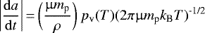 (17)
(17)
(Mukai & Schwehm 1981), where a is the radius of the dust particle, t is the time (105 s), μ is the mean molecular weight of water ice, mp is its atomic mass unit, ρ is the mass density of water ice (1000 kg m-3 is used), kB is the Boltzmann’s constant, and T is the water-ice temperature at the given heliocentric distance (~120 K for pure ice; Mukai 1986). The pv(T) means the saturated vapour pressure of the water ice at T for which we adopted the equation of Lamy (1974) that is valid at a low temperature of
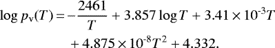 (18)
(18)
Substituting the values for pure water ice into Eqs. (17) and (18), the size of water ice for 105 s reduces by ~40 μm in linear dimension. Given that even the non-fragmenting dust agglomerates exhibit their inner structure quite well (Hornung et al. 2016), we assume that the water ice resides in the top 40 μm crust of the 100-μm-sized spherical dust agglomerate (the dust considered in Sect. 4.1). This results in the radius of an initially ejected dust particle (before sublimation) to be ~140 μm8. To make such dust plausible albedo-wise, by taking into account the volume fraction of ice abundance of the bright spots on the 67P surface on average of 4 vol.% (1–7.2 vol.%; Barucci et al. 2016), we further assume that 4% of the volume of the top crust consists of the ice particles. As a result, we obtain the volume fraction of water ice in the initially ejected dust as ~6% and their refractory-to-ice ratio of ~14. The dust density is then
 (19)
(19)

Here, fvoid, init denotes the initial void volume fraction (before sublimation), obtained by subtracting the ice fraction (fice) from the constrained porosity (0.6) in Sect. 4.1. We note that fc = 0.3 and fSi = 0.1 are used as in the previous section. The resultant ρinit is ~830 kg m-3. Since the volume of the dust particles is mostly occupied by refractory materials, the change of mechanical strength after the sublimation would be negligible (Haack et al. 2020). Assuming that the tensile strengths of water ice and organic materials in the dust are not significantly different from that of silicates (Gundlach et al. 2018; Bischoff et al. 2020), from Eq. (5) in Meisner et al. (2012), our filling factor of the dust upon ejection (1 − fvoid, init) corresponds to its tensile strength of ~8.2 kPa. This estimated tensile strength is much higher than the result of the dust showing catastrophic fragmentation patterns, but well consistent with the one of dust showing no or slight fragmentations in the collection of the COSIMA experiment (Hornung et al. 2016; Langevin et al. 2016).
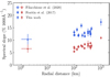 |
Fig. 11 Radial evolution of the spectral slope of the dust particles of 67P in % (1000 Å)-1. Circles indicate the average value of our three-epoch colour data (Fig. 9a). Blue and red symbols indicate spectral slopes measured at wavelengths shortward and longward of the inflection point. Horizontal error bars of triangles span the cometocentric distance (1.0–2.5 km) VIRTIS covered, while their vertical error bars denote the error of the weighted mean of observations (i.e. the standard deviation divided by the square root of the number of the data points) between UT2016 January and early March. |
5 Summary
We present new VLT spectropolarimetric observations of comet 67P/Churyumov-Gerasimenko obtained at the end of its intense southern summer. These datasets give us simultaneous polarimetric and colorimetric views at optical wavelengths. The main results of the analysis are as follows.
The Pr of 67P dust is positive at α = 26°.24 on UT 2016 January 12, and negative at α = 18°.47 and 5°.49 on UT 2016 February 04 and UT 2016 March 04, respectively, as expected from the observations of other cometary dust particles. Their wavelength dependences Pr(λ) over 4000–9000 Å are (0.14 ± 0.08)% (1000 Å)-1, (−0.03 ± 0.07)% (1000 Å)-1, and (0.03 ± 0.12)% (1000 Å)-1 for the three dates, which are much flatter than those of the dust of other comets, especially long-period comets and 2I/Borisov at similar observing geometries.
The trigonometric function describing the dependence of 67P dust’s Pr on the phase angle Pr(α) can be parameterised by b = 52.32 ± 20.87%, c1 = 1.01 ± 0.24, c2 = 9.99 ± 5.82, and α0 = 21°.71 ± 0°.51. The limited α coverage (<40°) and the small number of the available 67P data yields large errors of the fitting parameter b, which is relevant to the amplitude of the phase curve. The post-perihelion data of 67P dust appear more strongly polarised than pre-perihelion at α > 22°, but the number of pre-perihelion data sets is insufficient to make any firm conclusions. The depth of the NPB of 67P dust is slightly shallower than those of the long- and non-period comets, but comparable to other short-period comets.
The absolute value of the Pr at the given α in the NPB appears to decrease (i.e. a decrease in the depth of the NPB) between apparitions. The weighted mean of the Pr departure from the average trend is (−0.30 ± 0.10), (0.25 ± 0.13), and (0.46 ± 0.15)% for the 1983, 2009, and 2015 apparitions, respectively.
The 67P’s dust colour remains nearly constant over the two months in early 2016. It shows a red colour, with an inflection point around 5500 Å. The normalised spectral slopes of the shortward (blue side; 4000–5000 Å) and longward (red side; 5600–7900 Å) of the point are (17.3 ± 1.4) (1000 Å)-1 and (10.9 ± 0.6)% (1000 Å)-1, respectively. 67P during this term displays a slightly redder but overall consistent dust colour with the average of active Jupiter-family comets.
Our observations of 67P in early 2016 are compatible with the light scattering behaviour of the non-fragmenting dust agglomerates retrieved from the Rosetta observations. To estimate the plausible porosity of the dust, we constructed a simple light scattering model, setting a spherical dust aggregate particle of 100 μm in size. The dust consists of spherical monomers following a power-law size distribution with the differential index of −3 and the minimum and maximum sizes of 0.05 μm and 0.25 μm, respectively. Each monomer represents one type of composition, either amorphous carbon or silicate, constituting 75 vol.% and 25 vol.% in refractory materials, respectively. The dust porosity of ~60% shows the best match with our polarimetric results. We also tested a dust mixture of 65 vol.% of amorphous carbon and 35 vol.% of silicate, but its polarimetric properties are found to be inconsistent with the observed PC and Pr of 67P dust. The resultant density is ~770 kg m-3, which is higher than the bulk density of the 67P nucleus but consistent with the density of compact particles detected by the GIADA experiment.
Compiling the colour data obtained from the Rosetta (VIRTIS and OSIRIS) and our ground-based observations in early 2016, we found the signature of water-ice sublimation and the ensuing reddening of the dust colour as the radial distance increases. From an order-of-magnitude estimation, the volumeratio of water ice embedded in the dust particles before sublimation is expected to be ~6%, yielding the refractory-to-ice volume ratio of the dust as ~14. Consequently, its density and tensile strength would be ~830 kg m-3 and ~8.2 kPa, respectively. The retrieved tensile strength is consistent with the one derived from the dust particles showing no or slight fragmentation patterns in the COSIMA collection.
The observations presented here suggest the great potential of polarimetry as a tool to constrain physical properties of cometary dust and examine any differences therein between less-altered non- and long-period comets and relatively sintered short-period comets. We anticipate that this observing mode would help characterise dust profiles of a large number of comets in the years to come, especially for which only ground-based observations are available.
Acknowledgements
We thank Gianrico Filacchione and Elisa Frattin for providing the Rosetta VIRTIS and OSIRIS points in Fig. 11. YGK gratefully acknowledges the support of the Alexander von Humboldt Foundation. J.A. acknowledges funding by the Volkswagen Foundation. J.A. and J.M. acknowledge funding from the European Union’s Horizon 2020 research and innovation programme under grant agreement No 75390 CAstRA. A.C.L.R. acknowledges support from the French Space Agency (CNES), in relation with Rosetta and Comet Interceptor missions. C.S. acknowledges funding from the UK STFC, grants ST/L004569/1 and ST/V000586/1. This study is based on observations collected at the European Southern Observatory under ESO programme 096.C-0821.
Appendix A The extracted instrumental spectra of 67P with different aperture sizes
The extracted 16 light elements on each epoch were summed to retrieve Stokes I using Eq. 3. In six different aperture sizes applied, each light component and synthesised Stokes I show no radial variations in either the count or spectral shape throughout the observations. Figs. A.1–A.3 present I measured at 1,000 km and 7,500 km (panel (a)) and their differences (panel (b)) for the January, February, and March observations, respectively.Black (1,000 km aperture size) and grey (7,500 km aperture size) lines were overlapped, making their differences (Δ) almost zero. The larger the aperture sizes, the more significant error becomes due to the enhanced background noise. Thus, we decided to make use of the spectrum extracted with the 1,000-km-sized aperture for the observations at all observing epochs.
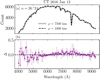 |
Fig. A.1 Counts of 67P dust extracted with the aperture sizes corresponding to 1,000 km (black) and 7,500 km (grey) in the cometocentric distance (a) and their differences (b) as a function of wavelength on UT 2016 January 12. We note that α indicates the phase angle on the epoch. In panel (a), black and grey lines overlap and they are indistinguishable from visual inspection. |
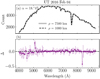 |
Fig. A.2 Same as Figure A.1, but on UT 2016 February 04. Black and grey lines overlap with each other. |
References
- Agarwal, J., A’Hearn, M. F., Vincent, J.-B., et al. 2016, MNRAS, 462, S78 [Google Scholar]
- A’Hearn, M. A. 1984, AJ, 89, 579 [CrossRef] [Google Scholar]
- Bagnulo, S., Landolfi, M., Landstreet, J. D., et al. 2009, PASP, 121, 993 [Google Scholar]
- Bagnulo, S., Cox, N. L. J., Cikota, A., et al. 2017, A&A, 608, 146 [Google Scholar]
- Bagnulo, S., Cellino, A., Kolokolova, L., et al. 2021, Nat. Commun., 12, 1797 [NASA ADS] [CrossRef] [Google Scholar]
- Bardyn, A., Baklouti, D., Cottin, H., et al. 2017, MNRAS, 469, S712 [NASA ADS] [CrossRef] [Google Scholar]
- Barucci, M. A., Filacchione, G., Fornasier, S., et al. 2016, A&A, 595, A102 [NASA ADS] [CrossRef] [EDP Sciences] [Google Scholar]
- Bentley, M. S., Schmied, R., Mannel, T., et al. 2016, Nature, 537, 73 [Google Scholar]
- Bertini, I., La Forgia, F., Tubiana, C., et al. 2017, MNRAS, 469, S404 [NASA ADS] [CrossRef] [Google Scholar]
- Bertini, I., La Forgia, F., Fulle, M., et al. 2019, MNRAS, 482, 2924 [Google Scholar]
- Biele, J., Ulamec, S., Maibaum, M., et al. 2015, Science, 349, aaa9816 [Google Scholar]
- Bischoff, D., Kreuzig, C., Haack, D., Gundlach, B., & Blum, J. 2020, MNRAS, 497, 2517 [CrossRef] [Google Scholar]
- Boehnhardt, H., Riffeser, A., Kluge, M., et al. 2016, MNRAS, 462, 376 [Google Scholar]
- Bohren, C., & Huffman, D. 1983, Absorption and Scattering of Light by Small Particles (New York: Wiley Sons) [Google Scholar]
- Chernova, G. P., Kiselev, N. N., & Jockers, K. 1993, Icarus, 103, 144 [Google Scholar]
- Cikota, A., Patat, F., Cikota, S., & Faran, T. 2017, MNRAS, 464, 4146 [Google Scholar]
- Datson, J., Flynn, C., & Portinari, L. 2015, A&A, 574, A124 [NASA ADS] [CrossRef] [EDP Sciences] [Google Scholar]
- Della Corte, V., Rotundi, A., Fulle, M., et al. 2015, A&A, 583, A13 [NASA ADS] [CrossRef] [EDP Sciences] [Google Scholar]
- Dorschner, J., Begemann, B., Henning, T., Jäger, C., & Mutschke, H. 1995, A&A, 300, 503 [NASA ADS] [Google Scholar]
- Emery, J. 2002, PhD Thesis, The University of Arizona, USA [Google Scholar]
- Filacchione, G., De Sanctis, M. C., Capaccioni, F., et al. 2016, Nature, 529, 368 [NASA ADS] [CrossRef] [Google Scholar]
- Filacchione, G., Capaccioni, F., Ciarniello, M., et al. 2020, Nature, 578, 49 [NASA ADS] [CrossRef] [Google Scholar]
- Fornasier, S., Hasselmann, P., Barucci, M. A., et al. 2015, A&A, 583, A30 [NASA ADS] [CrossRef] [EDP Sciences] [Google Scholar]
- Fulle, M., Colangeli, L., Agarwal, J., et al. 2010, A&A, 522, A63 [NASA ADS] [CrossRef] [EDP Sciences] [Google Scholar]
- Fulle, M., Altobelli, N., Buratti, B., et al. 2016, MNRAS, 462, 2 [Google Scholar]
- Fulle, M., Della Corte, V., Rotundi, A., et al. 2017, MNRAS, 469, S45 [Google Scholar]
- Fulle, M., Blum, J., Rotundi, A., et al. 2020, MNRAS, 493, 4039 [CrossRef] [Google Scholar]
- Frattin, E., Cremonese, G., Simioni, E., et al. 2017, MNRAS, 469, S195 [NASA ADS] [CrossRef] [Google Scholar]
- Frattin, E., Bertini, I., Ivanovski, S. L., et al. 2021, MNRAS, 504, 4687 [NASA ADS] [CrossRef] [Google Scholar]
- Grün, E., Agarwal, J., Altobelli, N., et al. 2016, MNRAS, 462, S220 [CrossRef] [Google Scholar]
- Gundlach, B., Schmidt, K. P., Kreuzig, C., et al. 2018, MNRAS, 479, 1273 [NASA ADS] [CrossRef] [Google Scholar]
- Gundlach, B., Fulle, M., & Blum, J. 2020, MNRAS, 493, 3690 [NASA ADS] [CrossRef] [Google Scholar]
- Gustafson, B. Å. S., & Kolokolova, L. 1999, J. Geophys. Res., 104, 31711 [CrossRef] [Google Scholar]
- Güttler, C., Mannel, T., Rotundi, A., et al. 2019, A&A, 24, 1 [Google Scholar]
- Haack, D., Otto, K., Gundlach, B., et al. 2020, A&A, 642, A218 [NASA ADS] [CrossRef] [EDP Sciences] [Google Scholar]
- Hadamcik, E., & Levasseur-Regourd, A. C. 2003a, J. Quant. Spectr. Rad. Transf., 79, 661 [Google Scholar]
- Hadamcik, E., & Levasseur-Regourd, A. C. 2003b, A&A, 403, 757 [NASA ADS] [CrossRef] [EDP Sciences] [Google Scholar]
- Hadamcik, E., & Levasseur-Regourd, A. C. 2009, P&SS, 57, 1118 [NASA ADS] [CrossRef] [Google Scholar]
- Hadamcik, E., Sen, A. K., Levasseur-Regourd, A. C., Gupta, R., & Lasue, J. 2010, A&A, 517, A86 [NASA ADS] [CrossRef] [EDP Sciences] [Google Scholar]
- Hadamcik, E., Levasseur-Regourd, A. C., Hines, D. C., et al. 2016, MNRAS, 462, 507 [Google Scholar]
- Hanner, M. S., Tedesco, E., Tokunaga, A. T., et al. 1985, Icarus, 64, 11 [Google Scholar]
- Hansen, K. C., Altwegg, K., Berthelier, J.-J., et al. 2016, MNRAS, 462, S491 [Google Scholar]
- Hornung, K., Merouane, S., Hilchenbach, M., et al. 2016, P&SS, 133, 63 [NASA ADS] [CrossRef] [Google Scholar]
- Ivanova, O., Rosenbush, V., Kiselev, N., Afanasiev, V., & Korsun, P. 2017, MNRAS, 469, 386 [Google Scholar]
- Jäger, C., Mutschke, H., & Henning, T. 1998, A&A, 332, 291 [NASA ADS] [Google Scholar]
- Jewitt, D. 2015, AJ, 150, 201 [NASA ADS] [CrossRef] [Google Scholar]
- Jewitt, D., & Meech, K. J. 1986, AJ, 310, 937 [NASA ADS] [CrossRef] [Google Scholar]
- Jewitt, D., Chizmadia, L., Grimm, R., & Prialnik, D. 2007, in Protostars and Planets V, eds. V. B. Reipurth, D. Jewitt, K. Keil (Tucson: University of Arizona Press), 863 [Google Scholar]
- Jones, G. H., Knight, M. M., Battams, K., et al. 2018, Space Sci. Rev., 214, 20 [NASA ADS] [CrossRef] [Google Scholar]
- Jorda, L., Gaskell, R., Capanna, C., et al. 2016, Icarus, 277, 257 [Google Scholar]
- Kikuchi, S. 2006, J. Quant. Spectr. Rad. Transf., 100, 179 [NASA ADS] [CrossRef] [Google Scholar]
- Kimura, H., Kolokolova, L., & Mann, I. 2003, A&A, 407, L5 [NASA ADS] [CrossRef] [EDP Sciences] [Google Scholar]
- Kimura, H., Kolokolova, L., & Mann, I. 2006, A&A, 449, 1243 [NASA ADS] [CrossRef] [EDP Sciences] [Google Scholar]
- Kiselev, N., & Velichko, F. 1996, EM&P, 78, 347 [Google Scholar]
- Kiselev, N., Rosenbush, V., Kolokolova, L., & Levasseur-Regourd, A. C. 2015, in Polarimetry of Stars and Planetary Systems, eds. L. Kolokolova, J. Hough, & A. C. Levasseur-Regourd (Cambridge: Cambridge University Press), 379 [CrossRef] [Google Scholar]
- Kiselev, N., Shubina, E., Velichko, S., et al. 2017, Compilation of Comet Polarimetry from Published and Unpublished Sources, urn:nasa:pds:compil-comet:polarimetry::1.0, NASA Planetary Data System [Google Scholar]
- Kofman, W., Herique, A., Barbin, Y., et al. 2015, Science, 349, 6247 [CrossRef] [Google Scholar]
- Kofman, W., Zine, S., Herique, A., et al. 2020, MNRAS, 497, 2616 [NASA ADS] [CrossRef] [Google Scholar]
- Kolokolova, L., & Jockers, K. 1997, PSS, 45, 1543 [NASA ADS] [Google Scholar]
- Kolokolova, L., Jockers, K., Chernova, G., & Kiselev, N. 1997, Icarus, 126, 351 [NASA ADS] [CrossRef] [Google Scholar]
- Kolokolova, L., Jockers, K., Gustafson, B. Å, S., & Lichtenberg, G. 2001, J. Quant. Spectr. Rad. Transf., 106, 10113 [Google Scholar]
- Kolokolova, L., Hanner, M. S., Levasseur-Regourd, A. C., & Gustafson, B. Å. S. 2004, in Comets II, eds. M. Festou, H. U. Keller, & H. A. Weaver (Tucson: University of Arizona Press), 577 [Google Scholar]
- Kolokolova, L., Das, H. S., Dubovik, O., Lapyonok, T., & Yang, P. 2015, P&SS, 116, 30 [NASA ADS] [CrossRef] [Google Scholar]
- Kolokolova, L., Nagdimunov, L., & Mackowski, D. 2018, J. Quant. Spectr. Rad. Transf., 204, 138 [NASA ADS] [CrossRef] [Google Scholar]
- Knight, M. M., Snodgrass, C., Vincent, J.-B., et al. 2017, MNRAS, 469, 661 [Google Scholar]
- Kwon, Y. G., Ishiguro, M., Shinnaka, Y., et al. 2018, A&A, 620, A161 [EDP Sciences] [Google Scholar]
- Kwon, Y. G., Ishiguro, M., Kwon, J., et al. 2019, A&A, 629, A121 [EDP Sciences] [Google Scholar]
- Kwon, Y. G., Kolokolova, L., Agarwal, J., & Markkanen, J. 2021, A&A, 650, L7 [NASA ADS] [CrossRef] [EDP Sciences] [Google Scholar]
- Lamy, P. L. 1974, A&A, 35, 197 [NASA ADS] [Google Scholar]
- Langevin, Y.. Hilchenbach, M., Ligier, N., et al. 2016, Icarus, 271, 76 [CrossRef] [Google Scholar]
- Lasue, J., Levasseur-Regourd, A. C., Hadamcik, E., & Alcouffe, G. 2009, Icarus, 199, 129 [NASA ADS] [CrossRef] [Google Scholar]
- Levasseur-Regourd, A. C., Agarwal, J., Cottin, H., et al. 2018, Space Sci. Rev., 214, 64 [NASA ADS] [CrossRef] [Google Scholar]
- Longobardo, A., Della Corte, V., Rotundi, A. et al. 2016 MNRAS, 496, 125 [Google Scholar]
- Lumme, K., & Muinonen, K. 1993, Asteroids, Comets, Meteors, IAU Symp., 160, 194 [NASA ADS] [Google Scholar]
- Meisner, T., Wurm, G., & Teiser, J. 2012, A&A, 544, A138 [NASA ADS] [CrossRef] [EDP Sciences] [Google Scholar]
- Mann, I., Kimura, H., & Kolokolova, L. 2004, J. Quant. Spectr. Rad. Transf., 89, 291 [NASA ADS] [CrossRef] [Google Scholar]
- Mannel, T., Bentley, M. S., Schmied, R., et al. 2016, MNRAS, 462, S304 [NASA ADS] [CrossRef] [Google Scholar]
- Mannel, T., Bentley, M. S., Boakes, P. D., et al. 2019, A&A, 630, A26 [NASA ADS] [CrossRef] [EDP Sciences] [Google Scholar]
- Marschall, R., Skorov, Y., Zakharov, V., et al. 2020, Space Sci. Rev., 216, 130 [Google Scholar]
- Markkanen, J., & Agarwal, J. 2020, A&A, 643, A16 [NASA ADS] [CrossRef] [EDP Sciences] [Google Scholar]
- Mottola, S., Arnold, G., Grotheus, H.-G., et al. 2015, Science, 349, aab0232 [CrossRef] [Google Scholar]
- Muinonen, K., Penttila, A., & Videen, G. 2015, in Polarimetry of Stars and Planetary Systems, eds. L. Kolokolova, J. Hough, & A. C. Levasseur-Regourd (Cambridge: Cambridge University Press), 114 [CrossRef] [Google Scholar]
- Muinonen, K., Markkanen, J., Väisänen, Peltoniemi, J., & Penttilä, A. 2018, Opt. Lett., 43, 683 [NASA ADS] [CrossRef] [Google Scholar]
- Mukai, T. 1986, A&A, 164, 397 [NASA ADS] [Google Scholar]
- Mukai, T., & Schwehm, G. 1981, A&A, 95, 373 [NASA ADS] [Google Scholar]
- Myers, R. V., & Nordsieck, K. H. 1984, Icarus, 58, 431 [NASA ADS] [CrossRef] [Google Scholar]
- Opitom, C., Snodgrass, C., Fitzsimmons, A., et al. 2017, MNRAS, 469, 222 [Google Scholar]
- Opitom, C., Guilbert-Lepoutre, A., Besse, S., Yang, B., & Snodgrass, C. 2020, A&A, 644, 143 [Google Scholar]
- Pajola, M., Lucchetti, A., Fulle, M., et al. 2017, MNRAS, 469, S636 [Google Scholar]
- Patat, F., Moehler, S., O’Brien, K., et al. 2011, A&A, 527, A91 [NASA ADS] [CrossRef] [EDP Sciences] [Google Scholar]
- Pätzold, M., Ander, T. P., Hahn, M., et al. 2019, MNRAS, 483, 2337 [CrossRef] [Google Scholar]
- Petrova, E. V., Jockers, K., & Kiselev, N. N. 2001, Space Sci. Rev., 35, 390 [Google Scholar]
- Preusker, F., Scholten, F., Matz, K., et al. 2017, A&A, 607, L1 [NASA ADS] [CrossRef] [EDP Sciences] [Google Scholar]
- Raponi, A., Ciarniello, M., Capaccioni, F., et al. 2020, Nat. Astron., 5, 500 [Google Scholar]
- Renard, J.-B., Hadamcik, E., & Levasseur-Regourd, A. C. 1996, A&A, 316, 263 [Google Scholar]
- Rosenbush, V., Ivanova, O., Kiselev, N., Kolokolova, L., & Afanasiev, V. 2017, MNRAS, 469, 475 [Google Scholar]
- Schleicher, D. 2006, Icarus, 181, 442 [CrossRef] [Google Scholar]
- Snodgrass, C., Opitom, C., De Val-Borro, M., et al. 2016, MNRAS, 462, 138 [Google Scholar]
- Snodgrass, C., A’Hearn, M. F., Aceituno, F., et al. 2017, Phil. Trans. R. Soc. London Ser. A, 375, 20160249 [Google Scholar]
- Solontoi, M., Ivezić, Ž., Jurić, M., et al. 2012, Icarus, 218, 571 [CrossRef] [Google Scholar]
- Spohn, T., Knollenber, J., Ball, A. J., et al. 2015, Science, 349, aab0464 [CrossRef] [Google Scholar]
- Stinson, A., Bagnulo, S., Tozzi, G. P., et al. 2016, A&A, 594, A110 [NASA ADS] [CrossRef] [EDP Sciences] [Google Scholar]
- Storrs, A., Cochran, A., & Barker, E. 1992, Icarus, 98, 163 [NASA ADS] [CrossRef] [Google Scholar]
- Thomas, N., Ulamec, S., Kührt, E., et al. 2017, Space Sci. Rev., 215, 47 [Google Scholar]
- van Dokkum, P. G. 2001, PASP, 113, 1420 [Google Scholar]
- Väisänen, T., Markkanen, J., Penttilä, A., & Muinonen, K. 2019, PloS one, 14, 1 [Google Scholar]
- Warren, S. 2019, Phil. Trans. R. Soc. A, 377, 20180161 [CrossRef] [Google Scholar]
- Yang, B., Jewitt, D., & Bus, S. J. 2009, AJ, 137, 4538 [NASA ADS] [CrossRef] [Google Scholar]
Obtained by Emery (2002) using the compositional information from Dorschner et al. (1995).
If the ice-bearing constituents have an intimate mixture of ice and refractories in noticeable thermal contact, unlike assumptions herein, then the resultant size of the dust particles needs to be centimetre-sized or larger (Mukai 1986; Markkanen & Agarwal 2020).
All Tables
All Figures
|
Fig. 1 Sky images of 67P obtained from a single exposure. The phase angle and equivalent filter range are provided on top of each figure. Panel awas obtained with a 120-s exposure, while panels b and cwere obtained with a 60-s exposure. Panels a and b cover the FoV of 1′.0 × 1′.0, while panel cspans 2′.0 × 1′.2 to encompass the neck-line structure. North is up and east is to the left. The level of brightness was inverted and arbitrarily adjusted to enhance weak coma structures. The 1000-km-sized aperture applied in this study is overlaid as a magenta box, covering the inner coma part. The solid and dashed arrows denote the Sun–comet radius vectors and the comet’s negative heliocentric velocity vectors, respectively. Background structures are either stars or cosmic rays. |
| In the text | |
|
Fig. 2 Pr of 67P dust in % (a) and the mean and 1σ error of the position angle of Pr with regard to the scattering plane (θr) as a functionof the wavelength (b) observed at α = 26°.4 on UT 2016 January 12. The black points in panel a were binned to have wavelength intervals of ~52 Å. The large error bars result from the remnants of the skylines that were not perfectly subtracted due to the limited slitwidth. The red solid and upper and lower dashed lines inpanel b indicate the weighted mean of θr (θr, avg) and its error(the standard deviation divided by the square of the number of the data points), respectively. The black line marks θr = 0°, the expected value when the dust is distributed randomly in the coma. |
| In the text | |
|
Fig. 3 Same as Fig. 2, but at α = 18°.47 on UT 2016 February 04. The black line indicates θr = 90°, the expected value when the dust is distributed randomly in the coma. |
| In the text | |
|
Fig. 4 Same as Fig. 2, but at α = 5°.49 on UT 2016 March 04. The black line indicates θr = 90°, the expected value when the dust is distributed randomly in the coma. |
| In the text | |
|
Fig. 5 Polarimetric colour (PC) of comets over the α range of 0° –35°. All data points except 67P in this study are quoted from the NASA/PDS comet polarimetric archive (Kiselev et al. 2017) and from Bagnulo et al. (2021). Panels a and b present the data in pre-perihelion (180° < ν < 350°, where ν means the true anomaly) and post-perihelion (10° < ν ≤ 180°), respectively. There are no available points around the perihelion (350° ≤ ν ≤ 10°). Red circles of 67P are obtained from the least-square linear fit of 67P dust (Figs. 2–4), and their error bars indicate 1σ uncertainties of the fitting. Black open symbols were derived from the comet data observed by aperture polarimetric observations. Thus, the error bars of their PCs were derived from the error propagation of Pr values measured at discrete wavelength points. ‘Garradd’ and ‘LINEAR’ denote comets C/2009 P1 (Garradd) and C/2000 WM1 (LINEAR), respectively. |
| In the text | |
|
Fig. 6 Polarisation of 67P dust versus phase angle. Open and filled symbols denote the pre- and post-perihelion data, respectively. Black symbols are the archival data (Kiselev et al. 2017) where different shapes indicate the datasets obtained by different works: circle (Myers & Nordsiseck 1984), square (Hadamcik et al. 2016), triangle (Hadamcik et al. 2010), polygon (Stinson et al. 2016), and diamond (Rosenbush et al. 2017). Red diamonds denote our spectropolarimetric data. Background grey symbols (Kiselev et al. 2017) are excluded from the analysis due to the significant difference in the aperture sizes from ours. The solid and dashed curves indicate the average dependence derived from Eq. (11) for the data as a whole and in post-perihelion, respectively. The best-fit parameters of the curves are provided in the text. |
| In the text | |
|
Fig. 7 Departure of the Pr of 67P dust in each apparition from to the average trend. The black fitting line in Fig. 6 now corresponds to the horizontal dashed lines at ΔPr = 0. The horizontal solid lines and shaded areas denote the weighted mean and error, in which the colour scheme follows the symbols in the legend. Open and filled symbols denote the pre- and post-perihelion data of 67P dust. Only post-perihelion data were used to estimate ΔPr. |
| In the text | |
|
Fig. 8 Polarisation of all available comets’ dust versus phase angle. The black solid line and shaded areas denote the average trend of the dependence and its 3σ error, respectively. As in Fig. 6, open and filled symbols denote the pre- and post-perihelion data, while background grey circles represent data points discarded from the fitting because of either their large aperture size (≫10 000 km in cometocentric distance) and/or the possible gas contamination. All symbols are the archival data of Kiselev et al. (2017), except for the four points of 2I/Borisov (Bagnulo et al. 2021) and three points of 67P (this study). We exclude unique comets C/1995 O1 (Hale-Bopp) and 2I/Borisov from the fitting, since their Pr has been found to be significantly higher. The red diamonds edged with black lines are our spectropolarimetric data. The best fit parameters of the fitted curve are b = 25.69 ± 1.27%, c1 = 0.67 ± 0.02, c2 = (1.54 ± 0.85) × 10-13, and α0 = 21°.25 ± 0°.14. A detailed description of the legend is provided in the text. |
| In the text | |
|
Fig. 9 Relative brightness of 67P dust normalised at 5500 Å. (a) The dust colour slopes (Eq. (14)) are shown as the solid lines with 3σ fitting errors in grey regions. (b) Two solid black lines indicate the lower (5 ± 2% (1000 Å)-1) and upper (18 ± 2% (1000 Å)-1) reflectivity limits of the dust of nine comets over 3500–6500 Å, respectively (Jewitt & Meech 1986). The thick grey solid and dashed lines indicate the average reflectivity trend and standard deviation of 31 active comets (8.4 ± 3.6% (1000 Å)-1) over 3540–9050 Å used in Solontoi et al. (2012). |
| In the text | |
|
Fig. 10 Pr in the negative polarisation branch of the modelled dust aggregate having porosities of 60, 80, and 95% at the wavelengths of (a) 7000 Å, (b) 8000 Å, and (c) 9000 Å, and (d) the spectral dependence of Pr over the three wavelength domains. The results represent the mean Pr values and their standard deviations over the 1° –10° phase angle interval. Black (grey) symbols indicate the modelled results of the dust in the composition of 75 (65) vol.% amorphous carbon +25 (35) vol.% silicate. A more detailed description of the modelling is provided in the text. The Pr of the transparent dust at 9000 Å is −3.94 % and is not shown in this figure. |
| In the text | |
|
Fig. 11 Radial evolution of the spectral slope of the dust particles of 67P in % (1000 Å)-1. Circles indicate the average value of our three-epoch colour data (Fig. 9a). Blue and red symbols indicate spectral slopes measured at wavelengths shortward and longward of the inflection point. Horizontal error bars of triangles span the cometocentric distance (1.0–2.5 km) VIRTIS covered, while their vertical error bars denote the error of the weighted mean of observations (i.e. the standard deviation divided by the square root of the number of the data points) between UT2016 January and early March. |
| In the text | |
|
Fig. A.1 Counts of 67P dust extracted with the aperture sizes corresponding to 1,000 km (black) and 7,500 km (grey) in the cometocentric distance (a) and their differences (b) as a function of wavelength on UT 2016 January 12. We note that α indicates the phase angle on the epoch. In panel (a), black and grey lines overlap and they are indistinguishable from visual inspection. |
| In the text | |
|
Fig. A.2 Same as Figure A.1, but on UT 2016 February 04. Black and grey lines overlap with each other. |
| In the text | |
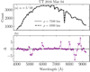 |
Fig. A.3 Same as Figure A.1, but on UT 2016 March 04. Black and grey lines overlap with each other. |
| In the text | |
Current usage metrics show cumulative count of Article Views (full-text article views including HTML views, PDF and ePub downloads, according to the available data) and Abstracts Views on Vision4Press platform.
Data correspond to usage on the plateform after 2015. The current usage metrics is available 48-96 hours after online publication and is updated daily on week days.
Initial download of the metrics may take a while.