| Issue |
A&A
Volume 656, December 2021
|
|
|---|---|---|
| Article Number | A162 | |
| Number of page(s) | 25 | |
| Section | Stellar atmospheres | |
| DOI | https://doi.org/10.1051/0004-6361/202141980 | |
| Published online | 16 December 2021 | |
The CARMENES search for exoplanets around M dwarfs
Stellar atmospheric parameters of target stars with STEPARSYN★
1
Departamento de Física de la Tierra y Astrofísica & IPARCOS-UCM (Instituto de Física de Partículas y del Cosmos de la UCM), Facultad de Ciencias Físicas, Universidad Complutense de Madrid,
28040
Madrid,
Spain
e-mail: This email address is being protected from spambots. You need JavaScript enabled to view it.
2
Centro de Astrobiología (CSIC-INTA), ESAC, Camino Bajo del Castillo s/n,
28691
Villanueva de la Cañada,
Madrid,
Spain
3
Centro de Astrobiología (CSIC-INTA),
Carretera a Ajalvir km 4,
28850
Torrejón de Ardoz,
Madrid,
Spain
4
Instituto de Astrofísica e Ciências do Espaço, Universidade do Porto, CAUP, Rua das Estrelas,
4150-762
Porto,
Portugal
5
Instituto de Astrofísica de Canarias,
c/ Vía Láctea s/n,
38205
La Laguna,
Tenerife,
Spain
6
Universidad de La Laguna,
Departamento de Astrofísica,
38206
La Laguna,
Tenerife,
Spain
7
Hamburger Sternwarte,
Gojenbergsweg 112,
21029
Hamburg,
Germany
8
Thüringer Landessternwarte Tautenburg,
Sternwarte 5,
07778
Tautenburg,
Germany
9
Homer L. Dodge Department of Physics and Astronomy, University of Oklahoma,
440 West Brooks Street, Norman,
OK-73019
Oklahoma,
USA
10
Institut de Ciències de l’Espai (CSIC),
Campus UAB, c/ de Can Magrans s/n,
08193
Cerdanyola del Vallès,
Spain
11
Institut d’Estudis Espacials de Catalunya (IEEC),
c/ Gran Capità 2-4,
08034
Barcelona,
Spain
12
Institut für Astrophysik, Georg-August-Universität-Göttingen,
Friedrich-Hund-Platz 1,
37077
Göttingen,
Germany
13
Landessternwarte, Zentrum für Astronomie der Universität Heidelberg,
Königstuhl 12,
69117
Heidelberg,
Germany
14
Instituto de Astrofísica de Andalucía (IAA-CSIC),
Glorieta de la Astronomía s/n,
18008
Granada,
Spain
15
Observatorio de Calar Alto, Sierra de los Filabres,
04550
Gérgal, Almería,
Spain
16
Max-Planck-Institut für Astronomie,
Königstuhl 17,
69117
Heidelberg,
Germany
17
Max-Planck-Institut für Sonnensystemforschung,
Justus-von- Liebig-Weg 3,
37077
Göttingen,
Germany
18
Department of Physics, University of Warwick,
Gibbet Hill Road,
Coventry
CV4 7AL,
UK
Received:
6
August
2021
Accepted:
7
October
2021
Abstract
We determined effective temperatures, surface gravities, and metallicities for a sample of 343 M dwarfs observed with CARMENES, the double-channel, high-resolution spectrograph installed at the 3.5 m telescope at Calar Alto Observatory. We employed STEPARSYN, a Bayesian spectral synthesis implementation particularly designed to infer the stellar atmospheric parameters of late-type stars following a Markov chain Monte Carlo approach. We made use of the BT-Settl model atmospheres and the radiative transfer code turbospectrum to compute a grid of synthetic spectra around 75 magnetically insensitive Fe I and Ti I lines plus the TiO γ and ϵ bands. To avoid any potential degeneracy in the parameter space, we imposed Bayesian priors on Teff and logg based on the comprehensive, multi-band photometric data available for the sample. We find that this methodology is suitable down to M7.0 V, where refractory metals such as Ti are expected to condense in the stellar photospheres. The derived Teff, logg, and [Fe/H] range from 3000 to 4200 K, 4.5 to 5.3 dex, and −0.7 to 0.2 dex, respectively. Although our Teff scale is in good agreement with the literature, we report large discrepancies in the [Fe/H] scales, which might arise from the different methodologies and sets of lines considered. However, our [Fe/H] is in agreement with the metallicity distribution of FGK-type stars in the solar neighbourhood and correlates well with the kinematic membership of the targets in the Galactic populations. Lastly, excellent agreement in Teff is found for M dwarfs with interferometric angular diameter measurements, as well as in the [Fe/H] between the components in the wide physical FGK+M and M+M systems included in our sample.
Key words: techniques: spectroscopic / stars: fundamental parameters / stars: late-type / stars: low-mass
Full Tables B.1–B.3 are only available at the CDS via anonymous ftp to cdsarc.u-strasbg.fr (130.79.128.5) or via http://cdsarc.u-strasbg.fr/viz-bin/cat/J/A+A/656/A162
© ESO 2021
1 Introduction
M dwarfs are cool and faint stars that comprise about two-thirds of the stellar population in the solar neighbourhood (Henry et al. 2018; Reylé et al. 2021). With main-sequence lifespans longer than the age of the Universe (Laughlin et al. 1997), these stars are not only an excellent record of the structure and evolution of the Milky Way (Bochanski et al. 2007), but have also become prime targets for exoplanet surveys owing to their low mass, low temperature, and ubiquity (Bonfils et al. 2013; Dressing & Charbonneau 2013; Reiners et al. 2018); this combination favours detections of Earth-mass planets inside their habitable zone, where liquid water can be sustained (Scalo et al. 2007).
Installed at the 3.5 m telescope at the Calar Alto Observatory, the CARMENES instrument (Quirrenbach et al. 2020)is, along with SPIRou (Donati et al. 2020), NIRPS (Wildi et al. 2017), HPF (Mahadevan et al. 2012), IRD (Kotani et al. 2018), MAROON-X (Seifahrt et al. 2020), NEID (Schwab et al. 2016), and GIARPS (Claudi et al. 2018), a new-generation spectrograph designed to detect Earth-mass planets around M dwarfs by means of the radial velocity technique (Reiners et al. 2018). It consists of optical (hereafter VIS) and near-infrared (NIR) channels that cover the 5200–9600 Å and 9600–17100 Å wavelength regions with spectral resolutions of R = 94 600 and R = 80 400, respectively.As of mid-2020, the CARMENES exoplanet survey had collected more than 18 500 VIS and 18 000 NIR spectra for a sample of 365 M dwarfs (Quirrenbach et al. 2020) obtained as part of its 750-night guaranteed time observations(GTO) programme. In addition to detecting and characterising the orbits of exoplanets (e.g. Trifonov et al. 2018, 2020; Luque et al. 2019; Zechmeister et al. 2019) and their atmospheres (Nortmann et al. 2018; Alonso-Floriano et al. 2019; Yan et al. 2019), the survey represents a unique opportunity to gain insights into the nature of M dwarfs (namely, their photospheric parameters, chemical compositions, magnetic fields, and chromospheric activity levels) in a statistically relevant way (Fuhrmeister et al. 2018, 2020; Passegger et al. 2018, 2019; Hintz et al. 2019, 2020; Schöfer et al. 2019; Schweitzer et al. 2019; Shulyak et al. 2019; Abia et al. 2020; Shan et al. 2021).
In the context of exoplanet research, a thorough account of the general properties of host stars directly affects the determination of the position of the habitable zone (Selsis et al. 2007; Kopparapu et al. 2013), the radius and mass of detected exoplanets, and their composition (Maldonado et al. 2020; Ishikawa et al. 2020). In addition, planet formation theories attempt to explain the observed occurrence rate of exoplanets (Johnson et al. 2010; Howard et al. 2012; Buchhave et al. 2012; Sabotta et al. 2021) and selection effects (Winn & Fabrycky 2015) in terms of the stellar parameters.
However, the computation of photospheric parameters for M dwarfs from stellar spectra, namely the effective temperature, Teff, surface gravity, logg, and stellar metallicity, [Fe/H], is an arduous challenge. The low photospheric temperatures give rise to pervasive molecular bands that severely distort the stellar continuum (Kirkpatrick et al. 1991; Tinney & Reid 1998; Reiners et al. 2018). This alone rules out classical techniques commonly adopted in the analysis of solar-type spectra, such as the equivalent width (EW) method (Marfil et al. 2020). Stellar convection in M dwarfs also calls into question some of the physical assumptions behind the model atmospheres of late-type stars, such as local thermodynamic equilibrium (LTE) and one-dimensional (1D) geometry for radiative transfer, which often represents a limitation to the interpretation at the resolution achieved by modern spectrographs (Bergemann et al. 2017; Olander et al. 2021). Furthermore, M dwarfs may exhibit strong magnetic fields that not only drive stellar activity (Delfosse et al. 1998; Donati et al. 2008), but may also distort magnetically sensitive lines via the Zeeman effect (Landi Degl’Innocenti & Landolfi 2004; Passegger et al. 2019). It is, therefore, difficult to choose a set of lines to disentangle the impact of the magnetic field and the photospheric parameters on the stellar spectra (Shulyak et al. 2019). To make matters worse, telluric absorption is ubiquitous in the NIR (Reiners et al. 2018; Nagel 2019), where the spectral energy distribution of M dwarfs peaks (Cifuentes et al. 2020).
Despite the above, several methods have proved fruitful for inferring Teff, log g, and [Fe/H] in M dwarfs, including spectral synthesis (e.g. Passegger et al. 2018, 2019; Rajpurohit et al. 2018b; Souto et al. 2020; Hejazi et al. 2020), pseudo-EWs (e.g. Mann et al. 2013a, 2014; Neves et al. 2014; Maldonado et al. 2015, 2020), and spectral indices (e.g. Rojas-Ayala et al. 2012; Khata et al. 2020), all of which can be further investigated following a machine-learning approach (e.g. Sarro et al. 2018; Antoniadis-Karnavas et al. 2020; Passegger et al. 2020; Li et al. 2021). In general terms, spectral synthesis relies on a minimisation algorithm to find the synthetic spectrum that best matches the observed spectrum (Valenti & Fischer 2005; Brewer et al. 2016), while pseudo-EW and spectral index approaches draw on the sensitivity of certain features to Teff and [Fe/H], as well as on calibrations with wide physical binaries harbouring an FGK-type primary with known metallicity (Casagrande et al. 2008; Neves et al. 2012; Montes et al. 2018, and references therein). Further studies have focused on ensuring consistency between these two approaches (Veyette et al. 2017).
Semi-empirically calibrated methods have been widely adopted in the literature. For example, based on observations in the photometric Y band (9470–11 210 Å) with NIRSPEC on Keck II, Veyette et al. (2017) used a method to derive Teff, [Fe/H], and [Ti/H] that rests on the approach described by Mann et al. (2013b) and a calibration sample of M dwarfs in common proper motion FGK+M binaries from Mann et al. (2013a). The method relies on the measured FeH index in the Wing-Ford band and on the EWs of seven Fe I and ten Ti I lines found in the Y band. More recently, Maldonado et al. (2020) derived Teff, log g, and [Fe/H] for a sample of 204 stars with spectral types from K7 V to M4.0 V with HARPS and HARPS-N data, assuming the photometric MK -[Fe/H] relationship from Neves et al. (2012) and the Teff scale from Mann et al. (2013b).
M-dwarf studies based on spectral synthesis differ from one to another in terms of the synthetic grid employed, the spectral resolution of the data, and the features selected for comparison across different wavelength regions. For instance, Passegger et al. (2018) derived Teff, log g, and [Fe/H] for 300 M dwarfs, 235 of which were observed with CARMENES. They adopted a χ2 minimisation procedure based on the PHOENIX-ACES library of synthetic spectra (Husser et al. 2013) and several spectral features in the VIS wavelength region covered by CARMENES, namely the TiO γ band and several K I, Fe I, Ti I, and Mg I lines. To avoid unreliable values of log g and [Fe/H] for some stars in the sample caused by degeneracies in the parameter space, they constrained log g by using the evolutionary models of Baraffe et al. (1998). Passegger et al. (2019) expanded the analysis into the NIR wavelength region covered by CARMENES. For the first time, they directly compared the stellar parameters of 282 M dwarfs determined from simultaneous observations in the VIS and NIR wavelength regions. Despite some discrepancies, Passegger et al. (2019) conclude that it is best to consider both regions simultaneously to maximise the amount of spectral information and, thus, minimise the effects of imperfect modelling in M dwarfs. Furthermore, Passegger et al. (2019) lessened the impact of the Zeeman line broadening caused by the stellar magnetic field in the parameter computations in the NIR by selecting lines with low effective Landé factors. Adapting the method described by Rajpurohit et al. (2012, 2018b), Rajpurohit et al. (2018a) computed Teff, log g, and [Fe/H] for 292 M dwarfs from the individual CARMENES spectra published by Reiners et al. (2018), using a grid of BT-Settl models (Allard et al. 2012), while keeping log g free throughout the minimisation process. Hejazi et al. (2020) also employed BT-Settl models to derive the Teff, log g, metallicity [M/H], and α element to iron abundance ratio, [α/Fe], of 1544 M dwarfs in the solar neighbourhood from low- and medium-resolution spectra collected at the Michigan-Darmouth-MIT, Lick, Kitt Peak National, and Cerro-Tololo Inter-American observatories. Souto et al. (2020) computed Teff, log g, and [Fe/H] for 21 M dwarfs from mid-resolution (R ≈ 22 500) APOGEE H-band spectra (Wilson et al. 2010), a grid of MARCS models (Gustafsson et al. 2008), and the turbospectrum code (Plez 2012) through the bacchus wrapper (Masseron et al. 2016) and find excellent agreement in [Fe/H] between components in the wide physical binaries included in their sample. More recently, Sarmento et al. (2021) derived Teff, log g, [M/H], and vmic for a sample of 313 M dwarfs from APOGEE H-band spectra by means of a χ2 minimisation against a synthetic grid generated with turbospectrum, ispec (Blanco-Cuaresma et al. 2014), and MARCS model atmospheres and find good agreement with the parameters obtained with the APOGEE Stellar Parameter and Chemical Abundances Pipeline (García Pérez et al. 2016).
In this work we derived the stellar atmospheric parameters (Teff, log g, and [Fe/H]) for a sample of 343 M dwarfs observed with CARMENES (i.e. 5200–17 100 Å at R ~ 90 000) by means of the STEPARSYN code (Tabernero et al. 2021), a Bayesian implementation of the spectral synthesis technique. This approach relied on the comparison of a synthetic grid against 75 magnetically insensitive Ti I and Fe I absorption lines along with the TiO γ and ϵ bands. For the computation of the synthetic grid, we employed the turbospectrum code (Plez 2012) along with the BT-Settl model atmospheres (Allard et al. 2012). In contrast to other works that disregard stellar activity (Rajpurohit et al. 2018b; Sarmento et al. 2021), our methodology allowed us to expand the analysis to M dwarfs that are strongly active, fast-rotating, or late-type (down to M7.0 V), as a result of the careful selection of Ti I and Fe I lines according to their low sensitivity to chromospheric activity and the stellar magnetic field. In addition, the selected Ti I and Fe I lines are mostly free from non-LTE effects, which seem to affect lines of other elements widely used in other works (Passegger et al. 2018, 2019; Rajpurohit et al. 2018b), such as K I (Olander et al. 2021).
This study is structured as follows. In Sect. 2 we describe the CARMENES GTO sample. We explain the derivation of the stellar atmospheric parameters in Sect. 3. Finally, we discuss the results and highlight the main conclusions in Sects. 4 and 5, respectively.
2 Sample
Until mid-2020, the CARMENES M-dwarf radial velocity survey comprised 365 targets that cover the full M sequence from M0.0 V to M9.0 V (Quirrenbach et al. 2020). The sample also includes three K7 dwarfs. Spectra for all stars were collected as part of the GTO programme of the instrument consortium from January 2016 to March 2021, equivalent to more than 5000 h of observing time.
A histogram of the M-dwarf sample analysed in this work is shown in Fig. 1, while all targets excluded from further analysis are listed in Table 1. Among these targets are one eclipsing binary (CM Dra; Morales et al. 2009), ten double-line spectroscopic (SB2) binaries (Baroch et al. 2018, 2021), and two triple-line spectroscopic triple systems (Baroch et al. 2021), for which no reliable parameter determinations could be made. We also discarded three targets because of conspicuous artefacts over multiple orders of their CARMENES spectra. Lastly, after performing the spectral processing presented in Sect. 3.1, seven M dwarfs with spectral types M8.0 V or later were excluded due to limitations in our method. Altogether, our final sample includes 343 CARMENES GTO stars.
Table B.1 displays the CARMENES identifiers, common names, spectral types from the CARMENES Cool dwarf Information and daTa Archive (Carmencita; Alonso-Floriano et al. 2015; Caballero et al. 2016a), radial velocities (vr ), projected rotational velocities (vsini) adopted from Reiners et al. (2018) if available or computed following the same method otherwise, signal-to-noise ratios (S/N) over the entire spectra, and activity flags for the sample. Active stars are identified with an activity flag 1 if the pseudo-EW of the Hα line satisfies pEW’(Hα) < −0.3Å, following Schöfer et al. (2019). For most targets, radial velocities were adopted from Lafarga et al. (2020), who used cross-correlation with weighted binary masks. For targets that were not in Lafarga et al. (2020), we adopted the radial velocities provided by the CARMENES standard radial-velocity pipeline serval1 (Zechmeister et al. 2018, 2020), based on least-squares fitting using high-S/N templates.
The distribution of vsini in the sample is shown in Fig. 2. Most targets in our sample (268 stars) do not exhibit significant rotation, that is, v sin i < 2 km s−1, while targets with vsini values higher than this upper limit (74 stars) are typically mid-type M dwarfs (M4.0–5.0 V).
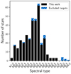 |
Fig. 1 Histogram of the M-dwarf sample analysed in this work (black) and the excluded CARMENES GTO targets (blue). |
GTO M dwarfs excluded from the analysis.
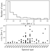 |
Fig. 2 Distribution of projected rotational velocities larger than 2 km s−1 in the sample. |
3 Analysis
In the following we describe the processing of the CARMENES observations, the selection of the spectral features to be compared with the synthetic spectra, the computation of the synthetic grid by means of the BT-Settl models and turbospectrum, and the analysis of the sample with the STEPARSYN code.
3.1 Spectral processing
All M dwarfs considered have been observed with CARMENES at several epochs since January 2016 (Reiners et al. 2018; Quirrenbach et al. 2020). The spectra were reduced following the standard CARMENES data flow. They were processed and calibrated in wavelength with the caracal pipeline (Caballero et al. 2016b). The wavelength calibration relies on a combination of hollow cathode lamps and two temperature- and pressure-stabilised Fabry-Pérot units that ensure median uncertainties of about 1 m s−1 in the VIS channel (Trifonov et al. 2018; Zechmeister et al. 2018). As an additional step in the data flow, individual spectra were corrected for telluric absorption before the co-addition into template spectra as a way to increase the S/N. The modelling of the telluric spectra was done with the software package molecfit2 (Smette et al. 2015; Kausch et al. 2015), which incorporates the line-by-line radiative transfer code LBLRTM (Clough et al. 2005)and the HITRAN molecular line list (Rothman et al. 2009). Further details on the removal of the telluric features can be found in Nagel (2019). The radial velocity pipeline serval (Zechmeister et al. 2018) co-adds all individual spectra and provides one high-S/N template spectrum per star and instrument channel. We transformed the wavelengths onto the air scale following the International Astronomical Union standard (Morton 2000) and corrected the spectra for the Doppler shift using the corresponding radial velocities of the targets.
Reference stars for the selection of Fe I and Ti I lines.
3.2 Selection of spectral features and line masks
The selection of Fe I and Ti I lines employed in this work was the result of a careful inspection of the template spectra of three representative early-, mid-, and late-type M dwarfs, namely GX And, Luyten’s star, and Teegarden’s star (see Table 2). These M dwarfs show no significant rotation or activity, except for Teegarden’s star, which shows relatively little activity for its spectral type (Zechmeister et al. 2019). In addition, their template spectra have a very high S/N. This choice of reference stars mirrors that of Reiners et al. (2018) for their spectral atlas.
For this purpose, we first requested several line lists from the Vienna Atomic Line Database3 (VALD3; Ryabchikova et al. 2015) via the extract all option, across the VIS and NIR wavelength regions covered by CARMENES. Following the prescriptions of Passegger et al. (2019), we excluded all Fe I and Ti I lines in the NIR channel (λ > 9600Å) with large Landé factors (i.e. geff > 1.5) to alleviate the impact of the stellar magnetic field on the line profiles. The visual inspection was complemented by a literature search to include some of the Fe I and Ti I line selections of Tabernero et al. (2018) and Passegger et al. (2019). The final list of 75 Fe I and Ti I lines along with the synthesised wavelength ranges can be found in Table B.2. The ranges are wide enough (i.e. a few Å) to circumvent potential problems posed by convolution at the edges. We also included the TiO γ and ϵ bands for the present analysis (see Table 3) given their high sensitivity to Teff (Rajpurohit et al. 2014; Passegger et al. 2016). In Fig. 3 we show the template spectra of the three reference stars along with the selected wavelength ranges (see also Figs. 6 and 7). In contrast to some of the lines used inother works, such as K I (Passegger et al. 2018, 2019; Rajpurohit et al. 2018b), non-LTE effects are negligible for Fe I and Ti I lines (Olander et al. 2021).
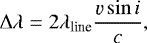
We followed Tabernero et al. (2021) to define the wavelength regions around the observed Fe I and Ti I line profiles in the template spectra to be compared with the synthetic grid (i.e. the line masks). We first performed a preliminary Gaussian fit to the Ti I and Fe I lines by means of the Levenberg-Marquardt algorithm through the Python scipy package (Virtanen et al. 2020). Next, we adjusted the line profiles assuming an initial width of 3σ around their centre, avoiding adjacent spectral features. For targets with v sin i > 4 km s−1 where the Gaussian approximation may no longer accurately reproduce the line profiles, we also broadened these line regions to account for rotation following the expression (Tabernero et al. 2021):
 (1)
(1)
where Δλ is the broadening, λline is the central wavelength of the line, and c is the speed of light.
For active stars (as indicated by the Hα flag), we specifically excluded some Fe I and Ti I lines that appear to be particularly sensitive to chromospheric activity and the stellar magnetic field. These lines are marked as magnetically sensitive in Table B.2 and will be discussed in a future publication (López-Gallifa et al., in prep.; for more details, see Montes et al. 2020). This additional consideration is particularly relevant for M dwarfs showing magnetic fields that can be as high as several kilogauss, such as EV Lac and YZ CMi (Shulyak et al. 2019). Overall, the line exclusion affected a total of 91 active stars in our sample and proved crucial in reaching convergence and, thus, avoiding getting unreliable parameters with STEPARSYN.
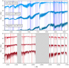 |
Fig. 3 CARMENES template spectra of GX And (M1.0 V, J00183+440), Luyten’s star (M3.5 V, J07274+052), and Teegarden’s star (M7.0 V, J02530+168) in the VIS channel (top panel) and the NIR channel (bottom panel). Blue and red shaded regions denote the ranges synthesised in this work. The two wide spectral gaps in the NIR channel shown as hatched rectangles correspond to regions severely affected by telluric absorption (Reiners et al. 2018). Inter- and intra-order gaps in the NIR channel are also shown, as grey shaded regions. |
TiO bands and wavelength ranges synthesised.
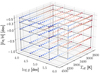 |
Fig. 4 Coverage of our synthetic grid in Teff, log g, and [Fe/H]. |
3.3 Synthetic grid
After the line selection step, we computed a coarse grid of synthetic spectra based on a set of BT-Settl model atmospheres (Allard et al. 2012)and the 1D LTE spectrum synthesis code turbospectrum (Alvarez & Plez 1998; Plez 2012). The grid is representative of the M-dwarfregime and ranges from 2600 to 4500 K and 4.0 to 6.0 dex, when available (i.e. 5.5 dex instead for models with Teff> 4000 K) in steps of 100 K and 0.5 dex in Teff and logg, respectively (see Fig. 4). We set the metallicity, [Fe/H], to the following values: −1.0, −0.5, 0.0, +0.3, and +0.5 dex. For all models, we adopted the same micro-turbulence velocities as in the PHOENIX-ACES library of synthetic spectra4 (Husser et al. 2013). We assumed the solar abundances as reported by Asplund et al. (2009) and scaled the abundances of the α elements (O, Ne, Mg, Si, S, Ar, Ca, and Ti) following the discussion of Gustafsson et al. (2008) for the standard grid of MARCS models, so that [α/Fe] = −0.4[Fe/H] for −1.0 ≤ [Fe/H] < 0.0, and [α/Fe] = 0.0 (i.e. no enhancement) for [Fe/H] ≥ 0.0. The synthetic grid was finally stored in a binary file by means of the Python module pickle (Van Rossum 2020).
The atomic data were gathered via automatic email requests to the VALD3 database using the extract all option for all the ranges listedin Tables 3 and B.2. The required molecular data were compiled from several sources and included H2O (Barber et al. 2006), FeH (Dulick et al. 2003), MgH (Kurucz 2014), CO (Goorvitch 1994), SiH (Kurucz 2014), OH (Kurucz 2014), VO (McKemmish et al. 2016), CaH, ZrO, and TiO (B. Plez, priv. comm.; see Heiter et al. 2021). To reduce computation times, we only considered the most relevant transitions in each molecular line list by applying the following Boltzmann cut (Gray 2008):
![Mathematical equation: \begin{equation*} \log{({gf\cdot\lambda_i})}-\chi_i\cdot\theta > \max_i[ \log{({gf\cdot\lambda_i})}-\chi_i\cdot\theta]-5, \end{equation*}](/articles/aa/full_html/2021/12/aa41980-21/aa41980-21-eq2.png) (2)
(2)
where λi denotes the wavelength in Å of the transition i, log gf is the oscillator strength, χi is the excitation potential in eV, and θ = 5040 K∕T, with T = 3000 K.
As discussed in Tabernero et al. (2021), the STEPARSYN code allows the synthetic grid to be sequentially convolved on the fly (i.e. prior to the comparison with the observed spectra) to account for both the stellar rotation and the instrumental profile as the main sources of spectral broadening. As for rotation, we assumed the rotational profile with a limb darkening coefficient of 0.6 from Gray (2008), and adopted the projected rotational velocities from Table B.1. Finally, to account for the instrumental profile, we convolved the spectra with a Voigt profile, assuming the corresponding median averaged Gaussian and Lorentzian components for the CARMENES VIS and NIR channels (Nagel 2019).
3.4 STEPARSYN
STEPARSYN is a Bayesian code written in Python 3 designed to map the probability distributions of the stellar atmospheric parameters (Teff, log g, [Fe/H], and vsini) from a given observed spectrum following an Markov chain Monte Carlo approach (Tabernero et al. 2021). It has already been employed in many astrophysical contexts, including the study of stars in open clusters (Lohr et al. 2018; Alonso-Santiago et al. 2019), stars in galaxies of the Local Group (Tabernero et al. 2018), and exoplanet host stars (Borsa et al. 2021; Demangeon et al. 2021).
In broad terms, the STEPARSYN code compares the observed spectrum with a grid of synthetic spectra computed around particular features. Prior decomposition of the synthetic grid following a principal component analysis (Francis & Wills 1999) helps to assess any given point of the parameter space in a computationally inexpensive way. STEPARSYN finally returns the marginalised posterior distributions in the stellar atmospheric parameters, as shown in Fig. 5 for a representative case (the M1.0 V star HD 233153), along with the best synthetic fits for the atomic lines and molecular bands, as shown in Figs. 6 and 7, respectively, for the same star (see Figs. A.1–A.9 for the reference stars GX And, Luyten’s star, and Teegarden’s star). The corner plot showing the marginalised posterior distribution obtained with STEPARSYN was made with the Python pygtc package (Bocquet & Carter 2016). Further details about STEPARSYN can be found in Tabernero et al. (2021).
To avoid degeneracies in the M-dwarf parameter space, particularly between log g and [Fe/H], we assumed Gaussian prior probability distributions in Teff and logg centred according tothe Teff, stellar mass, and radius reported by Cifuentes et al. (2020) for each target when available5, or otherwise the averaged parameters as listed in Table 6 in Cifuentes et al. (2020), with standard deviations of 200 K and 0.2 dex, respectively.Teff and logg prior distributions for our sample are included in Table B.3. These Teff values were derived from a thorough multi-band photometric analysis carried out with the Virtual Observatory Spectral energy distribution Analyser (vosa; Bayo et al. 2008), whereas the stellar radii and masses were obtained from the Stefan-Boltzmann law and the mass-radius relation derived by Schweitzer et al. (2019), respectively.
In Fig. 8 we show a Kiel diagram (i.e. log g versus Teff ) of the prior Teff and log g values that we adopted for our sample. Some stars show low logg values, which can be explained with stellar age. These stars were already identified as young stars by Schweitzer et al. (2019) on account of their membership in young stellar kinematic groups (Cortés-Contreras et al., in prep.). Among these are the Local Association, β Pictoris Moving Group, the IC 2391 Supercluster, and Castor Moving Group, with estimated ages of 10–150 Ma (Bell et al. 2015), 18.5 Ma (Miret-Roig et al. 2020), 50 Ma (Barrado y Navascués et al. 2004), and 440 Ma (Mamajek et al. 2013), respectively. On the contrary, a few additional targets exhibit a high log g, probably due to their behaviour akin to subdwarfs, following the discussion by Schweitzer et al. (2019). All these outliers in log g are listed in Table 4.
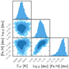 |
Fig. 5 Marginalised posterior distributions in Teff, log g, and [Fe/H] for the M1.0 V star HD 233153 (J05415+534). The colour shades denote the 1σ, 2σ, and 3σ levels. The retrieved parameters are Teff = 3825 ± 14 K, log g =4.94 ± 0.10 dex, and [Fe/H] = −0.04 ± 0.06 dex. |
4 Results and discussion
The stellar atmospheric parameters of the sample computed with STEPARSYN (Teff, log g, [Fe/H]) are given in Table B.3. Since some M-dwarf studies do not consider alpha enhancement in the computation of synthetic spectra (see e.g. Passegger et al. 2018), we corrected our [Fe/H] scale into [Fe/H]corr in order to compare our results more directly with that of the literature. We did this through a linear interpolation scheme via the scipy package between the mass fraction of elements heavier than helium (Z) and the corresponding [Fe/H] valuein alpha-enhanced and alpha-solar (i.e. no alpha enhancement) models, respectively, as shown in Fig. 9. The correspondence between Z and [Fe/H] was adopted from the MARCS atmosphere models with standard and alpha-poor compositions6. The interpolation scheme retrieves the [Fe/H]corr value that corresponds to a given Z defined by the original [Fe/H] scale.
We note the limitations of our methodology with respect to the analysis of M dwarfs with spectral types M8.0 V or later due to the scarcity of useful Fe I and Ti I lines and the poor sensitivity of the TiO molecular bands to Teff as a result of dust formation in the stellar photospheres (Tsuji et al. 1996; Allard et al. 2001). Furthermore, the version of the BT-Settl models used in this work does not allow for the formation of enough dust in very late M dwarfs (Allard et al. 2012). However, wenote that this limit in spectral type is similar to other studies based on spectral synthesis in M dwarfs (Rajpurohit et al. 2018b; Schweitzer et al. 2019).
We compared our results against some recent M-dwarf studies, including Passegger et al. (2019, Fig. 10), Rojas-Ayala et al. (2012, Fig. A.10), Gaidos & Mann (2014, Fig. A.11), Maldonado et al. (2015, Fig. A.12), Mann et al. (2015, Fig. A.13), Passegger et al. (2018, Fig. A.14), Rajpurohit et al. (2018b, Fig. A.15), Schweitzer et al. (2019, Fig. A.16), Maldonado et al. (2020, Fig. A.17), and Passegger et al. (2020, Fig. A.18). The approaches to the computation of stellar parameters in the M-dwarf regime are manifold and generally dependent on the covered wavelength region Δλ, the spectral resolution R, and the S/N of the spectra. For instance, Teff can be derived from the H2O-K2 index (Rojas-Ayala et al. 2012), the pseudo-EW of spectral features (Maldonado et al. 2015, 2020), and spectral fitting to a variety of synthetic grids, including PHOENIX-ACES (Passegger et al. 2018; Schweitzer et al. 2019), PHOENIX-SESAM (Passegger et al. 2019), and grids based on BT-Settl models (Gaidos & Mann 2014; Mann et al. 2015; Rajpurohit et al. 2018b). As for log g, in some studies it is left as a free parameter in the fitting procedure (Rajpurohit et al. 2018b), while in others log g is kept fixed instead based on evolutionary models to break the observed degeneracy in the M-dwarf parameter space (Rojas-Ayala et al. 2012; Passegger et al. 2018, 2019). In other cases, log g is derived indirectly from the stellar masses and radii obtained from different approaches, primarily semi-empirical calibrations (Gaidos & Mann 2014; Mann et al. 2015; Maldonado et al. 2015, 2020; Schweitzer et al. 2019). Lastly, stellar metallicity is usually derived from semi-empirically calibrated relations established between the spectral features of M dwarfs that are companions of FGK-type stars with known metallicities (Terrien et al. 2012; Mann et al. 2013a, 2014, 2015; Newton et al. 2014; Neves et al. 2014; Maldonado et al. 2015, 2020), and the use of weights in the spectral fitting for spectral features that appear to be more sensitive to metallicity variations (Passegger et al. 2016, 2018, 2019).
To explore possible sources of systematic trends or offsets, we followed the same Monte Carlo method as in Tabernero et al. (2018). We generated 10 000 artificial samples based on the stellar atmospheric parameters derived with STEPARSYN by assuming a normal distribution centred at the original measurements, and widths equal to the uncertainties in the parameters. The summary of these Monte Carlo simulations can be found in Table 5. We computed the Pearson (rp ) and the Spearman (rs) correlation coefficients, which quantify the degree of correlation between any two given variables. Our temperature scale appears to have an intrinsic systematic offset relative to the literature values in the range from 4 to 85 K. The offset is smallest for Gaidos & Mann (2014) and largest for Mann et al. (2015). In other words, all literature sources report on average slightly lower effective temperatures. However, we note that the offsets are compatible with zero in all instances but Mann et al. (2015). Regarding log g, our values appear to be higher (between 0.02 and 0.17 dex on average with respect to the literature), except for Rajpurohit et al. (2018b), although even in that case the discrepancies are compatible with zero. As to metallicity, our [Fe/H] scale seems to agree best with the results by Rojas-Ayala et al. (2012), Mann et al. (2015), and Maldonado et al. (2015, 2020). In contrast, large discrepancies in metallicity can be seen when comparing our results with Passegger et al. (2018, 2019), and Schweitzer et al. (2019). Among the plausible explanations are the use of different synthetic models, minimisation algorithms, and sets of lines in their analyses, especially K I lines, which have been shown to be affected by non-LTE effects that can translate into metallicity corrections of the order of 0.2 dex (Olander et al. 2021).
Regarding the comparison between our results and the prior distributions, we find that the spectroscopic Teff values are higher by 136 ± 88 K, which is in agreement with the findings of Cifuentes et al. (2020) when comparing their estimations using photometry and vosa to spectroscopic studies, namely Passegger et al. (2019) and Rajpurohit et al. (2018b). This difference is in turn more noticeable towards the mid-type and late M dwarfs, probably due to missing opacity sources. Regarding log g, it also seems to be higher by0.08 ± 0.14 dex with respectto the prior values.
Similarly to Figs. 8, 11 is a Kiel diagram of our sample showing the results obtained with STEPARSYN along with theoretical isochrones from the PAdova and TRieste Stellar Evolution Code (PARSEC; Bressan et al. 2012). Since M dwarfs evolve very slowly once they reach the main sequence (Burrows et al. 1997), we selected a set of isochrones with an age of 5 Ga and different compositions, namely [Fe/H] = −0.4, 0.0, and 0.2 dex. Active and inactive stars in Fig. 11 are shown with different symbols. First, we note that the fraction of active stars increases towards the late M-dwarf regime, as discussed by Tal-Or et al. (2018) and Reiners et al. (2018). While some stars fall inside the region encompassed by the isochrones, we note that most of them deviate towards higher values of log g. However, the trend established by the isochrones is preserved in the retrieved log g values throughout the diagram. Additionally, conspicuous outliers have been labelled and marked with red and blue circles. Red circles denote seven of the ten targets identified as young according to Table 4, whereas blue circles indicate other stars that also correspond to higher logg values. We note that most of them are active stars, with the exception of the early M dwarfs BD+21 652 and HD 275122.
In light of such a large dispersion in logg, we performed an additional run by fixing logg to the prior values. The results of this run (Teff, fixed, [Fe/H]fixed, and [Fe/H]corr, fixed) can also be found in Table B.3. In Fig. 12 we show the differences in Teff and [Fe/H] between these two runs. The impact of fixing logg on Teff is well below 100 K for most targets, whereas the impact on [Fe/H] is between 0.1 and 0.2 dex in most cases. In general terms, the larger the difference in logg between the runs, the larger the change in [Fe/H], as expected.
To check our metallicity scale, in Fig. 13 we compare the M-dwarf metallicity distribution presented in this work to that from the Geneva-Copenhagen survey (Nordström et al. 2004), which comprises around 14 000 F- and G-type dwarfs in the solar neighbourhood, and is volume-complete to a distance of ~40 pc. We note that the two distributions are very similar in the low-metallicity regime, whereas high-metallicity stars appear to be marginally underrepresented. There appears to be an excess of M dwarfs with solar metallicity and we retrieve no metallicity higher than 0.25 dex. The scarcity of high-metallicity values is also noticeable when comparing our determinations with the literature, as shown in Figs. A.10 (Rojas-Ayala et al. 2012), A.11 (Gaidos & Mann 2014), and Fig. A.13 (Mann et al. 2015).
We also investigated the M-dwarf metallicity distribution in terms of the kinematic membership of the stars in the Galactic populations, namely the thick disc (TD), the thick disc-thin disc transition (TD-D), the thin disc (D), and the young disc (YD) (Montes et al. 2001; Cortés-Contreras et al., in prep.), as shown in Fig. 14. It can be seen that the mean metallicity of M dwarfs belonging to the TD is lower than that of those belonging to the D, in accordance with the results presented by Bensby et al. (2003, 2005).
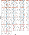 |
Fig. 6 Atomic line fits for the M1.0 V star HD 233153 (J05415+534). The solid black and orange lines are the observed and synthetic spectra, respectively. The blue and pink shaded areas are the regions of comparison between the observed and the synthetic spectra (i.e. line masks) forfeatures in the VIS and NIR channels of CARMENES, respectively. The vertical dashed black lines mark the central wavelengths. The species, the central wavelength, and the effective Landé factor, geff, of the lines are indicated inside each box. |
Outliers in log g.
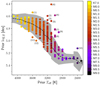 |
Fig. 8 Central prior Teff and log g values for the sample following Cifuentes et al. (2020). The spectral types are colour-coded. The dashed black line is the average Teff and log g for K7 V to M9.0 V objects, with the corresponding uncertainties shaded in grey. The 15 outliers discussed in Sect. 3.4 are labelled and listed in Table 4. Two and three stars are superimposed under labels (7) and (11), respectively. |
Summary of the Monte Carlo simulations on Teff, log g, and [Fe/H] between different comparison samples.
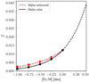 |
Fig. 9 Interpolation scheme between Z and [Fe/H] in alpha-enhanced (red) and alpha-solar (black) models. |
4.1 M dwarfs with interferometric angular measurements
In Table 6 we compile the 18 M dwarfs in our sample with interferometrically measured radii from Boyajian et al. (2012) and von Braun et al. (2014), which may be used along with other information (e.g. trigonometric parallax, bolometric flux, isochrone fitting, and mass-luminosity relations) to derive Teff and log g independently from spectroscopy. For this reason, this set of stars is particularly helpful as a benchmark test for any method aimed at determining stellar atmospheric parameters (Casagrande et al. 2008; Mann et al. 2015; Birky et al. 2020).
Figure 15 shows the comparison in Teff and logg for these M dwarfs between Boyajian et al. (2012), von Braun et al. (2014), and this work. The log g value was computed from the stellar mass and radius using the standard definition (i.e. g = GM∕R2, where G is the gravitational constant). In general, we find good agreement, with systematic offsets of 72 ± 67 K in Teff, and 0.10± 0.09 dex in log g. However, we note two outliers in Teff, namely Il Aqr and HD 173740, which show a difference around 300 K between the interferometric and the spectroscopic approaches. Interestingly enough, HD 173740 also belongs to a wide binary system together with HD 173739, as discussed in Sect. 4.3. Although they exhibit similar chemical compositions and differ by only one spectral subtype, the Teff derived from interferometry appears to be irreconcilable between the two components. In contrast, we derived very similar Teff with STEPARSYN for both components. However, accounting for this difference is beyond the scope of this paper.
4.2 M dwarfs in FGK+M systems
The study of multi-star systems serves as a benchmark test for [Fe/H] given that all components are thought to be formed from the same molecular cloud, be coeval, and have roughly similar chemical compositions (Desidera et al. 2006; Önehag et al. 2012; Souto et al. 2020; Ishikawa et al. 2020). In Table 7 we compile all M dwarfs in our sample that are bound in wide physical binaries with an FGK-type primary (Montes et al. 2018). For the FGK-type primaries, we adopted the metallicities from Montes et al. (2018), who employed the STEPAR code (Tabernero et al. 2019) as the preferred implementation of the EW method. For the fast-rotating F7 V star θ Boo A (v sini = 30.4 km s−1, Luck 2017), we adopted the metallicity from Tabernero et al. (2021).
In Fig. 16 we show the comparison in [Fe/H] between the components in these FGK+M systems. We find good agreement between our [Fe/H] determinations for the M-dwarf secondaries, with an internal scatter of − 0.01 ± 0.19 dex, which is similar to what is found in other works (Souto et al. 2020; Antoniadis-Karnavas et al. 2020). The largest discrepancy in metallicity between components is found for ρ Cnc B. If we assume a homogeneous chemical composition in FGK+M systems, this star also exhibits a C/O ratio that is larger than expected for an M dwarf, since C/O = 1.12 for the primary star (Delgado Mena et al. 2010). We note that the pseudo-continuum level is very sensitive to C/O and alterations in C/O can explain a large fraction of the variation in the strength of the atomic metal lines in M-dwarf spectra (Veyette et al. 2016; Souto et al. 2020). However, disentangling the effect of C/O on [Fe/H] computations is beyond the scope of this paper.
4.3 M dwarfs in M+M systems
Similarly to FGK+M systems, wide physical M+M binaries can also prove useful as a benchmark test for [Fe/H]. In this case, both components are analysedwith the same methodology (i.e. spectral synthesis). In Table 9 we list the astrometric parameters (parallax π, proper motion μ, and radial velocity vr ) along with the stellar atmospheric parameters (Teff, log g, and [Fe/H]) of the 32 M dwarfs in our sample bound in M+M systems. These include two SB2 systems (EZ Psc and GJ 810) and the M8.0 V star V1298 Aql (vB 10), for which no reliable parameter determinations could be made (see Table 1). Parallaxes and proper motions were compiled from the Gaia DR2 and EDR3 releases (Gaia Collaboration 2018, 2021).
In Fig. 16 we compare the metallicity computed in this work for both components, in the same way as for the FGK+M wide binaries. The mean difference in [Fe/H] between components is 0.10 ± 0.08 dex, which is in agreement with other works (0.06 ± 0.07 dex, Antoniadis-Karnavas et al. 2020). However, we note that the differences become larger (i.e. up to ~0.2 dex) in cases where the components differ by more than one spectral type.
4.4 Choice of model atmospheres
Recent studies have shown that different parameter determination methods can lead to significant variations in the results for the same stars (Blanco-Cuaresma 2019; Passegger et al. 2021). These differences can be attributed to a number of factors, including the choice of model atmospheres, atomic and molecular data, and radiative transfer code. For this reason, we performed a test on the reference stars (i.e. GX And, Luyten’s star, and Teegarden’s star) with the aim of evaluating the impact of different sets of models on our parameter computations with STEPARSYN.
We first computed a synthetic grid based on MARCS models by following the same procedure as described in Sect. 3.3. We set the MARCS grid from 2500 to 3900 K, 4.0 to 5.5 dex, and −1.0 to +1.0 dex, in steps of 100 K, 0.5 dex, and 0.25 dex in Teff, log g, and [Fe/H], respectively.Similarly, we adopted the PHOENIX-ACES grid used by Passegger et al. (2021), which ranges from 2700 to 4500 K, 4.2 to 5.5 dex, and −1.0 to +0.8 dex, in steps of 100 K, 0.1 dex, and 0.1 dex in Teff, log g, and [Fe/H], respectively. While the MARCS grid is based on atmosphere models with standard composition and, thus, follows the same scaled [α∕Fe] pattern as the BT-Settl grid, the PHOENIX-ACES grid has [α∕Fe] = 0 since modelswith [α∕Fe]≠0 are only available for Teff > 3500 K (Husser et al. 2013; Passegger et al. 2018). Therefore, metallicities derived with the PHOENIX-ACES grid do not need to be corrected with the interpolation scheme described in Sect. 4.
In Table 8 we list the parameters obtained for the reference stars and the considered grids (i.e. BT-Settl, MARCS, and PHOENIX-ACES). The derived log g and [Fe/H] values agree within the uncertainties for all models, while the average differences in Teff, log g, and [Fe/H] between models are around 32 K, 0.11 dex, and 0.06 dex, respectively. In addition, the derived Teff values appear to be slightly higher when using MARCS and PHOENIX-ACES models. In contrast, log g values are slightly lower. The differences in these results might arise from the synthetic gap (Passegger et al. 2020), that is, the fact that synthetic spectra do not perfectly match the observed spectra as a result of the underlying chemo-physical assumptions (e.g. different equations of state). However, a more detailed study is required to further explore the origin of these small discrepancies.
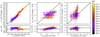 |
Fig. 10 Comparison between this work and the VIS+NIR analysis done by Passegger et al. (2019). Spectral types are colour-coded. The dashed black lines indicate the 1:1 relationship. |
Mdwarfs with interferometric angular diameter measurements in common with the CARMENES GTO survey.
Mdwarfs in wide physical binaries with FGK-type primaries in common with the CARMENES GTO survey.
Parameters derived for the reference stars with different synthetic grids.
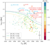 |
Fig. 11 Kiel diagram of the sample showing the parameters computed with STEPARSYN. Squares depict Hα-active stars. The metallicity [Fe/H]corr is colour-coded. Lines correspond to 5-Ga PARSEC isochrones with [Fe/H] = −0.4, 0.0, and 0.2 dex (Bressan et al. 2012). Typical uncertainties in logg and Teff are shown in the bottom-right corner. Outliers in logg are marked with red and blue circles (see Sect. 4 for details). |
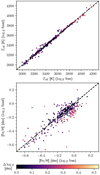 |
Fig. 12 Comparison of Teff (top panel) and [Fe/H] (bottom panel) between the runs with free and fixed log g. The quantity Δlogg is calculated as logg (prior) − logg (free). |
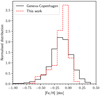 |
Fig. 13 Metallicity distribution in this work and in the Geneva-Copenhagen survey (Nordström et al. 2004). |
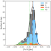 |
Fig. 14 M-dwarf metallicity distributions separated by the kinematic membership of the targets in the thick disc (TD), the thick disc-thin disc transition (TD-D), the thin disc (D), and the young disc (YD), following Cortés-Contreras et al. (in prep.). The vertical dashed lines indicate the peak of the distributions. |
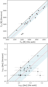 |
Fig. 15 Comparison in Teff (upper panel) and logg (bottom panel) for M dwarfs with interferometric angular measurements (see Table 6). The dashed black lines indicate the 1:1 relationship, whereas the dotted red lines show the 1:1 relationship, shifted following the average differences in each parameter. The blue shaded region denotes the 1σ level. |
5 Summary and conclusions
We have computed the stellar atmospheric parameters (Teff, log g, [Fe/H], and [Fe/H]corr) of 343 M dwarfs observed with CARMENES with the STEPARSYN code as a Bayesian implementation of the spectral synthesis technique, along with a grid of BT-Settl models, and the radiative transfer code turbospectrum. We excluded one eclipsing binary, ten SB2 binaries, two triple-line spectroscopic triple systems, and three targets with low-quality spectra to prevent unreliable parameter determinations. To avoid any potential degeneracy in the M-dwarf parameter space, we imposed prior probability distributions in Teff and log g based on the comprehensive, multi-band photometric data available for the sample (Cifuentes et al. 2020). Our method is suited for the M sequence from M0.0 V to M7.0 V, but not beyond, due to the scarcity of Ti I and Fe I lines at M8.0 V and later spectral types, as well as the insensitivity of TiO bands to Teff as a result of dust formation (Tsuji et al. 1996; Allard et al. 2001).
We selected 75 Fe I and Ti I lines in the VIS and NIR wavelength regions covered by CARMENES. Following the prescriptions of Passegger et al. (2019), NIR lines with low Landé factors (i.e. geff < 1.5) were selected to minimise the impact of the stellar magnetic field on parameter computations. Even so, some Fe I and Ti I lines appear to be highly sensitive to chromospheric activity and the stellar magnetic field and were excluded in the analysis of the active stars in our sample based on the Hα flag. Such lines will be discussed in a future publication (López-Gallifa et al., in prep.).
We also compared our derived parameters with some recent M-dwarf studies in the literature (Rojas-Ayala et al. 2012; Maldonado et al. 2015, 2020; Mann et al. 2015; Rajpurohit et al. 2018b; Schweitzer et al. 2019; Passegger et al. 2018, 2019, 2020), finding similar Teff but disparate metallicity scales. The metallicity determinations that correlate best with the literature are the [Fe/H]corr values since they are corrected from the α enhancement of the synthetic grid. The best agreement in metallicity is found when comparing with Mann et al. (2015), Gaidos & Mann (2014), and Rojas-Ayala et al. (2012). The M-dwarf metallicity distribution for our sample is also in agreement with both the Geneva-Copenhagen survey of FG-type stars in the solar neighbourhood (Nordström et al. 2004) and the kinematic membership of the targets in the Galactic populations (Cortés-Contreras et al., in prep.). Regarding log g, we find larger values than the ones reported in the literature, although fixing log g to the prior values does not have a strong impact on either the derived Teff or the [Fe/H] scales. As a benchmark test, we placed special emphasis on the M dwarfs with interferometrically measured radii (Boyajian et al. 2012; von Braun et al. 2014), wide physical FGK+M binaries (Montes et al. 2018), and M+M systems. Despite systematic offsets that are inherent to any methodology, we find that our parameter determinations are fairly consistent with the literature values in all these cases.
Astrometric and stellar atmospheric parameters of the M dwarfs bound in M+M systems in the CARMENES GTO sample.
 |
Fig. 16 Same as Fig. 15, but for the comparison in [Fe/H] between the components in FGK+M (blue) and M+M (red) systems (see Tables 7 and 9). |
Acknowledgements
We thank the anonymous referee for the insightful comments and suggestions that improved the manuscript of the paper. CARMENES is an instrument for the Centro Astronómico Hispano en Andalucía at Calar Alto (CAHA). CARMENES is funded by the German Max-Plank Gesellschaft (MPG), the Spanish Consejo Superior de Investigaciones Científicas (CSIC), the European Union through FEDER/ERF FICTS-2011-02 funds, and the members of the CARMENES Consortium (Max-Plank-Institut für Astronomie, Instituto de Astrofísica de Andalucía, Landessternwarte Königstuhl, Institut de Ciènces de l’Espai, Institut für Astrophysik Göttingen, Universidad Complutense de Madrid, Thüringer Landessternwarte Tautenberg, Instituto de Astrofísica de Canarias, Hamburger Sternwarte, Centro de Astrobiología and Centro Astronómico Hispano-Andaluz), with additional contributions by the Spanish Ministry of Economy, the German Science Foundation through the Major Research Instrumentation Programme and DFG Research Unit FOR2544 “Blue Planets around Red Stars”, the Klaus Tschira Stiftung, the states of Baden-Württemberg and Niedersachsen, and by the Junta de Andalucía. The authors acknowledge financial support from the Fundação para a Ciência e a Tecnologia (FCT) through the research grants UID/FIS/04434/2019, UIDB/04434/2020 and UIDP/04434/2020, national funds PTDC/FIS-AST/28953/2017, by FEDER (Fundo Europeu de Desenvolvimento Regional) through COMPETE2020 – Programa Operacional Competitividade e Internacionalização (POCI-01-0145-FEDER-028953), and the Spanish Ministerio de Ciencia, Innovación y Universidades, Ministerio de Economía y Competitividad, the Universidad Complutense de Madrid, and the Fondo Europeo de Desarrollo Regional (FEDER/ERF) through fellowship FPU15/01476, and projects AYA2016-79425-C3-1/2/3-P, PID2019-109522GB-C5[1:4]/AEI/10.13039/501100011033, AYA2014-56359-P, BES-2017-080769, and RYC-2013-14875. The authors also acknowledge financial support from the Centre of Excellence “Severo Ochoa” and “María de Maeztu” awards to the Instituto de Astrofísica de Canarias (SEV-2015-0548), Instituto de Astrofísica de Andalucía (SEV-2017-0709), and Centro de Astrobiología (MDM-2017-0737), and the Generalitat de Catalunya/CERCA programme. This work has made use of the VALD database, operated at Uppsala University, the Institute of Astronomy RAS in Moscow, and the University of Vienna, and of data from the European Space Agency (ESA) mission Gaia (https://www.cosmos.esa.int/gaia), processed by the Gaia Data Processing and Analysis Consortium (DPAC, https://www.cosmos.esa.int/web/gaia/dpac/consortium). Funding for the DPAC has been provided by national institutions, in particular the institutions participating in the Gaia Multilateral Agreement. V.M.P. acknowledges financial support from NASA through grant NNX17AG24G. S.V.J. acknowledges the support of the DFG priority program SPP 1992 “Exploring the Diversity of Extrasolar Planets” (JE 701/5-1). E.M. would also like to warmly thank the staff at the Hamburger Sternwarte for their hospitality during his stay funded by project EST18/00162. Based on data from the CARMENES data archive at CAB (INTA-CSIC).
Appendix A Additional figures
Figures A.1, A.2, and A.3 show the marginalised posterior distributions in Teff, log g, and [Fe/H] for the reference stars, namely GX And, Luyten’s star, and Teegarden’s star, respectively (see Table 2). The best synthetic fits for the atomic lines and molecular bands for these stars can be found in Figs. A.4, A.5, A.6, A.7, A.8, and A.9.
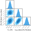 |
Fig. A.1 Same as Fig. 5, but for GX And (M1.0 V, J00183+440). The retrieved parameters are Teff = 3603 ± 24 K, log g =4.99 ± 0.14 dex, and [Fe/H] = −0.75 ± 0.11 dex. |
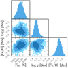 |
Fig. A.2 Same as Fig. 5, but for Luyten’s star (M3.5 V, J07274+052). The retrieved parameters are Teff = 3380 ± 43 K, log g =4.96 ± 0.11 dex, and [Fe/H] = −0.17 ± 0.11 dex. |
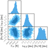 |
Fig. A.3 Same as Fig. 5, but for Teegarden’s star (M7.0 V, J02530+168). The retrieved parameters are Teff = 3034 ± 45 K, log g =5.19 ± 0.20 dex, and [Fe/H] = −0.17 ± 0.28 dex. |
Figures A.10, A.11, A.12, A.13, A.14, A.15, A.16, A.17, and A.18 show the comparison between our results and those of Rojas-Ayala et al. (2012), Gaidos & Mann (2014), Maldonado et al. (2015), Mann et al. (2015), Passegger et al. (2018), Rajpurohit et al. (2018a), Schweitzer et al. (2019), Maldonado et al. (2020), and Passegger et al. (2020), respectively, as discussed in Sect. 4.
 |
Fig. A.10 Comparison between this work and Rojas-Ayala et al. (2012). |
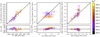 |
Fig. A.11 Comparison between this work and Gaidos & Mann (2014). |
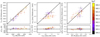 |
Fig. A.12 Comparison between this work and Maldonado et al. (2015). |
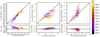 |
Fig. A.13 Comparison between this work and Mann et al. (2015). |
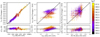 |
Fig. A.14 Comparison between this work and Passegger et al. (2018). |
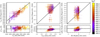 |
Fig. A.15 Comparison between this work and Rajpurohit et al. (2018a). |
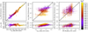 |
Fig. A.16 Comparison between this work and Schweitzer et al. (2019). |
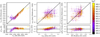 |
Fig. A.17 Comparison between this work and Maldonado et al. (2020). |
 |
Fig. A.18 Comparison between this work and Passegger et al. (2020). |
Appendix B Additional tables
Tables B.1, B.2, and B.3 are available in their entirety in a machine-readable form at the CDS. An excerpt is shown here for guidanceregarding their form and content.
Sample of M dwarfs from the CARMENES radial velocity survey analysed in this work.
Selection of Ti I and Fe I lines in the spectra of GX And (M1.0 V), Luyten’s star (M3.5 V), and Teegarden’s star (M7.0 V).
Prior Teff and log g distributions and stellar atmospheric parameters of the sample computed with STEPARSYN.
References
- Abia, C., Tabernero, H. M., Korotin, S. A., et al. 2020, A&A, 642, A227 [NASA ADS] [CrossRef] [EDP Sciences] [Google Scholar]
- Allard, F., Hauschildt, P. H., Alexander, D. R., Tamanai, A., & Schweitzer, A. 2001, ApJ, 556, 357 [Google Scholar]
- Allard, F., Homeier, D., & Freytag, B. 2012, Phil. Trans. R. Soc. London Ser. A, 370, 2765 [Google Scholar]
- Alonso-Floriano, F. J., Morales, J. C., Caballero, J. A., et al. 2015, A&A, 577, A128 [NASA ADS] [CrossRef] [EDP Sciences] [Google Scholar]
- Alonso-Floriano, F. J., Sánchez-López, A., Snellen, I. A. G., et al. 2019, A&A, 621, A74 [NASA ADS] [CrossRef] [EDP Sciences] [Google Scholar]
- Alonso-Santiago, J., Negueruela, I., Marco, A., et al. 2019, A&A, 631, A124 [NASA ADS] [CrossRef] [EDP Sciences] [Google Scholar]
- Alvarez, R., & Plez, B. 1998, A&A, 330, 1109 [NASA ADS] [Google Scholar]
- Antoniadis-Karnavas, A., Sousa, S. G., Delgado-Mena, E., et al. 2020, A&A, 636, A9 [NASA ADS] [CrossRef] [EDP Sciences] [Google Scholar]
- Asplund, M., Grevesse, N., Sauval, A. J., & Scott, P. 2009, ARA&A, 47, 481 [NASA ADS] [CrossRef] [Google Scholar]
- Baraffe, I., Chabrier, G., Allard, F., & Hauschildt, P. H. 1998, A&A, 337, 403 [Google Scholar]
- Barber, R. J., Tennyson, J., Harris, G. J., & Tolchenov, R. N. 2006, MNRAS, 368, 1087 [Google Scholar]
- Baroch, D., Morales, J. C., Ribas, I., et al. 2018, A&A, 619, A32 [NASA ADS] [CrossRef] [EDP Sciences] [Google Scholar]
- Baroch, D., Morales, J. C., Ribas, I., et al. 2021, A&A, 653, A49 [NASA ADS] [CrossRef] [EDP Sciences] [Google Scholar]
- Barrado Y Navascués, D., Stauffer, J. R., & Jayawardhana, R. 2004, ApJ, 614, 386 [CrossRef] [Google Scholar]
- Bayo, A., Rodrigo, C., Barrado Y Navascués, D., et al. 2008, A&A, 492, 277 [NASA ADS] [CrossRef] [EDP Sciences] [Google Scholar]
- Bell, C. P. M., Mamajek, E. E., & Naylor, T. 2015, MNRAS, 454, 593 [Google Scholar]
- Bensby, T., Feltzing, S., & Lundström, I. 2003, A&A, 410, 527 [CrossRef] [EDP Sciences] [Google Scholar]
- Bensby, T., Feltzing, S., Lundström, I., & Ilyin, I. 2005, A&A, 433, 185 [NASA ADS] [CrossRef] [EDP Sciences] [Google Scholar]
- Bergemann, M., Collet, R., Schönrich, R., et al. 2017, ApJ, 847, 16 [Google Scholar]
- Birky, J., Hogg, D. W., Mann, A. W., & Burgasser, A. 2020, ApJ, 892, 31 [Google Scholar]
- Blanco-Cuaresma, S. 2019, MNRAS, 486, 2075 [Google Scholar]
- Blanco-Cuaresma, S., Soubiran, C., Heiter, U., & Jofré, P. 2014, Astrophysics Source Code Library [record ascl:1409.006] [Google Scholar]
- Bochanski, J. J., Munn, J. A., Hawley, S. L., et al. 2007, AJ, 134, 2418 [Google Scholar]
- Bocquet, S., & Carter, F. W. 2016, J. Open Source Softw., 1, 1 [Google Scholar]
- Bonfils, X., Delfosse, X., Udry, S., et al. 2013, A&A, 549, A109 [NASA ADS] [CrossRef] [EDP Sciences] [Google Scholar]
- Borsa, F., Allart, R., Casasayas-Barris, N., et al. 2021, A&A, 645, A24 [EDP Sciences] [Google Scholar]
- Boyajian, T. S., von Braun, K., van Belle, G., et al. 2012, ApJ, 757, 112 [Google Scholar]
- Bressan, A., Marigo, P., Girardi, L., et al. 2012, MNRAS, 427, 127 [NASA ADS] [CrossRef] [Google Scholar]
- Brewer, J. M., Fischer, D. A., Valenti, J. A., & Piskunov, N. 2016, ApJS, 225, 32 [Google Scholar]
- Buchhave, L. A., Latham, D. W., Johansen, A., et al. 2012, Nature, 486, 375 [NASA ADS] [Google Scholar]
- Burrows, A., Marley, M., Hubbard, W. B., et al. 1997, ApJ, 491, 856 [Google Scholar]
- Caballero, J. A., Cortés-Contreras, M., Alonso-Floriano, F. J., et al. 2016a, in 19th Cambridge Workshop on Cool Stars, Stellar Systems, and the Sun (CS19) (Berlin: Springer), 148 [Google Scholar]
- Caballero, J. A., Guàrdia, J., López del Fresno, M., et al. 2016b, SPIE Conf. Ser., 9910, 99100E [Google Scholar]
- Casagrande, L., Flynn, C., & Bessell, M. 2008, MNRAS, 389, 585 [Google Scholar]
- Cifuentes, C., Caballero, J. A., Cortés-Contreras, M., et al. 2020, A&A, 642, A115 [NASA ADS] [CrossRef] [EDP Sciences] [Google Scholar]
- Claudi, R., Benatti, S., Carleo, I., et al. 2018, SPIE Conf. Ser., 10702, 107020Z [NASA ADS] [Google Scholar]
- Clough, S. A., Shephard, M. W., Mlawer, E. J., et al. 2005, J. Quant. Spectr. Rad. Transf., 91, 233 [NASA ADS] [CrossRef] [Google Scholar]
- Delfosse, X., Forveille, T., Perrier, C., & Mayor, M. 1998, A&A, 331, 581 [NASA ADS] [Google Scholar]
- Delgado Mena, E., Israelian, G., González Hernández, J. I., et al. 2010, ApJ, 725, 2349 [NASA ADS] [CrossRef] [Google Scholar]
- Demangeon, O. D. S., Zapatero Osorio, M. R., Alibert, Y., et al. 2021, A&A, 653, A41 [NASA ADS] [CrossRef] [EDP Sciences] [Google Scholar]
- Desidera, S., Gratton, R. G., Lucatello, S., & Claudi, R. U. 2006, A&A, 454, 581 [NASA ADS] [CrossRef] [EDP Sciences] [Google Scholar]
- Donati, J. F., Morin, J., Petit, P., et al. 2008, MNRAS, 390, 545 [Google Scholar]
- Donati, J. F., Kouach, D., Moutou, C., et al. 2020, MNRAS, 498, 5684 [Google Scholar]
- Dressing, C. D., & Charbonneau, D. 2013, ApJ, 767, 95 [Google Scholar]
- Dulick, M., Bauschlicher, C. W., J., Burrows, A., et al. 2003, ApJ, 594, 651 [NASA ADS] [CrossRef] [Google Scholar]
- Francis, P. J., & Wills, B. J. 1999, ASP Conf. Ser., 162, 363 [Google Scholar]
- Fuhrmeister, B., Czesla, S., Schmitt, J. H. M. M., et al. 2018, A&A, 615, A14 [NASA ADS] [CrossRef] [EDP Sciences] [Google Scholar]
- Fuhrmeister, B., Czesla, S., Hildebrandt, L., et al. 2020, A&A, 640, A52 [NASA ADS] [CrossRef] [EDP Sciences] [Google Scholar]
- Gaia Collaboration (Brown, A. G. A., et al.) 2018, A&A, 616, A1 [NASA ADS] [CrossRef] [EDP Sciences] [Google Scholar]
- Gaia Collaboration (Brown, A. G. A., et al.) 2021, A&A, 649, A1 [NASA ADS] [CrossRef] [EDP Sciences] [Google Scholar]
- Gaidos, E., & Mann, A. W. 2014, ApJ, 791, 54 [Google Scholar]
- García Pérez, A. E., Allende Prieto, C., Holtzman, J. A., et al. 2016, AJ, 151, 144 [Google Scholar]
- Goorvitch, D. 1994, ApJS, 95, 535 [NASA ADS] [CrossRef] [Google Scholar]
- Gray, D. F. 2008, The Observation and Analysis of Stellar Photospheres (Cambridge: Cambridge University Press) [Google Scholar]
- Gustafsson, B., Edvardsson, B., Eriksson, K., et al. 2008, A&A, 486, 951 [NASA ADS] [CrossRef] [EDP Sciences] [Google Scholar]
- Heiter, U., Lind, K., Bergemann, M., et al. 2021, A&A, 645, A106 [EDP Sciences] [Google Scholar]
- Hejazi, N., Lépine, S., Homeier, D., Rich, R. M., & Shara, M. M. 2020, AJ, 159, 30 [NASA ADS] [CrossRef] [Google Scholar]
- Henry, T. J., Jao, W.-C., Winters, J. G., et al. 2018, AJ, 155, 265 [NASA ADS] [CrossRef] [Google Scholar]
- Hintz, D., Fuhrmeister, B., Czesla, S., et al. 2019, A&A, 623, A136 [NASA ADS] [CrossRef] [EDP Sciences] [Google Scholar]
- Hintz, D., Fuhrmeister, B., Czesla, S., et al. 2020, A&A, 638, A115 [NASA ADS] [CrossRef] [EDP Sciences] [Google Scholar]
- Howard, A. W., Marcy, G. W., Bryson, S. T., et al. 2012, ApJS, 201, 15 [Google Scholar]
- Husser, T.-O., Wende-von Berg, S., Dreizler, S., et al. 2013, A&A, 553, A6 [NASA ADS] [CrossRef] [EDP Sciences] [Google Scholar]
- Ishikawa, H. T., Aoki, W., Kotani, T., et al. 2020, PASJ, 72, 102 [CrossRef] [Google Scholar]
- Johnson, J. A., Aller, K. M., Howard, A. W., & Crepp, J. R. 2010, PASP, 122, 905 [Google Scholar]
- Kausch, W., Noll, S., Smette, A., et al. 2015, A&A, 576, A78 [NASA ADS] [CrossRef] [EDP Sciences] [Google Scholar]
- Khata, D., Mondal, S., Das, R., Ghosh, S., & Ghosh, S. 2020, MNRAS, 493, 4533 [NASA ADS] [CrossRef] [Google Scholar]
- Kirkpatrick, J. D., Henry, T. J., & McCarthy, Donald W., J. 1991, ApJS, 77, 417 [NASA ADS] [CrossRef] [Google Scholar]
- Kopparapu, R. K., Ramirez, R., Kasting, J. F., et al. 2013, ApJ, 765, 131 [NASA ADS] [CrossRef] [Google Scholar]
- Kotani, T., Tamura, M., Nishikawa, J., et al. 2018, SPIE Conf. Ser., 10702, 1070211 [Google Scholar]
- Kurucz, R. L. 2014, Problems with Atomic and Molecular Data: Including All the Lines (Cham: Springer), 63 [Google Scholar]
- Lafarga, M., Ribas, I., Lovis, C., et al. 2020, A&A, 636, A36 [NASA ADS] [CrossRef] [EDP Sciences] [Google Scholar]
- Landi Degl’Innocenti, E., & Landolfi, M. 2004, Polarization in Spectral Lines (The Netherlands: Springer), 307 [Google Scholar]
- Laughlin, G., Bodenheimer, P., & Adams, F. C. 1997, ApJ, 482, 420 [NASA ADS] [CrossRef] [Google Scholar]
- Li, J., Liu, C., Zhang, B., et al. 2021, ApJS, 253, 45 [NASA ADS] [CrossRef] [Google Scholar]
- Lohr, M. E., Negueruela, I., Tabernero, H. M., et al. 2018, MNRAS, 478, 3825 [Google Scholar]
- Luck, R. E. 2017, AJ, 153, 21 [Google Scholar]
- Luque, R., Pallé, E., Kossakowski, D., et al. 2019, A&A, 628, A39 [NASA ADS] [CrossRef] [EDP Sciences] [Google Scholar]
- Mahadevan, S., Ramsey, L., Bender, C., et al. 2012, SPIE Conf. Ser., 8446, 84461S [NASA ADS] [Google Scholar]
- Maldonado, J., Affer, L., Micela, G., et al. 2015, A&A, 577, A132 [NASA ADS] [CrossRef] [EDP Sciences] [Google Scholar]
- Maldonado, J., Micela, G., Baratella, M., et al. 2020, A&A, 644, A68 [EDP Sciences] [Google Scholar]
- Mamajek, E. E., Bartlett, J. L., Seifahrt, A., et al. 2013, AJ, 146, 154 [Google Scholar]
- Mann, A. W., Brewer, J. M., Gaidos, E., Lépine, S., & Hilton, E. J. 2013a, AJ, 145, 52 [Google Scholar]
- Mann, A. W., Gaidos, E., & Ansdell, M. 2013b, ApJ, 779, 188 [NASA ADS] [CrossRef] [Google Scholar]
- Mann, A. W., Deacon, N. R., Gaidos, E., et al. 2014, AJ, 147, 160 [CrossRef] [Google Scholar]
- Mann, A. W., Feiden, G. A., Gaidos, E., Boyajian, T., & von Braun, K. 2015, ApJ, 804, 64 [Google Scholar]
- Marfil, E., Tabernero, H. M., Montes, D., et al. 2020, MNRAS, 492, 5470 [NASA ADS] [CrossRef] [Google Scholar]
- Masseron, T., Merle, T., & Hawkins, K. 2016, Astrophysics Source Code Library [record ascl:1605.004] [Google Scholar]
- McKemmish, L. K., Yurchenko, S. N., & Tennyson, J. 2016, MNRAS, 463, 771 [NASA ADS] [CrossRef] [Google Scholar]
- Miret-Roig, N., Galli, P. A. B., Brandner, W., et al. 2020, A&A, 642, A179 [NASA ADS] [CrossRef] [EDP Sciences] [Google Scholar]
- Montes, D., López-Santiago, J., Gálvez, M. C., et al. 2001, MNRAS, 328, 45 [NASA ADS] [CrossRef] [Google Scholar]
- Montes, D., González-Peinado, R., Tabernero, H. M., et al. 2018, MNRAS, 479, 1332 [Google Scholar]
- Montes, D., López-Gallifa, A., Labarga, F., et al. 2020, in Contributions to the XIV.0 Scientific Meeting (virtual) of the Spanish Astronomical Society, 168 [Google Scholar]
- Morales, J. C., Ribas, I., Jordi, C., et al. 2009, ApJ, 691, 1400 [NASA ADS] [CrossRef] [Google Scholar]
- Morton, D. C. 2000, ApJS, 130, 403 [Google Scholar]
- Nagel, E. 2019, PhD thesis, Universität Hamburg, Germany [Google Scholar]
- Neves, V., Bonfils, X., Santos, N. C., et al. 2012, A&A, 538, A25 [NASA ADS] [CrossRef] [EDP Sciences] [Google Scholar]
- Neves, V., Bonfils, X., Santos, N. C., et al. 2014, A&A, 568, A121 [NASA ADS] [CrossRef] [EDP Sciences] [Google Scholar]
- Newton, E. R., Charbonneau, D., Irwin, J., et al. 2014, AJ, 147, 20 [Google Scholar]
- Nordström, B., Mayor, M., Andersen, J., et al. 2004, A&A, 418, 989 [Google Scholar]
- Nortmann, L., Pallé, E., Salz, M., et al. 2018, Science, 362, 1388 [Google Scholar]
- Olander, T., Heiter, U., & Kochukhov, O. 2021, A&A, 649, A103 [NASA ADS] [CrossRef] [EDP Sciences] [Google Scholar]
- Önehag, A., Heiter, U., Gustafsson, B., et al. 2012, A&A, 542, A33 [NASA ADS] [CrossRef] [EDP Sciences] [Google Scholar]
- Passegger, V. M., Wende-von Berg, S., & Reiners, A. 2016, A&A, 587, A19 [NASA ADS] [CrossRef] [EDP Sciences] [Google Scholar]
- Passegger, V. M., Reiners, A., Jeffers, S. V., et al. 2018, A&A, 615, A6 [NASA ADS] [CrossRef] [EDP Sciences] [Google Scholar]
- Passegger, V. M., Schweitzer, A., Shulyak, D., et al. 2019, A&A, 627, A161 [NASA ADS] [CrossRef] [EDP Sciences] [Google Scholar]
- Passegger, V. M., Bello-García, A., Ordieres-Meré, J., et al. 2020, A&A, 642, A22 [NASA ADS] [CrossRef] [EDP Sciences] [Google Scholar]
- Passegger, V. M., Bello-García, A., Ordieres-Meré, J., et al. 2021, A&A, submitted [Google Scholar]
- Plez, B. 2012, Astrophysics Source Code Library [record ascl:1205.004] [Google Scholar]
- Quirrenbach, A., Ribas, I., Amado, P. J., et al. 2020, SPIE Conf. Ser., 11447, 114473C [NASA ADS] [Google Scholar]
- Rajpurohit, A. S., Reylé, C., Schultheis, M., et al. 2012, A&A, 545, A85 [NASA ADS] [CrossRef] [EDP Sciences] [Google Scholar]
- Rajpurohit, A. S., Reylé, C., Allard, F., et al. 2014, A&A, 564, A90 [NASA ADS] [CrossRef] [EDP Sciences] [Google Scholar]
- Rajpurohit, A. S., Allard, F., Rajpurohit, S., et al. 2018a, A&A, 620, A180 [NASA ADS] [CrossRef] [EDP Sciences] [Google Scholar]
- Rajpurohit, A. S., Allard, F., Teixeira, G. D. C., et al. 2018b, A&A, 610, A19 [NASA ADS] [CrossRef] [EDP Sciences] [Google Scholar]
- Reiners, A., Zechmeister, M., Caballero, J. A., et al. 2018, A&A, 612, A49 [NASA ADS] [CrossRef] [EDP Sciences] [Google Scholar]
- Reylé, C., Jardine, K., Fouqué, P., et al. 2021, A&A, 650, A201 [Google Scholar]
- Rojas-Ayala, B., Covey, K. R., Muirhead, P. S., & Lloyd, J. P. 2012, ApJ, 748, 93 [Google Scholar]
- Rothman, L. S., Gordon, I. E., Barbe, A., et al. 2009, J. Quant. Spectr. Rad. Transf., 110, 533 [NASA ADS] [CrossRef] [Google Scholar]
- Ryabchikova, T., Piskunov, N., Kurucz, R. L., et al. 2015, Phys. Scr, 90, 054005 [Google Scholar]
- Sabotta, S., Schlecker, M., Chaturvedi, P., et al. 2021, A&A, 653, A114 [NASA ADS] [CrossRef] [EDP Sciences] [Google Scholar]
- Sarmento, P., Rojas-Ayala, B., Delgado Mena, E., & Blanco-Cuaresma, S. 2021, A&A, 649, A147 [NASA ADS] [CrossRef] [EDP Sciences] [Google Scholar]
- Sarro, L. M., Ordieres-Meré, J., Bello-García, A., González-Marcos, A., & Solano, E. 2018, MNRAS, 476, 1120 [NASA ADS] [CrossRef] [Google Scholar]
- Scalo, J., Kaltenegger, L., Segura, A. G., et al. 2007, Astrobiology, 7, 85 [NASA ADS] [CrossRef] [Google Scholar]
- Schöfer, P., Jeffers, S. V., Reiners, A., et al. 2019, A&A, 623, A44 [Google Scholar]
- Schwab, C., Rakich, A., Gong, Q., et al. 2016, SPIE, 9908, 99087H [NASA ADS] [Google Scholar]
- Schweitzer, A., Passegger, V. M., Cifuentes, C., et al. 2019, A&A, 625, A68 [NASA ADS] [CrossRef] [EDP Sciences] [Google Scholar]
- Seifahrt, A., Bean, J. L., Stürmer, J., et al. 2020, SPIE Conf. Ser., 11447, 114471F [NASA ADS] [Google Scholar]
- Selsis, F., Kasting, J. F., Levrard, B., et al. 2007, A&A, 476, 1373 [NASA ADS] [CrossRef] [EDP Sciences] [Google Scholar]
- Shan, Y., Reiners, A., Fabbian, D., et al. 2021, A&A, 654, A118 [NASA ADS] [CrossRef] [EDP Sciences] [Google Scholar]
- Shulyak, D., Reiners, A., Nagel, E., et al. 2019, A&A, 626, A86 [NASA ADS] [CrossRef] [EDP Sciences] [Google Scholar]
- Smette, A., Sana, H., Noll, S., et al. 2015, A&A, 576, A77 [NASA ADS] [CrossRef] [EDP Sciences] [Google Scholar]
- Souto, D., Cunha, K., Smith, V. V., et al. 2020, ApJ, 890, 133 [Google Scholar]
- Tabernero, H. M., Dorda, R., Negueruela, I., & González-Fernández, C. 2018, MNRAS, 476, 3106 [NASA ADS] [CrossRef] [Google Scholar]
- Tabernero, H. M., Marfil, E., Montes, D., & González Hernández, J. I. 2019, A&A, 628, A131 [NASA ADS] [CrossRef] [EDP Sciences] [Google Scholar]
- Tabernero, H. M., Marfil, E., Montes, D., & González Hernández, J. I. 2021, A&A, in press, https://doi.org/10.1051/0004-6361/202141763 [Google Scholar]
- Tal-Or, L., Zechmeister, M., Reiners, A., et al. 2018, A&A, 614, A122 [NASA ADS] [CrossRef] [EDP Sciences] [Google Scholar]
- Terrien, R. C., Mahadevan, S., Bender, C. F., et al. 2012, ApJ, 747, L38 [NASA ADS] [CrossRef] [Google Scholar]
- Tinney, C. G., & Reid, I. N. 1998, MNRAS, 301, 1031 [NASA ADS] [CrossRef] [Google Scholar]
- Trifonov, T., Kürster, M., Zechmeister, M., et al. 2018, A&A, 609, A117 [NASA ADS] [CrossRef] [EDP Sciences] [Google Scholar]
- Trifonov, T., Lee, M. H., Kürster, M., et al. 2020, A&A, 638, A16 [NASA ADS] [CrossRef] [EDP Sciences] [Google Scholar]
- Tsuji, T., Ohnaka, K., & Aoki, W. 1996, A&A, 305, L1 [NASA ADS] [Google Scholar]
- Valenti, J. A., & Fischer, D. A. 2005, ApJS, 159, 141 [Google Scholar]
- Van Rossum, G. 2020, The Python Library Reference, release 3.8.2 (Python Software Foundation) [Google Scholar]
- Veyette, M. J., Muirhead, P. S., Mann, A. W., & Allard, F. 2016, ApJ, 828, 95 [NASA ADS] [CrossRef] [Google Scholar]
- Veyette, M. J., Muirhead, P. S., Mann, A. W., et al. 2017, ApJ, 851, 26 [Google Scholar]
- Virtanen, P., Gommers, R., Oliphant, T. E., et al. 2020, Nat. Methods, 17, 261 [Google Scholar]
- von Braun, K., Boyajian, T. S., van Belle, G. T., et al. 2014, MNRAS, 438, 2413 [NASA ADS] [CrossRef] [Google Scholar]
- Wildi, F., Blind, N., Reshetov, V., et al. 2017, SPIE Conf. Ser., 10400, 1040018 [Google Scholar]
- Wilson, J. C., Hearty, F., Skrutskie, M. F., et al. 2010, SPIE Conf. Ser., 7735, 77351C [NASA ADS] [Google Scholar]
- Winn, J. N., & Fabrycky, D. C. 2015, ARA&A, 53, 409 [Google Scholar]
- Yan, F., Casasayas-Barris, N., Molaverdikhani, K., et al. 2019, A&A, 632, A69 [NASA ADS] [CrossRef] [EDP Sciences] [Google Scholar]
- Zechmeister, M., Reiners, A., Amado, P. J., et al. 2018, A&A, 609, A12 [NASA ADS] [CrossRef] [EDP Sciences] [Google Scholar]
- Zechmeister, M., Dreizler, S., Ribas, I., et al. 2019, A&A, 627, A49 [NASA ADS] [EDP Sciences] [Google Scholar]
- Zechmeister, M., Reiners, A., Amado, P. J., et al. 2020, Astrophysics Source Code Library [record ascl:2006.011] [Google Scholar]
All Tables
Summary of the Monte Carlo simulations on Teff, log g, and [Fe/H] between different comparison samples.
Mdwarfs with interferometric angular diameter measurements in common with the CARMENES GTO survey.
Mdwarfs in wide physical binaries with FGK-type primaries in common with the CARMENES GTO survey.
Astrometric and stellar atmospheric parameters of the M dwarfs bound in M+M systems in the CARMENES GTO sample.
Sample of M dwarfs from the CARMENES radial velocity survey analysed in this work.
Selection of Ti I and Fe I lines in the spectra of GX And (M1.0 V), Luyten’s star (M3.5 V), and Teegarden’s star (M7.0 V).
Prior Teff and log g distributions and stellar atmospheric parameters of the sample computed with STEPARSYN.
All Figures
|
Fig. 1 Histogram of the M-dwarf sample analysed in this work (black) and the excluded CARMENES GTO targets (blue). |
| In the text | |
|
Fig. 2 Distribution of projected rotational velocities larger than 2 km s−1 in the sample. |
| In the text | |
|
Fig. 3 CARMENES template spectra of GX And (M1.0 V, J00183+440), Luyten’s star (M3.5 V, J07274+052), and Teegarden’s star (M7.0 V, J02530+168) in the VIS channel (top panel) and the NIR channel (bottom panel). Blue and red shaded regions denote the ranges synthesised in this work. The two wide spectral gaps in the NIR channel shown as hatched rectangles correspond to regions severely affected by telluric absorption (Reiners et al. 2018). Inter- and intra-order gaps in the NIR channel are also shown, as grey shaded regions. |
| In the text | |
|
Fig. 4 Coverage of our synthetic grid in Teff, log g, and [Fe/H]. |
| In the text | |
|
Fig. 5 Marginalised posterior distributions in Teff, log g, and [Fe/H] for the M1.0 V star HD 233153 (J05415+534). The colour shades denote the 1σ, 2σ, and 3σ levels. The retrieved parameters are Teff = 3825 ± 14 K, log g =4.94 ± 0.10 dex, and [Fe/H] = −0.04 ± 0.06 dex. |
| In the text | |
|
Fig. 6 Atomic line fits for the M1.0 V star HD 233153 (J05415+534). The solid black and orange lines are the observed and synthetic spectra, respectively. The blue and pink shaded areas are the regions of comparison between the observed and the synthetic spectra (i.e. line masks) forfeatures in the VIS and NIR channels of CARMENES, respectively. The vertical dashed black lines mark the central wavelengths. The species, the central wavelength, and the effective Landé factor, geff, of the lines are indicated inside each box. |
| In the text | |
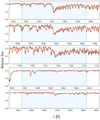 |
Fig. 7 Same as Fig. 6, but for the TiO γ and ϵ bands. |
| In the text | |
|
Fig. 8 Central prior Teff and log g values for the sample following Cifuentes et al. (2020). The spectral types are colour-coded. The dashed black line is the average Teff and log g for K7 V to M9.0 V objects, with the corresponding uncertainties shaded in grey. The 15 outliers discussed in Sect. 3.4 are labelled and listed in Table 4. Two and three stars are superimposed under labels (7) and (11), respectively. |
| In the text | |
|
Fig. 9 Interpolation scheme between Z and [Fe/H] in alpha-enhanced (red) and alpha-solar (black) models. |
| In the text | |
|
Fig. 10 Comparison between this work and the VIS+NIR analysis done by Passegger et al. (2019). Spectral types are colour-coded. The dashed black lines indicate the 1:1 relationship. |
| In the text | |
|
Fig. 11 Kiel diagram of the sample showing the parameters computed with STEPARSYN. Squares depict Hα-active stars. The metallicity [Fe/H]corr is colour-coded. Lines correspond to 5-Ga PARSEC isochrones with [Fe/H] = −0.4, 0.0, and 0.2 dex (Bressan et al. 2012). Typical uncertainties in logg and Teff are shown in the bottom-right corner. Outliers in logg are marked with red and blue circles (see Sect. 4 for details). |
| In the text | |
|
Fig. 12 Comparison of Teff (top panel) and [Fe/H] (bottom panel) between the runs with free and fixed log g. The quantity Δlogg is calculated as logg (prior) − logg (free). |
| In the text | |
|
Fig. 13 Metallicity distribution in this work and in the Geneva-Copenhagen survey (Nordström et al. 2004). |
| In the text | |
|
Fig. 14 M-dwarf metallicity distributions separated by the kinematic membership of the targets in the thick disc (TD), the thick disc-thin disc transition (TD-D), the thin disc (D), and the young disc (YD), following Cortés-Contreras et al. (in prep.). The vertical dashed lines indicate the peak of the distributions. |
| In the text | |
|
Fig. 15 Comparison in Teff (upper panel) and logg (bottom panel) for M dwarfs with interferometric angular measurements (see Table 6). The dashed black lines indicate the 1:1 relationship, whereas the dotted red lines show the 1:1 relationship, shifted following the average differences in each parameter. The blue shaded region denotes the 1σ level. |
| In the text | |
|
Fig. 16 Same as Fig. 15, but for the comparison in [Fe/H] between the components in FGK+M (blue) and M+M (red) systems (see Tables 7 and 9). |
| In the text | |
|
Fig. A.1 Same as Fig. 5, but for GX And (M1.0 V, J00183+440). The retrieved parameters are Teff = 3603 ± 24 K, log g =4.99 ± 0.14 dex, and [Fe/H] = −0.75 ± 0.11 dex. |
| In the text | |
|
Fig. A.2 Same as Fig. 5, but for Luyten’s star (M3.5 V, J07274+052). The retrieved parameters are Teff = 3380 ± 43 K, log g =4.96 ± 0.11 dex, and [Fe/H] = −0.17 ± 0.11 dex. |
| In the text | |
|
Fig. A.3 Same as Fig. 5, but for Teegarden’s star (M7.0 V, J02530+168). The retrieved parameters are Teff = 3034 ± 45 K, log g =5.19 ± 0.20 dex, and [Fe/H] = −0.17 ± 0.28 dex. |
| In the text | |
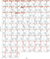 |
Fig. A.4 Same as Fig. 6, but for GX And (M1.0 V, J00183+440). |
| In the text | |
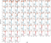 |
Fig. A.5 Same as Fig. 6, but for Luyten’s star (M3.5 V, J07274+052). |
| In the text | |
 |
Fig. A.6 Same as Fig. 6, but for Teegarden’s star (M7.0 V, J02530+168). |
| In the text | |
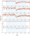 |
Fig. A.7 Same as Fig. 7, but for GX And (M1.0 V, J00183+440). |
| In the text | |
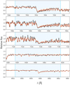 |
Fig. A.8 Same as Fig. 7, but for Luyten’s star (M3.5 V, J07274+052). |
| In the text | |
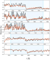 |
Fig. A.9 Same as Fig. 7, but for Teegarden’s star (M7.0 V, J02530+168). |
| In the text | |
|
Fig. A.10 Comparison between this work and Rojas-Ayala et al. (2012). |
| In the text | |
|
Fig. A.11 Comparison between this work and Gaidos & Mann (2014). |
| In the text | |
|
Fig. A.12 Comparison between this work and Maldonado et al. (2015). |
| In the text | |
|
Fig. A.13 Comparison between this work and Mann et al. (2015). |
| In the text | |
|
Fig. A.14 Comparison between this work and Passegger et al. (2018). |
| In the text | |
|
Fig. A.15 Comparison between this work and Rajpurohit et al. (2018a). |
| In the text | |
|
Fig. A.16 Comparison between this work and Schweitzer et al. (2019). |
| In the text | |
|
Fig. A.17 Comparison between this work and Maldonado et al. (2020). |
| In the text | |
|
Fig. A.18 Comparison between this work and Passegger et al. (2020). |
| In the text | |
Current usage metrics show cumulative count of Article Views (full-text article views including HTML views, PDF and ePub downloads, according to the available data) and Abstracts Views on Vision4Press platform.
Data correspond to usage on the plateform after 2015. The current usage metrics is available 48-96 hours after online publication and is updated daily on week days.
Initial download of the metrics may take a while.