| Issue |
A&A
Volume 656, December 2021
|
|
|---|---|---|
| Article Number | A108 | |
| Number of page(s) | 10 | |
| Section | Extragalactic astronomy | |
| DOI | https://doi.org/10.1051/0004-6361/202141869 | |
| Published online | 09 December 2021 | |
First black hole mass estimation for the quadruple lensed system WGD2038-4008
1
Instituto de Físisca y Astronomía, Facultad de Ciencias, Universidad de Valparaíso, Av. Gran Bretaña 1111, Valparaíso, Chile
e-mail: This email address is being protected from spambots. You need JavaScript enabled to view it.
2
Núcleo Milenio de Formación Planetaria – NPF, Universidad de Valparaíso, Av. Gran Bretaña 1111, Valparaíso, Chile
3
European Southern Observatory, Alonso de Córdova 3107, Vitacura, Santiago, Chile
4
Núcleo de Astronomía de la Facultad de Ingeniería y Ciencias, Universidad Diego Portales, Av. Ejército Libertador 441, Santiago 8320000, Chile
5
Instituto de Astrofísica de Canarias, Vía Láctea s/n, La Laguna, 38200 Tenerife, Spain
6
Departamento de Astrofísica, Universidad de la Laguna, La Laguna 38200 Tenerife, Spain
7
Harvard-Smithsonian Center for Astrophysics, 60 Garden St., Cambridge, MA 02138, USA
Received:
23
July
2021
Accepted:
30
September
2021
Abstract
Context. The quadruple lensed system WGD2038-4008 (zs = 0.777 ± 0.001) has recently been discovered with the help of new techniques and observations. Black hole masses have been estimated for lensed quasars, but they have mostly been calculated for one broad emission line of one image. However, the images could be affected by microlensing, which changes the results.
Aims. We present black hole mass (MBH) estimations for images A and B of WGD2038-4008 using the three most prominent broad emission lines (Hα, Hβ, and Mg II) obtained in one single-epoch spectra. This is the first time the mass has been estimated in a lensed quasar in two images, allowing us to disentangle the effects of microlensing. The high S/N of our spectra allows us to get reliable results that can be compared with the existing data in the literature.
Methods. We used the X-shooter instrument mounted on the Very Large Telescope at Paranal Observatory to observe this system, taking advantage of its wide spectral range (UVB, VIS, and NIR). The sky emission correction was performed using principal component analysis as the nodding was small compared to the image separation. We compared the lines profiles to identify the microlensing in the broad-line region and corrected each spectra by the image magification. Using the flux ratio of the continuum to the core of the emission lines, we analyzed whether microlensing was present in the continuum source.
Results. We obtained MBH using the single-epoch method with the Hα and Hβ emission lines from the monochromatic luminosity and the velocity width. The luminosity at 3000 Å was obtained using the spectral energy distribution of image A, while the luminosity at 5100 Å was estimated directly from the spectra. The average MBH between the images obtained was log10(MBH/M⊙) = 8.27 ± 1.05, 8.25 ± 0.32, and 8.59 ± 0.35 for Mg II, Hβ, and Hα, respectively. We find Eddington ratios similar to those measured in the literature for unlensed low-luminosity quasars. Microlensing of −0.16 ± 0.06 mag in the continuum was found, but the induced error in the MBH is minor compared to that associated with the macromodel magnification. We also obtained the accretion disk size using the MBH for the three emission lines, obtaining an average value of log10(rs/cm)=15.3 ± 0.63, which is in agreement with theoretical estimates.
Key words: gravitational lensing: strong / gravitational lensing: micro / quasars: individual: WGD2038-4008 / black hole physics / quasars: supermassive black holes
© ESO 2021
1. Introduction
The number of lensed quasars discovered is consistently growing thanks to the help of new identification techniques and observations (Agnello et al. 2018; Krone-Martins et al. 2019; Lemon et al. 2020). Here, we study one of these recently identified lenses, WGD2038-4008. This system is a quadruple lensed quasar discovered in 2017 using a combination of Wide-field Infrared Survey Explorer (WISE, Wright et al. 2010) and Gaia (Gaia Collaboration 2016) over the Dark Energy Survey (DES, Dark Energy Survey Collaboration 2016) footprint with a source and deflector redshift of zs = 0.777 ± 0.001 and zl = 0.230 ± 0.002 respectively (Agnello et al. 2018). The deflector is a red galaxy with a compact bulge and a bright halo while the source has an extended quasar host galaxy (Agnello et al. 2018). It was observed using the Hubble Space Telescope (HST) obtaining a lens model for this system (Shajib et al. 2019) using LENSTRONOMY (Birrer & Amara 2018). Spatially resolved narrow-line fluxes ([OIII] in Nierenberg et al. 2020) are also available. Buckley-Geer et al. (2020) studied the lensing galaxy to measure its velocity dispersion and to identify the line-of-sight galaxies that need to be included in the lens model. Even though gravitational lensed quasars are a powerful tool for studying the inner structure of active galactic nuclei (AGNs; Pooley et al. 2007; Anguita et al. 2008; Poindexter et al. 2008; Dai et al. 2010; Morgan et al. 2010; Treu 2010; Jiménez-Vicente et al. 2014; Motta et al. 2017), no such study has been conducted to date for WGD2038-4008. One of the difficulties of working with lensed quasars is that microlensing can affect different regions of the broad emission lines (BELs) in the spectra of one or more images of the system (Mediavilla et al. 2011; Motta et al. 2012; Guerras et al. 2013; Fian et al. 2018; Rojas et al. 2020). Microlensing can affect the observed flux of the accretion disk and the BELs, as well as the shape of the BELs, ultimately adding uncertainty to the single-epoch black hole mass (MBH) estimation.
Precise measurement of the MBH is key to understanding the coevolution between the supermassive black hole (SMBH) growth and the host galaxy (see Ferrarese & Ford 2005; Kormendy & Ho 2013). In particular, physical parameters of the SMBH seem to correlate well with the luminosity (Marconi & Hunt 2003) and velocity dispersion (Ferrarese & Merritt 2000; Tremaine et al. 2002) of the host galaxy.
The single-epoch (SE) method is one of the most widely used technique to measure MBH in AGNs: it relates the continuum luminosity of the quasar at a particular wavelength with the size of the broad-line region (BLR; see Vestergaard 2004; Shen & Liu 2012; Mejía-Restrepo et al. 2016). Typically, the SE masses for low-redshift quasars (z < 0.7) are estimated in the optical using Hα and Hβ BELs and the continuum luminosity at 5100 Å. However, the Balmer lines are shifted into the infrared at higher redshifts, thus most of the estimations have been measured in the UV wavelength using Mg II and CIV BELs. Over the last decade, the SE method has been used to obtain MBH in lensed AGNs (Peng et al. 2006; Greene et al. 2010; Assef et al. 2011; Sluse et al. 2012; Mediavilla et al. 2018), but most of them from the Mg II and CIV BELs, and none of them using different emission lines observed simultaneously.
In this paper we present high signal-to-noise ratio (S/N) SE spectra for the quadruple lensed system WGD2038-4008 to obtain the MBH for three emission lines (Hα, Hβ, and Mg II) for two of the images. We also study microlensing in the emission lines and in the continuum, and finally we obtain the velocity dispersion of the lensing galaxy.
The paper is organized as follows. In Sect. 2 we present the data along with the reduction and the extraction of the spectra for each component. Section 3 shows the description of the method used for the estimation of the MBH, microlensing analysis, and velocity dispersion of the lensing galaxy. We present our results in Sect. 4 comparing with previous studies of different lensed quasars and finally our conclusions are presented in Sect. 5. We assume a Lambda cold dark matter (ΛCDM) cosmology with: ΩΛ = 0.7, ΩM = 0.3 and HO = 70 km s−1 Mpc−1.
2. Observation and data reduction
2.1. Observational strategy
We obtained spectra for WGD2038-4008 during July 2019 as part of ESO proposal ID 103.B-0566(A) (PI: A. Melo) using the X-shooter instrument mounted at the 8.2 m UT2 at the Very Large Telescope (VLT), Paranal Observatory, Chile (Vernet et al. 2011). X-shooter is a medium-resolution spectrograph that observes in a wide spectral range, from ultraviolet (UVB; 3000–5600 Å), through visible (VIS; 5500–10200 Å), and up to the near-infrared (NIR; 10200–24800 Å). We used three observing blocks (OBs) taken on two different nights with an average seeing of 1.12″. The UVB slit was 1.0″ × 11″ (spectral resolution R = 5400), while the VIS and NIR slits were 1.2″ × 11″ (R = 6500 and 4300, respectively) with a readout mode (UVB and VIS) of 100k/1pt/hg and a nodding of 3″ per individual frame. Each UVB/VIS (NIR) OB consists of 2 (4) exposure frames. The atmospheric dispersion corrector (ADC) is used to avoid chromatic differential atmospheric refraction. Table 1 summarizes the main observational characteristics of WGD2038-4008.
Log of the observation for the three observing blocks.
The slit position was chosen to cover the two brightest source images, centered on image B of the gravitational lensed quasar with a position angle on the sky of 126.8514° to include image A (see Fig. 1).
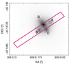 |
Fig. 1. Scheme of the slit position centered on image B (RA 307.5115875, DEC -40.13736167, epoch J2000) of WGD2038-4008. The FITS image is from the Dark Energy Survey in filter r (Gravitational Lensed Quasar Database https://research.ast.cam.ac.uk/lensedquasars/). |
2.2. Data processing
We used the ESO pipeline EsoReflex (Freudling et al. 2013) workflow with the X-shooter pipeline version 3.5.0 to reduce each OB without using nodding to subtract the sky emission. This method was employed instead of the standard model because the 3″ nodding is comparable to the image separation (∼2.87″), which causes a self-subtraction flux from the lensed quasar spectra. The next steps in the reduction and extraction were slightly different for the three arms of the instrument. Once the frames were corrected by cosmetics (flat field, dark current, wavelength calibration, among others), we proceeded to subtract the sky emission in the NIR arm. We designed a sky emission correction for each individual frame based on principal component analysis (PCA, Deeming 1964; Bujarrabal et al. 1981; Francis & Wills 1999), a method normally used in multi-dimensional analysis. PCA uses a basis of eigenvectors that are constructed to describe the data (e.g., by maximizing the variance of the projected data). This method is usually applied to reduce the number of parameters describing a data set by computing the principal components to change the representation of the data. The number of components used in the reconstruction was chosen to minimize the standard deviation of the residuals between the spectrum and all sky models (using a different number of components). The procedure used to obtain the best representation of the underlying sky emission in each frame consists of the following steps. First, we masked the outliers (such as bad pixels) using σ-clipping (σ = 5 with three iterations), replacing them with an estimated value obtained from a bicubic interpolation using the surrounding pixels. Then, we calculated the median for each wavelength bin to obtain a rough approximation of the sky emission as a function of the wavelength. We note that this value is only used to identify the targeted spectra (quasar lensed images A and B, as well as the lens galaxy). We subtracted this rough sky median from each frame and collapsed the remaining 2D spectra along the wavelength (see Fig. 2 right and left, respectively) to select an uncontaminated spatial region for the sky emission. A threshold equal to 3 pixels, above and below the dispersion of the median, above the background (see Fig. 2, left) is applied to choose the region to be employed as the PCA-basis (normalized to the unit). The PCA eigenvector basis is obtained by constructing a model of the sky emission in the selected spatial region. This 2D sky model is then subtracted from the frame.
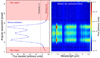 |
Fig. 2. Two-dimensional spectra for WGD2038-4008. Left: collapsed frame along the wavelength axis after the subtraction of the sky median. The pink shaded zone represent the sky region (see text below). Right: NIR frame after sky subtraction. |
Flux calibration is done by using the response curve from the end-products of the X-shooter pipeline. This response is obtained from a standard star observed the same night as the target, in our case GD153, EG 274 and Feige 110 for OB 1, 2, and 3, respectively.
After the sky modeling and subtraction, we employed molecfit (Smette et al. 2015; Kausch et al. 2015) in each frame to correct by telluric absorptions. For each frame, the target spectra were median-combined into a single spectrum in order to increase the signal and decrease the noise. The spatial region occupied by the targets was previously calculated during the PCA sky emission estimation, and corresponds to the source emission region in Fig. 2. The molecfit best fit was applied to each frame row by row. Once the frames were corrected by sky emission and telluric absorption, they were median combined and the uncertainties estimated as the median absolute deviation. All the parameters required for the stacking (e.g., dittering, pixel scale) were obtained from the header of each frame, modified by the X-shooter workflow. Figure 3 shows the result of the final 2D spectrum (top panel) compared to that obtained as end-product from the ESO pipeline (bottom panel).
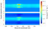 |
Fig. 3. Final 2D NIR spectrum using the PCA sky extraction described in Sect. 2.2 (top) compared to the one using ESO pipeline reduction (bottom). Both spectra are flux calibrated and telluric corrected. |
In contrast to the NIR, the VIS observations are not dominated by the sky brightness. Therefore, instead of the PCA analysis, we used the median of each sky region as the best representation of the sky brightness, obtained in the same way as for the NIR (selecting a region free of source emission to compute the sky brightness representation). The flux calibration, telluric correction, and combination of frames are done in the same way as for the NIR arm. Even though the UVB arm does not require sky subtraction, we used the same procedure as the VIS arm to be consistent with the reduction.
2.3. One-dimensional extraction
Due to the small separation between the quasar images A, B, and the lens galaxy, there can be cross-contamination in their spectra (see Fig. 1). To obtain uncontaminated spectra we proceeded as follows. First, we collapsed the 2D reduced spectrum along the wavelength axis in a high S/N region, for example around an emission line region (Hα in the NIR, OIII in VIS, and Mg II in the UVB arm). In the case of the VIS and UVB arms, we selected bins of 20 pixels (4 Å) to increase the S/N of the sources. We masked the outliers (persistent bad pixels, poor sky subtraction, and/or low S/N regions) to obtain the best-fit parameters as a function of the wavelength. The spatial contribution of each component was estimated by simultaneously fitting three Gaussian profiles. The distances between image A and B (∼2.87 arcsec ≈14 pixels) and between image A and the lens galaxy projection onto the AB segment (∼1.47 arcsec ≈8 pixels) were used to fix the position of the Gaussian centers for B and the lens galaxy, respectively. Assuming A and B are point sources, we can consider that they have the same full width at half maximum (FWHM) and standard deviation parameter (σ), and a variable σl (larger than σ, due to its extended emission) for the lensing galaxy in the UVB and VIS arms. Due to the faintness of the lens galaxy in the NIR arm, the σl value of the lens galaxy is considered the same as for the images (σl = σ). Thus, the free parameters are the amplitudes, image A center, σ for the point sources (and lens galaxy in NIR), and σl for the lens galaxy (in the UVB and VIS arms). Using the best-fit estimated values and their respective uncertainties, we constructed a probability function for the spatial distribution of each target (quasar images and lens galaxy), allowing us to identify the probability that a given spatial pixel belongs to one of the targets. We used error propagation for each free parameter to estimate the related uncertainties in each final uncontaminated spectrum.
Considering the seeing variation along the wavelength range and the selected slit width, we needed to estimate the percentage of lost flux. We estimated the broadening of the spectra profile due to the instrumental dispersion at different wavelengths by fitting a Gaussian function for each wavelength bin of the telluric standard star (HD 115470 for the case of OB 1 of seeing 0,75″). The σ⊙ obtained was of 0.76″ with a dispersion that does not vary from 1 pixel between the arms. We used this value (see in Table 1) to calculate the percentage of flux entering the slit by simulating the system as a sum of the Gaussian functions and sigma obtained from the header and integrating it within the slit using the seeing delivered in the header. The percentage of flux lost was 30.5% in UVB, 14.9% in VIS, and 19.74% in NIR. These values will be included as an extra flux error in all our analyses.
After extracting the spectra for the three components, we found that the lens galaxy spectrum shows contamination by quasar emission lines. Given the amount of contamination, the slit width and position angle, we infer that this is a contribution from image C (see Fig. 1). To obtain the uncontaminated lens galaxy spectrum, we used spectrum A as a proxy for C and estimated the C contribution fraction for each arm (0.25 for NIR, 0.43 for VIS, and 0.5 for UVB) that removes the quasar emission lines. The S/N of the emission line and continuum were obtained by estimating the standard deviation of the background. We used the 2D spectra to obtain the background emission (sky emission in Sect. 2.2), getting the mean and standard deviation of this background. We then chose a continuum region located around the emission line (50 Å) for each signal contribution (image A, B, and the lensing galaxy) and obtained the mean value. With these values we calculated the S/N of the continuum. We calculated the S/N of the emission lines using the same method: selecting the same spatial region, but estimating the mean in a reduced wavelength window (approximately 300–500 Å) around each emission line. The S/N values for the continuum and emission lines are listed in Table 2.
FWHM, luminosities, and MBH.
The final spectra for images A, B, and the lensing galaxy (uncontaminated by the quasar emission) are presented in Fig. 4. As the ADC did not work during the night that OB 1 and 2 were taken, the UVB and VIS arm experienced flux loss (Fig. 4), explaining the atypical profile of the AGN spectra (see Vanden Berk et al. 2001 and Glikman et al. 2006 for a composite quasar spectra). This loss will affect the luminosity measurement, specially in the UVB arm (see Sect. 3.1 for more details).
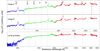 |
Fig. 4. Rest-frame X-shooter spectra for image A, image B, and the lensing galaxy. The different arms of the instrument are shown: UVB (green), VIS (blue), and NIR (red). The images are corrected by their respective redshifts (zs = 0.777 and zl = 0.230). The atmospheric windows are left blank for the NIR band. The lensing galaxy is uncontaminated by the quasar emission. The wavelength is in the rest frame of the respective object and the position of the emission lines are shown as dashed lines. |
3. Methods
Black hole mass is estimated by using the SE method (e.g., McLure & Dunlop 2004; Shen et al. 2008; Trakhtenbrot & Netzer 2012), which combines the Doppler line width of the broad emission line and the monochromatic luminosity to obtain a proxy for MBH. If we assume that the emitting gas in the BLR is virialized, then
 (1)
(1)
where G is the gravitational constant, RBLR is the BLR size, (Δv)2 is the velocity of the line emitting gas in the BLR, and f is the virial factor that depends on the unknown structure, kinematics, inclination, and distribution of the BLR (Peterson et al. 2004 and references therein). The BLR size comes from the reverberation mapping (RM, Blandford & McKee 1982; Peterson 1993) and from the known correlation between the AGN luminosity and the size of the BEL, RBLR ∼ (λLλ)α (e.g., Kaspi et al. 2000, 2005; Bentz et al. 2009), allowing us to estimate MBH as
 (2)
(2)
where K = G−1f. The literature shows different values for the parameters K and α (McLure & Dunlop 2004; Vestergaard & Peterson 2006; Vestergaard & Osmer 2009; Shen et al. 2011), although we use those estimated by Mejía-Restrepo et al. (2016) because they were estimated using a similar observing setup, thus minimizing the systematic effects. In particular, the sample of Mejía-Restrepo et al. (2016) contains several emission lines for each object; in addition all the lines for a single object were observed simultaneously. The values for the parameters used for the emission lines (Hα, Hβ, and Mg II) at their respective luminosities (L5100, L5100, L3000) are
(log K, α)Hα = (6.845, 0.650),
(log K, α)Hβ = (6.740, 0.650),
(log K, α)Mg II = (6.925, 0.609).
In addition to the usual uncertainties related to the SE method (FWHM, luminosity, and f parameter estimations), the observed source luminosity also needs to be corrected for the lensing magnification. To obtain the magnification factor (μ) we use the convergence (κ) and shear (γ) parameters estimated from the lens model as μ = 1/[(1 − κ)2 − γ2] (Narayan & Bartelmann 1996). Employing the values previously calculated by Shajib et al. (2019), we obtain a magnification factor of μA = 2.27 ± 0.21 and μB = 2.71 ± 0.32.
3.1. Emission line fitting and luminosity measurement
After demagnifying the spectra, and removing the continuum and the iron template (following Mejía-Restrepo et al. 2016), we modeled each emission line profile and estimated the BEL FWHM. We used Gaussian functions to represent the broad and narrow components of each emission line (see Table 4 of Shang et al. 2007) and masked those regions affected by absorptions1. In the Hα region we added four extra Gaussian components for the [N II] and [S II] narrow-line region (NLR) doublets. In the Hβ region we considered two extra Gaussians for the [O III] NLR doublet and one for the He II broad emission line. For the Mg II region we considered two narrow and two broad components. The FWHM used for the MBH measurement was obtained from the standard deviation of line profile after removing the NLR component (i.e., the resulting profile is the combined Gaussians representing the broad line components). The uncertainties were obtained using error propagation and a Monte Carlo simulation of 1000 random resamplings, assuming a Gaussian distribution for the flux uncertainty at each pixel. The best line fit is shown in red in Fig. 5. As every emission line exhibits some kind of distortion (possible absorptions) that could lead to an overestimation of their FWHM, we decided to mask those regions for the Gaussian fitting. The Mg II profile has several absorption features (masked region [2787:2794, 2796:2802] Å), possibly caused by the circumgalactic medium (CGM). In the case of Hα the feature perceived as absorption masked region [6525:6547, 6569:6576] Å could instead be a very bright NLR. Similarly, Hβ shows a distorted profile (masked region [4835:4849, 4866:4878] Å) possibly related to a poor FeII fitting. The monochromatic luminosity was measured using continuum windows on each side of the emission line ([4670: 4730, 5080: 5120] Å for Hβ and [6150: 6250, 6800: 6900] Å for Hα). These spectral windows were selected for the low (or even null) emission line contamination levels, and were used to interpolate the region of interest following a single power-law function. As mentioned above, the flux loss in the UVB and VIS arms impede the use of the spectra to estimate the monochromatic luminosity at 3000 Å. Instead, we estimated this luminosity by fitting a spectral energy distribution (SED) template of Assef et al. (2010) to the unmagnified magnitudes obtained from HST (Shajib et al. 2019) and DES (Agnello et al. 2018). Compared to the luminosity measurement, the FWHM of Mg II FWHM is not affected by this flux loss.
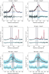 |
Fig. 5. Gaussian fitting of Hα, Hβ, and Mg II regions for images A (left) and B (right). The red line represents the best fit, the black lines represent the different components of each region (emission and absorption), the green line represents the Fe template, and the blue line is the continuum fit of the spectra. The 1σ error of the spectra along with the residuals and their respective errors are at the bottom of the images. |
The FWHM obtained from the line profile fitting and the monochromatic luminosity (estimated from the continuum and SED) for each emission line in image A and B is presented in Table 2.
3.2. Microlensing analysis
Microlensing can induce flux variations in the quasar images due to lensing from stars in the lensed galaxy halo (e.g., Chang & Refsdal 1979; Schneider et al. 2006). This flux variation in one or more images is sensitive to the angular size of the source, meaning that the magnification will be bigger for a smaller emitting region. In this situation, we could study the inner structure of WGD2038-4008 from the SE images of different observations, where the accretion disk and BLR can be affected differently by microlensing and could affect the wings of the emission lines. On the contrary, the NLR is insensitive to microlensing and can be used as the baseline (Abajas et al. 2002). To investigate whether microlensing is present, we use the magnitude difference between the emission line core and the continuum (see Moustakas & Metcalf 2003; Mediavilla et al. 2009, 2011; Motta et al. 2012, 2017; Guerras et al. 2013; Rojas et al. 2020). The quasar emission lines have different components, meaning that they come from different inner regions of the AGN. The line core is dominated by the NLR, while the wings are dominanted by the BLR emission. In addition, the light of each image follows a different path through the lens galaxy where gas and dust can produce extinction. We can separate microlensing from extinction considering that only the latter will affect both the continuum flux ratio and the core of the emission line (Falco et al. 1999; Motta et al. 2002; Mediavilla et al. 2005). We obtain the magnitude difference between components in the continuum by fitting a straight line between two regions on each side of each emission line. The regions are ∼30−40 Å in size. We integrated the line between the two regions to obtain the continuum flux for both images. This continuum is then subtracted from the spectrum and we integrate a small window (between 10–30 Å) centered in the emission line core to obtain the flux uncontaminated by the continuum. Integrating in the core of the emission line decreases the BEL contamination that can also be affected by microlensing. The uncertainty of the flux is assumed to be related to the continuum fitting and is obtained using error propagation, where the square root of the error in the spectra and the straight line are added in quadrature. Finally, the magnitude difference between image A and B for each region (continua and line cores) is mA − mB = −2.5log(FA/FB), obtaining a (mA − mB)line for the core of the emission line and a (mA − mB)cont for the continuum.
3.3. Stellar velocity dispersion of the lens galaxy
The stellar velocity dispersion (σ) of a galaxy measures the random motion of stars due to a presence of a mass. Obtaining an accurate dispersion value is important to restrict the lens model parameters, and together with the light curves of the images of the lensed quasar measure the Hubble constant H0 and helps to improve the uncertainties. The velocity dispersion was estimated from the lens galaxy spectrum using the penalized pixel-fitting (pPXF; Cappellari & Emsellem 2004; Cappellari 2017). We used the rest-frame wavelength 3600–4200 Å for the UVB arm and 4800–5800 Å for the VIS arm. The spectra were fitted using the Single Stellar Population library by Vazdekis et al. (2010) included in pPXF (see Fig. 6). The velocity dispersion obtained was 299 ± 12 km s, consistent with the measurements of Buckley-Geer et al. (2020) (296 ± 19 km s and 303 ± 24 km s using Gemini South/GMOS-S spectra).
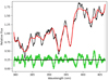 |
Fig. 6. Fit of stellar templates to the lensing galaxy using pPXF package after removing the extra quasar contribution. |
4. Results
We identified the three most prominent emission lines of the lensed quasar (Mg II, Hβ, and Hα) with high S/N (see Table 2). The spectra were demagnified using the parameters from the lens model of Shajib et al. (2019) and the continuum was subtracted to compare the profiles of image A and B (Fig. 7). Interestingly, we find an enhancement of the right wing of Hα emission line of image B compared to image A (between ∼6600 and 6700 Å). This magnitude difference (∼0.28 ± 0.03 mag integrated in the region [6591.4:6686.5] Å) could be explained assuming that microlensing is affecting the Hα broad emission line. This effect should also be seen in the Hβ profile as it arises from a region of similar size to Hα. However, we do not detect this effect, although this could be due to the low S/N of Hβ (S/N ⪅ 20) compared to Hα (S/N ⪆ 72) and to the presence of absorption-like features. There is no sign of this effect in the Mg II profile (S/N ⪅ 31), which is reasonable because Mg II emission is produced in a region farther away than the Balmer lines (Goad et al. 2012), and hence is less susceptible to microlensing effects.
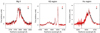 |
Fig. 7. Mg II, Hβ, and Hα emission line region. The images are demagnified using the magnification values given in Sect. 3. |
Multi-Gaussian fitting of images A and B are shown in Fig. 5 following the procedure described in Sect. 3.1. The gray shaded regions represent the masked sections used during the fitting. Table 2 shows the FWHM estimated for each broad emission line in each quasar image. Even though the components of Mg II have slightly different amplitudes, probably due to the absorptions that are contributing to the profile, the FWHM values are within the errors. The FWHM of Hβ is in good agreement in spite of the low S/N. In the case of Hα,the estimated FWHM is different (> 5σ) and we discuss below how this might affect our MBH estimations. To investigate whether microlensing is present in the continuum, we obtained the magnitude difference between the core of each emission line uncontaminated by the continuum, (mA − mB)line, and the continuum under the emission line, (mA − mB)cont, shown in Fig. 8. The Hα emission line region shows two values corresponding to two emission line peaks, avoiding the right wing (see Fig. 7), integrated in the windows [6500.1:6526.0, 6547.7:6565.4] Å. The Hβ region shows three values corresponding to Hβ ([4820:4890] Å integration window) and the [OIII] doublet emission line cores ([4949.2:4960.0, 4996.4:5007.0] Å integration window). We included the Mg II region integrated between [2774.6:2784.1] Å and Paschenϵ [9512.0:9533.0] Å. Considering that the magnitude difference in the emission lines is approximately constant, we use the median and its standard error, (mA − mB)line = 0.17 ± 0.05 mag, as our baseline of no-microlensing. As the values for the integrated continuum also yield a roughly constant value along the wavelength, we use the median to estimate (mA − mB)cont = 0.01 ± 0.03 mag. We compare our result with spectroscopic data of the integrated flux obtained by Nierenberg et al. (2020) (see Fig. 8)  and
and  mag, which is in agreement with our magnitude difference for the continuum and emission line in the Hβ region, respectively. Published data from broadband photometry taken between 2016 and 2017 is also included in Fig. 8 (Agnello et al. 2018; Lee 2019; Shajib et al. 2019). We fit a median function to these values obtaining (mA − mB)lit = 0.21 ± 0.06 mag. The values are in agreement with the core of our narrow emission lines.
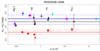 |
Fig. 8. Magnitude difference mA − mB vs. λ0 between images A and B. The red squares show the integrated continuum and the black circles the emission line core without the continuum using X-shooter. Shown are the measurements obtained from the literature: HST (Shajib et al. 2019) (magenta triangles), VISTA (Lee 2019) (cyan diamonds), DES (Agnello et al. 2018) (blue diamonds) and HST F105W/G102 (Nierenberg et al. 2020) (orange square for continuum and orange triangle for a narrow emission line). The red line is the median of the continuum, the dotted red line the standard deviation, the black line the emission line core, and the blue line the literature. |
Since the above-mentioned data are not time-delay corrected, the magnitude difference estimated from our spectra, Δm = (mA − mB)cont − (mA − mB)line = −0.16 ± 0.06 mag, could be due to intrinsic variability coupled with a time lag between the images. We use the Yonehara et al. (2008) procedure to estimate this effect. We assume the structure function inferred from the imaging data of quasars (Vanden Berk et al. 2004), an absolute magnitude range for the source in I band, MI = (−21, −30), the predicted time delay for the quasar images ΔtAB = −6 ± 1 days (Shajib et al. 2019), and assume no lag between our observations as they were obtained with 1 day of difference. We obtained a magnitude difference induced by time delay coupled with intrinsic variability of 0.05 mag (0.03 mag) to 0.07 mag (0.04 mag) for a −21. mag (−30. mag) source in the F160W and F475W HST broadband filters, respectively. On the other hand, we also use light curves obtained by COSMOGRAIL (e.g., Bonvin et al. 2017; Courbin et al. 2011; Eigenbrod et al. 2005), which has a monitoring program to obtain time delay between multiple images of lensed quasars. WGD2038-4008 follow-up is carried out in MPIA 2.2m telescope (La Silla Observatory, Chile) with an average of one measurement per week (F. Courbin, priv. comm.), although no time delay has been measured yet. We considered three dates that were seven days apart and within two weeks of our X-shooter observations, then shift the B data to correct by time delay, and estimate the average magnitude difference as (mA − mB)corr ∼ 0.16 ± 0.03 mag. This value is in good agreement with our estimation using the core of the emission lines. Therefore, Δm = −0.16 ± 0.06 mag seems to indicate the presence of a constant or long-lasting microlensing event not detected by the light curves (Sluse & Tewes 2014). To investigate this possibility, we estimate the timescale associated with such event. Following Treyer & Wambsganss (2004), we define two timescales: the standard lensing time (tE), and the crossing time (tcross). The first represents the time it takes a star to cross a length equivalent to the Einstein radius
 (3)
(3)
where zL is the lens redshift, RE the Einstein radius in the source plane, and v⊥ the effective source velocity (Treyer & Wambsganss 2004). The second timescale refers to the time, within the length of an Einstein radius, when the source may encounter a caustic line, causing a large magnification
 (4)
(4)
where Rsource is the quasar size (i.e., the accretion disk size, log10(rs/cm) = 15.65), and DS and DL the angular diameter distance (Hogg 1999) of the observer-source and observer-lens, respectively, with our assumed cosmology. Considering a typical value of v⊥ = 600 km s−1 as assumed by Treyer & Wambsganss (2004), we estimate tE ≃ 27.7 years and tcross ≃ 0.6 year. On the other hand, if we calculate the effective source velocity following Mosquera & Kochanek (2011) 2, we obtain veff = 820 km s−1, which yields tE ∼ 20.3 years and tcross ≃ 0.5 year, respectively. Thus, a long-lasting microlensing event would last for ∼20 years, while the crossing time should be around 6 months.
In spite of this microlensing magnification, the induced error in the luminosity is negligible as the majority of the error budget is introduced by the macro model magnification (Sect. 3).
The monochromatic luminosity at L5100 was estimated using a single power-law function between two continuum windows on each side of the BELs. It agrees for Hα and Hβ of each image, within the errors, with an average value of log10(L5100/L⊙) = 44.29 ± 0.03. Due to flux loss in UVB, we modeled a SED to estimate L3000 using the magnitudes and magnification of image A, obtaining log10(L3000/L⊙) = 44.23 ± 0.19. The luminosities L300 and L5100 agree within their errors, even though they were obtained with different methods. The MBH was obtained following Eq. (2) with an average value between images A and B of log10(MBH/M⊙) = 8.59 ± 0.35, 8.25 ± 0.32, 8.27 ± 1.06 for Hα, Hβ, and Mg II, respectively. The MBH estimates obtained using the three different emission lines are consistent within 2σ. We show the MBH estimations along with those of the literature of lensed quasars in Fig. 9. To avoid the discrepancies associated with the different parameter values used by the authors, we combine their FWHM and monochromatic luminosity values using Eq. (2) to obtain MBH. We converted from intrinsic to bolometric luminosity applying Lbol = A Lref, where A = (3.81, 5.15, 9.6) for Lref = (L1350, L3000, L5100) presented in Sluse et al. (2012). MBH estimates for 33 lensed quasars are also included in Fig. 9 (some of them have several values as they are obtained from different emission lines) as well as those of Shen et al. (2019) for non-lensed quasars from SDSS reverberation mapping. The figure shows that our results for image A and B of WGD2038-4008 are in good agreement with those of the non-lensed quasars, situating our object in the low-luminosity range of the diagram.
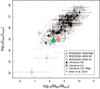 |
Fig. 9. MBH vs. Lbol for quasars. The masses plotted are estimated from different emission lines and monochromatic luminosity found to date (Peng et al. 2006; Assef et al. 2011; Sluse et al. 2012; Ding et al. 2017). For lensed quasars, black open diamonds correspond to the MBH derived from the Mg II and CIV emission lines, black open triangle correspond to the Hα emission line, and black filled triangles to the Hβ emission line. For non-lensed quasars, Shen et al. (2019) data for MBH from SDSS are represented by the gray dots and gray contours. The average MBH mass estimation for WG2038-4008 is represented as blue, red, and green triangles for Mg II, Hβ, and Hα emission lines. |
We can also infer the accretion disk size (rs) assuming a thin-disk model (Shakura & Sunyaev 1973) and considering our MBH estimate (Mosquera & Kochanek 2011) as
![Mathematical equation: $$ \begin{aligned} r_s= 9.7 \times 10^{15} \left( \frac{\lambda _{\rm rest}}{\upmu \mathrm{m}}\right)^{4/3} \left( \frac{M_{\rm BH}}{10^9 M_{\odot }} \right)^{2/3} \left( \frac{L}{\eta L_E} \right)^{1/3} {[\mathrm {cm}]} \end{aligned} $$](/articles/aa/full_html/2021/12/aa41869-21/aa41869-21-eq7.gif) (5)
(5)
Here λrest is the wavelength where the MBH is measured, η is the accretion efficiency, and L/LE the luminosity in units of the Eddington luminosity. For a typical accretion rate η = 0.1 and L/LE ∼ 1/3 (Schulze & Wisotzki 2010). Using the different MBH estimates with the wavelength value at Hα, Hβ, and Mg II, the accretion disk size measurements are shown in Table 2. The size of Mg II is on average log10(rs/cm) = 14.98 ± 0.84, Hβ is 15.25 ± 0.4, and Hα 15.67 ± 0.74. Our estimates are in agreement within each other and with Morgan et al. (2018). We scaled our wavelength (λ in which the MBH was measured) to 2500 Å, assuming rs ∝ λ4/3 and obtained log10(rs/cm) = 14.94 ± 0.22, 15.25 ± 0.82 and 15.65 ± 0.79 in Mg II, Hβ, and Hα, respectively. These values are consistent with the theoretical values estimated by Morgan et al. (2018) at r2500: 15.41 ± 0.15 for Mg II, 15.37 ± 0.26 for Hβ, and 15.62 ± 0.18 for Hα.
5. Conclusions
We obtained high S/N observations for the quadruple lensed system WGD2038-4008 using the X-shooter instrument at VLT. We used Gaussian fitting to obtain uncontaminated spectra for the A and B lensed quasar images and the lens galaxy. The most prominent emission lines were detected (Mg II, Hβ, and Hα) as well as the absorption lines in the lensing galaxy. We confirmed the velocity dispersion of the lensing galaxy spectra, obtaining 299 ± 12 km s−1, in agreement with previously estimated values (2.96 ± 19 km s−1Buckley-Geer et al. 2020).
The magnification factors were estimated from the lens parameters of Shajib et al. (2019) (μA = 2.27 ± 0.21 and μB = 2.71 ± 0.32) and were used to demagnify the spectra. Comparing the continuum-subtracted emission lines, we find that there is an enhancement in the right wing of Hα of image B that could be due to microlensing. However, this effect is not seen in Hβ (a region similar in size to Hα) but this might because of the low S/N and to the presence of absorption-like features. The Mg II profile does not show any sign of microlensing, and it could be because it is produced in a region that is farther away. Magnification in the red wing of the Hα broad emission line has been detected in HE0435-1223 (Braibant et al. 2014) and QSO2237+0305 (Braibant et al. 2016). The main conclusion is that these line profile distortions can be explained by the differential magnification of a Keplerian disk model. As the continuum region is expected to be smaller than the BLR, the profile distortions are also accompanied by larger magnification of the continuum. However, in our case the magnification in the continuum is smaller than that in the Hα broad emission line. On the other hand, several papers describe an enhancement in the Fe Kα profile with higher magnification than the X-ray continuum in MG J0414+0534 (Chartas et al. 2002), QSO 2237+0305 (Dai et al. 2003), and H1413+117 (Chartas et al. 2004). This effect is attributed to differential microlensing. Popović et al. (2003), who use a standard accretion disk and caustic crossing to investigate the structure that could lead to such differences, conclude in Popović et al. (2006) that different dimensions for the emitting region (e.g., an inner BEL anulus radius smaller than the continuum disk) and the segregation of emitters allow the reproduction of the Fe Kα enhancement without an equivalent amplification of the continuum. Furthermore, Abajas et al. (2007) demonstrated that this result could also be obtained in the case of a biconic model for the BEL. Thus, a similar effect might be used to explain our results, but a further analysis is needed to confirm this.
The FWHM was measured for the three emission lines and are in agreement for Hβ and Mg II for both images. Even though Hα has a discrepancy in the right wing, we measured the FWHM for both of them (with a difference of > 5σ).
The microlensing effect in the continuum was investigated obtaining the magnitude difference for the continuum (0.01 ± 0.03 mag) and the core of the emission lines (0.17 ± 0.05 mag). Our values are in agreement with spectroscopic data from Nierenberg et al. (2020) and with photometric data corrected by time-delay. There seems to be a microlensing effect in the continuum of Δm = −0.16 ± 0.06 mag.
The monochromatic luminosity at 5100 Å was obtained for Hα and Hβ using a single power-law function to the region of interest. The luminosities for both images are in good agreement, with a mean of log10(L5100/L⊙) = 44.29 ± 0.20. On the other hand, L3000 was estimated using SED and obtained log10(L3000/L⊙) = 44.23 ± 0.19. Both luminosities are in agreement within the errors.
The MBH was measured with the luminosity and the FWHM from the broad emission lines, obtaining a consistent mass for both images in the same BEL and a mean mass of log10(MBH/M⊙) = 8.37 ± 0.40 for this quadruple lensed quasar. When combined with the quasar’s monochromatic luminosities, we find Eddington ratios similar to those measured in the literature for unlensed low-luminosity quasars. Finally, we obtained the accretion disk size from Eq. (5), obtaining an average size of log10(rs/cm)=15.28 ± 0.63.
We should point out that we also considered other line profile fittings: (i) Gaussian fitting without masking regions, (ii) the addition of Gaussian profiles for the absorption features. Although both methods provide FWHM that are consistent with our results, the first one yields larger residuals and the last one introduces overfitting.
In Mosquera & Kochanek (2011) these timescales are defined as tcross = Rsource/veff and tE = RE/veff, where veff is the effective velocity and is defined as a combination of the motions of the observer, the lens, and the source.
Acknowledgments
A. M. acknowledges grant support from project CONICYT-PFCHA/Doctorado Nacional/2017 folio 21171499. V. M. acknowledges partial support from Centro de Astrofísica de Valparaíso. V. M. acknowledges support from Redes #190147 (ANID). N. G. acknowledges financial support from ICM Núcleo Milenio de Formación Planetaria, NPF. N. G. acknowledges grant support from project CONICYT-PFCHA/Doctorado Nacional/2017 folio 21170650. R. J. A. was supported by FONDECYT grant number 1191124.
References
- Abajas, C., Mediavilla, E., Muñoz, J. A., Popović, L. Č., & Oscoz, A. 2002, ApJ, 576, 640 [Google Scholar]
- Abajas, C., Mediavilla, E., Muñoz, J. A., Gómez-Álvarez, P., & Gil-Merino, R. 2007, ApJ, 658, 748 [CrossRef] [Google Scholar]
- Agnello, A., Lin, H., Kuropatkin, N., et al. 2018, MNRAS, 479, 4345 [Google Scholar]
- Anguita, T., Schmidt, R. W., Turner, E. L., et al. 2008, A&A, 480, 327 [NASA ADS] [CrossRef] [EDP Sciences] [Google Scholar]
- Assef, R. J., Kochanek, C. S., Brodwin, M., et al. 2010, ApJ, 713, 970 [NASA ADS] [CrossRef] [Google Scholar]
- Assef, R. J., Denney, K. D., Kochanek, C. S., et al. 2011, ApJ, 742, 93 [Google Scholar]
- Bentz, M. C., Peterson, B. M., Netzer, H., Pogge, R. W., & Vestergaard, M. 2009, ApJ, 697, 160 [Google Scholar]
- Birrer, S., & Amara, A. 2018, Phys. Dark Universe, 22, 189 [NASA ADS] [CrossRef] [Google Scholar]
- Blandford, R. D., & McKee, C. F. 1982, ApJ, 255, 419 [Google Scholar]
- Bonvin, V., Courbin, F., Suyu, S. H., et al. 2017, MNRAS, 465, 4914 [NASA ADS] [CrossRef] [Google Scholar]
- Braibant, L., Hutsemékers, D., Sluse, D., Anguita, T., & García-Vergara, C. J. 2014, A&A, 565, L11 [NASA ADS] [CrossRef] [EDP Sciences] [Google Scholar]
- Braibant, L., Hutsemékers, D., Sluse, D., & Anguita, T. 2016, A&A, 592, A23 [NASA ADS] [CrossRef] [EDP Sciences] [Google Scholar]
- Buckley-Geer, E. J., Lin, H., Rusu, C. E., et al. 2020, MNRAS, 498, 3241 [NASA ADS] [CrossRef] [Google Scholar]
- Bujarrabal, V., Guibert, J., & Balkowski, C. 1981, A&A, 104, 1 [NASA ADS] [Google Scholar]
- Cappellari, M. 2017, MNRAS, 466, 798 [Google Scholar]
- Cappellari, M., & Emsellem, E. 2004, PASP, 116, 138 [Google Scholar]
- Chang, K., & Refsdal, S. 1979, Nature, 282, 561 [Google Scholar]
- Chartas, G., Agol, E., Eracleous, M., et al. 2002, ApJ, 568, 509 [NASA ADS] [CrossRef] [Google Scholar]
- Chartas, G., Eracleous, M., Agol, E., & Gallagher, S. C. 2004, ApJ, 606, 78 [NASA ADS] [CrossRef] [Google Scholar]
- Courbin, F., Chantry, V., Revaz, Y., et al. 2011, A&A, 536, A53 [NASA ADS] [CrossRef] [EDP Sciences] [Google Scholar]
- Dai, X., Chartas, G., Agol, E., Bautz, M. W., & Garmire, G. P. 2003, ApJ, 589, 100 [NASA ADS] [CrossRef] [Google Scholar]
- Dai, X., Kochanek, C. S., Chartas, G., et al. 2010, ApJ, 709, 278 [Google Scholar]
- Dark Energy Survey Collaboration (Abbott, T., et al.) 2016, MNRAS, 460, 1270 [Google Scholar]
- Deeming, T. J. 1964, MNRAS, 127, 493 [NASA ADS] [Google Scholar]
- Ding, X., Treu, T., Suyu, S. H., et al. 2017, MNRAS, 472, 90 [NASA ADS] [CrossRef] [Google Scholar]
- Eigenbrod, A., Courbin, F., Vuissoz, C., et al. 2005, A&A, 436, 25 [NASA ADS] [CrossRef] [EDP Sciences] [Google Scholar]
- Falco, E. E., Impey, C. D., Kochanek, C. S., et al. 1999, ApJ, 523, 617 [NASA ADS] [CrossRef] [Google Scholar]
- Ferrarese, L., & Ford, H. 2005, Space Sci. Rev., 116, 523 [Google Scholar]
- Ferrarese, L., & Merritt, D. 2000, ApJ, 539, L9 [Google Scholar]
- Fian, C., Guerras, E., Mediavilla, E., et al. 2018, ApJ, 859, 50 [Google Scholar]
- Francis, P. J., & Wills, B. J. 1999, ASP Conf. Ser., 162, 363 [Google Scholar]
- Freudling, W., Romaniello, M., Bramich, D. M., et al. 2013, A&A, 559, A96 [NASA ADS] [CrossRef] [EDP Sciences] [Google Scholar]
- Gaia Collaboration (Prusti, T., et al.) 2016, A&A, 595, A1 [NASA ADS] [CrossRef] [EDP Sciences] [Google Scholar]
- Glikman, E., Helfand, D. J., & White, R. L. 2006, ApJ, 640, 579 [NASA ADS] [CrossRef] [Google Scholar]
- Goad, M. R., Korista, K. T., & Ruff, A. J. 2012, MNRAS, 426, 3086 [Google Scholar]
- Greene, J. E., Peng, C. Y., & Ludwig, R. R. 2010, ApJ, 709, 937 [Google Scholar]
- Guerras, E., Mediavilla, E., Jimenez-Vicente, J., et al. 2013, ApJ, 764, 160 [Google Scholar]
- Hogg, D. W. 1999, ArXiv e-prints [arXiv:astro-ph/9905116] [Google Scholar]
- Jiménez-Vicente, J., Mediavilla, E., Kochanek, C. S., et al. 2014, ApJ, 783, 47 [Google Scholar]
- Kaspi, S., Smith, P. S., Netzer, H., et al. 2000, ApJ, 533, 631 [Google Scholar]
- Kaspi, S., Maoz, D., Netzer, H., et al. 2005, ApJ, 629, 61 [Google Scholar]
- Kausch, W., Noll, S., Smette, A., et al. 2015, A&A, 576, A78 [NASA ADS] [CrossRef] [EDP Sciences] [Google Scholar]
- Kormendy, J., & Ho, L. C. 2013, ARA&A, 51, 511 [Google Scholar]
- Krone-Martins, A., Graham, M. J., Stern, D., et al. 2019, A&A, submitted [arXiv:1912.08977] [Google Scholar]
- Lee, C.-H. 2019, PASA, 36 [CrossRef] [Google Scholar]
- Lemon, C., Auger, M. W., McMahon, R., et al. 2020, MNRAS, 494, 3491 [NASA ADS] [CrossRef] [Google Scholar]
- Marconi, A., & Hunt, L. K. 2003, ApJ, 589, L21 [Google Scholar]
- McLure, R. J., & Dunlop, J. S. 2004, MNRAS, 352, 1390 [NASA ADS] [CrossRef] [Google Scholar]
- Mediavilla, E., Muñoz, J. A., Kochanek, C. S., et al. 2005, ApJ, 619, 749 [NASA ADS] [CrossRef] [Google Scholar]
- Mediavilla, E., Muñoz, J. A., Falco, E., et al. 2009, ApJ, 706, 1451 [NASA ADS] [CrossRef] [Google Scholar]
- Mediavilla, E., Muñoz, J. A., Kochanek, C. S., et al. 2011, ApJ, 730, 16 [NASA ADS] [CrossRef] [Google Scholar]
- Mediavilla, E., Jiménez-Vicente, J., Fian, C., et al. 2018, ApJ, 862, 104 [Google Scholar]
- Mejía-Restrepo, J. E., Trakhtenbrot, B., Lira, P., Netzer, H., & Capellupo, D. M. 2016, MNRAS, 460, 187 [CrossRef] [Google Scholar]
- Morgan, C. W., Kochanek, C. S., Morgan, N. D., & Falco, E. E. 2010, ApJ, 712, 1129 [Google Scholar]
- Morgan, C. W., Hyer, G. E., Bonvin, V., et al. 2018, ApJ, 869, 106 [Google Scholar]
- Mosquera, A. M., & Kochanek, C. S. 2011, ApJ, 738, 96 [Google Scholar]
- Motta, V., Mediavilla, E., Muñoz, J. A., et al. 2002, ApJ, 574, 719 [NASA ADS] [CrossRef] [Google Scholar]
- Motta, V., Mediavilla, E., Falco, E., & Muñoz, J. A. 2012, ApJ, 755, 82 [NASA ADS] [CrossRef] [Google Scholar]
- Motta, V., Mediavilla, E., Rojas, K., et al. 2017, ApJ, 835, 132 [NASA ADS] [CrossRef] [Google Scholar]
- Moustakas, L. A., & Metcalf, R. B. 2003, MNRAS, 339, 607 [NASA ADS] [CrossRef] [Google Scholar]
- Narayan, R., & Bartelmann, M. 1996, ArXiv e-prints [arXiv:astro-ph/9606001] [Google Scholar]
- Nierenberg, A. M., Gilman, D., Treu, T., et al. 2020, MNRAS, 492, 5314 [Google Scholar]
- Peng, C. Y., Impey, C. D., Rix, H.-W., et al. 2006, ApJ, 649, 616 [Google Scholar]
- Peterson, B. M. 1993, PASP, 105, 247 [NASA ADS] [CrossRef] [Google Scholar]
- Peterson, B. M., Ferrarese, L., Gilbert, K. M., et al. 2004, ApJ, 613, 682 [Google Scholar]
- Poindexter, S., Morgan, N., & Kochanek, C. S. 2008, ApJ, 673, 34 [NASA ADS] [CrossRef] [Google Scholar]
- Pooley, D., Blackburne, J. A., Rappaport, S., & Schechter, P. L. 2007, ApJ, 661, 19 [NASA ADS] [CrossRef] [Google Scholar]
- Popović, L. Č., Mediavilla, E. G., Jovanović, P., & Muñoz, J. A. 2003, A&A, 398, 975 [NASA ADS] [CrossRef] [EDP Sciences] [Google Scholar]
- Popović, L. Č., Jovanović, P., Mediavilla, E., et al. 2006, ApJ, 637, 620 [CrossRef] [Google Scholar]
- Rojas, K., Motta, V., Mediavilla, E., et al. 2020, ApJ, 890, 3 [Google Scholar]
- Schneider, P., Kochanek, C. S., & Wambsganss, J. 2006, in Saas-Fee Advanced Course 33: Gravitational Lensing: Strong, Weak and Micro, eds. G. Meylan, P. Jetzer, P. North, et al., 453 [Google Scholar]
- Schulze, A., & Wisotzki, L. 2010, A&A, 516, A87 [NASA ADS] [CrossRef] [EDP Sciences] [Google Scholar]
- Shajib, A. J., Birrer, S., Treu, T., et al. 2019, MNRAS, 483, 5649 [Google Scholar]
- Shakura, N. I., & Sunyaev, R. A. 1973, A&A, 500, 33 [NASA ADS] [Google Scholar]
- Shang, Z., Wills, B. J., Wills, D., & Brotherton, M. S. 2007, AJ, 134, 294 [NASA ADS] [CrossRef] [Google Scholar]
- Shen, Y., & Liu, X. 2012, ApJ, 753, 125 [NASA ADS] [CrossRef] [Google Scholar]
- Shen, Y., Greene, J. E., Strauss, M. A., Richards, G. T., & Schneider, D. P. 2008, ApJ, 680, 169 [Google Scholar]
- Shen, Y., Richards, G. T., Strauss, M. A., et al. 2011, ApJS, 194, 45 [Google Scholar]
- Shen, Y., Grier, C. J., Horne, K., et al. 2019, ApJ, 883, L14 [NASA ADS] [CrossRef] [Google Scholar]
- Sluse, D., & Tewes, M. 2014, A&A, 571, A60 [NASA ADS] [CrossRef] [EDP Sciences] [Google Scholar]
- Sluse, D., Hutsemékers, D., Courbin, F., Meylan, G., & Wambsganss, J. 2012, A&A, 544, A62 [NASA ADS] [CrossRef] [EDP Sciences] [Google Scholar]
- Smette, A., Sana, H., Noll, S., et al. 2015, A&A, 576, A77 [NASA ADS] [CrossRef] [EDP Sciences] [Google Scholar]
- Trakhtenbrot, B., & Netzer, H. 2012, MNRAS, 427, 3081 [NASA ADS] [CrossRef] [Google Scholar]
- Tremaine, S., Gebhardt, K., Bender, R., et al. 2002, ApJ, 574, 740 [NASA ADS] [CrossRef] [Google Scholar]
- Treu, T. 2010, ARA&A, 48, 87 [NASA ADS] [CrossRef] [Google Scholar]
- Treyer, M., & Wambsganss, J. 2004, A&A, 416, 19 [NASA ADS] [CrossRef] [EDP Sciences] [Google Scholar]
- Vanden Berk, D. E., Richards, G. T., Bauer, A., et al. 2001, AJ, 122, 549 [Google Scholar]
- Vanden Berk, D. E., Wilhite, B. C., Kron, R. G., et al. 2004, ApJ, 601, 692 [Google Scholar]
- Vazdekis, A., Sánchez-Blázquez, P., Falcón-Barroso, J., et al. 2010, MNRAS, 404, 1639 [NASA ADS] [Google Scholar]
- Vernet, J., Dekker, H., D’Odorico, S., et al. 2011, A&A, 536, A105 [NASA ADS] [CrossRef] [EDP Sciences] [Google Scholar]
- Vestergaard, M. 2004, ApJ, 601, 676 [CrossRef] [Google Scholar]
- Vestergaard, M., & Osmer, P. S. 2009, ApJ, 699, 800 [Google Scholar]
- Vestergaard, M., & Peterson, B. M. 2006, ApJ, 641, 689 [Google Scholar]
- Wright, E. L., Eisenhardt, P. R. M., Mainzer, A. K., et al. 2010, AJ, 140, 1868 [Google Scholar]
- Yonehara, A., Hirashita, H., & Richter, P. 2008, A&A, 478, 95 [NASA ADS] [CrossRef] [EDP Sciences] [Google Scholar]
All Tables
All Figures
|
Fig. 1. Scheme of the slit position centered on image B (RA 307.5115875, DEC -40.13736167, epoch J2000) of WGD2038-4008. The FITS image is from the Dark Energy Survey in filter r (Gravitational Lensed Quasar Database https://research.ast.cam.ac.uk/lensedquasars/). |
| In the text | |
|
Fig. 2. Two-dimensional spectra for WGD2038-4008. Left: collapsed frame along the wavelength axis after the subtraction of the sky median. The pink shaded zone represent the sky region (see text below). Right: NIR frame after sky subtraction. |
| In the text | |
|
Fig. 3. Final 2D NIR spectrum using the PCA sky extraction described in Sect. 2.2 (top) compared to the one using ESO pipeline reduction (bottom). Both spectra are flux calibrated and telluric corrected. |
| In the text | |
|
Fig. 4. Rest-frame X-shooter spectra for image A, image B, and the lensing galaxy. The different arms of the instrument are shown: UVB (green), VIS (blue), and NIR (red). The images are corrected by their respective redshifts (zs = 0.777 and zl = 0.230). The atmospheric windows are left blank for the NIR band. The lensing galaxy is uncontaminated by the quasar emission. The wavelength is in the rest frame of the respective object and the position of the emission lines are shown as dashed lines. |
| In the text | |
|
Fig. 5. Gaussian fitting of Hα, Hβ, and Mg II regions for images A (left) and B (right). The red line represents the best fit, the black lines represent the different components of each region (emission and absorption), the green line represents the Fe template, and the blue line is the continuum fit of the spectra. The 1σ error of the spectra along with the residuals and their respective errors are at the bottom of the images. |
| In the text | |
|
Fig. 6. Fit of stellar templates to the lensing galaxy using pPXF package after removing the extra quasar contribution. |
| In the text | |
|
Fig. 7. Mg II, Hβ, and Hα emission line region. The images are demagnified using the magnification values given in Sect. 3. |
| In the text | |
|
Fig. 8. Magnitude difference mA − mB vs. λ0 between images A and B. The red squares show the integrated continuum and the black circles the emission line core without the continuum using X-shooter. Shown are the measurements obtained from the literature: HST (Shajib et al. 2019) (magenta triangles), VISTA (Lee 2019) (cyan diamonds), DES (Agnello et al. 2018) (blue diamonds) and HST F105W/G102 (Nierenberg et al. 2020) (orange square for continuum and orange triangle for a narrow emission line). The red line is the median of the continuum, the dotted red line the standard deviation, the black line the emission line core, and the blue line the literature. |
| In the text | |
|
Fig. 9. MBH vs. Lbol for quasars. The masses plotted are estimated from different emission lines and monochromatic luminosity found to date (Peng et al. 2006; Assef et al. 2011; Sluse et al. 2012; Ding et al. 2017). For lensed quasars, black open diamonds correspond to the MBH derived from the Mg II and CIV emission lines, black open triangle correspond to the Hα emission line, and black filled triangles to the Hβ emission line. For non-lensed quasars, Shen et al. (2019) data for MBH from SDSS are represented by the gray dots and gray contours. The average MBH mass estimation for WG2038-4008 is represented as blue, red, and green triangles for Mg II, Hβ, and Hα emission lines. |
| In the text | |
Current usage metrics show cumulative count of Article Views (full-text article views including HTML views, PDF and ePub downloads, according to the available data) and Abstracts Views on Vision4Press platform.
Data correspond to usage on the plateform after 2015. The current usage metrics is available 48-96 hours after online publication and is updated daily on week days.
Initial download of the metrics may take a while.