| Issue |
A&A
Volume 680, December 2023
|
|
|---|---|---|
| Article Number | A51 | |
| Number of page(s) | 17 | |
| Section | Extragalactic astronomy | |
| DOI | https://doi.org/10.1051/0004-6361/202347078 | |
| Published online | 11 December 2023 | |
Black hole masses for 14 gravitationally lensed quasars
1
Max-Planck-Institut für Astrophysik, Karl-Schwarzschild-Str. 1, 85748 Garching, Germany
2
Technical University of Munich, TUM School of Natural Sciences, Department of Physics, James-Franck-Straße 1, 85748 Garching, Germany
3
Instituto de Físisca y Astronomía, Facultad de Ciencias, Universidad de Valparaíso, Av. Gran Bretaña 1111, Valparaíso, Chile
e-mail: amelo@mpa-garching.mpg.de
4
EPAM Systems, 41 University Drive, Suite 202, Newtown, PA, 18940, USA
5
Instituto de Estudios Astrofísicos, Facultad de Ingeniería y Ciencias, Universidad Diego Portales, Av. Ejército Libertador 441, Santiago, 8320000, Chile
6
Núcleo Milenio de Formación Planetaria (NPF), 2360102 Valparaíso, Chile
7
Aix-Marseille Univ., CNRS, CNES, LAM, Marseille, France
8
Instituto de Astrofísica de Canarias, Vía Láctea s/n, La Laguna, 38200 Tenerife, Spain
9
Departamento de Astrofísica, Universidad de la Laguna, La Laguna, 38200 Tenerife, Spain
10
Harvard-Smithsonian Center for Astrophysics, 60 Garden Street, Cambridge, MA, 02138, USA
11
Department of Astronomy, The Ohio State University, 140 West 18th Avenue, Columbus, OH, 43210, USA
12
Center for Cosmology and Astroparticle Physics, The Ohio State University, 191 W. Woodruff Avenue, Columbus, OH, 43210, USA
Received:
2
June
2023
Accepted:
3
October
2023
Aims. We have estimated black hole masses (MBH) for 14 gravitationally lensed quasars using Balmer lines; we also provide estimates based on MgII and CIV emission lines for four and two of them, respectively. We compared these estimates to results obtained for other lensed quasars.
Methods. We used spectroscopic data from the Large Binocular Telescope (LBT), Magellan, and the Very Large Telescope (VLT) to measure the full width at half maximum of the broad emission lines. Combined with the bolometric luminosity measured from the spectral energy distribution, we estimated MBH values and provide the uncertainties, including uncertainties from microlensing and variability.
Results. We obtained MBH values using the single-epoch method from the Hα and/or Hβ broad emission lines for 14 lensed quasars, including the first-ever estimates for QJ0158−4325, HE0512−3329, and WFI2026−4536. The masses are typical of non-lensed quasars of similar luminosities, as are the implied Eddington ratios. We have thus increased the sample of lenses with MBH estimates by 60%.
Key words: quasars: supermassive black holes / quasars: emission lines / gravitational lensing: strong / black hole physics
© The Authors 2023
 Open Access article, published by EDP Sciences, under the terms of the Creative Commons Attribution License (http://creativecommons.org/licenses/by/4.0), which permits unrestricted use, distribution, and reproduction in any medium, provided the original work is properly cited.
This article is published in open access under the Subscribe-to-Open model.
Open Access funding provided by Max Planck Society.
1. Introduction
Supermassive black holes (SMBHs) are thought to be a key ingredient in galaxy formation and evolution, particularly since the discovery that the central SMBH mass (MBH) has a tight correlation with the stellar luminosity and velocity dispersion (Kormendy & Richstone 1995; Ferrarese & Merritt 2000; Tremaine et al. 2002; Marconi & Hunt 2003; Kormendy & Ho 2013; Zubovas & King 2019) of the spheroidal components of their host galaxies. To understand this link, we need to study the evolution of SMBHs, their hosts, and their environments, particularly during phases with significant accretion rates when the active galactic nucleus (AGN) is releasing large amounts of energy (see, e.g., Di Matteo et al. 2005; Croton et al. 2006; Hopkins et al. 2008). Reliably measuring the MBH is fundamental to understanding this connection.
In the unified model of AGNs (Antonucci 1993; Urry & Padovani 1995), the accretion disk continuum emission illuminates nearby gas to produce broad emission lines (BELs) in the spectra. Continuum variability drives a delayed change in the BEL fluxes and line profiles. Reverberation mapping (RM; Peterson 1993; Netzer & Peterson 1997 and therein) measures this delay to determine the size of the BEL region (Wandel et al. 1999; Kaspi et al. 2000; Peterson et al. 2004; Bentz et al. 2009), which can then be used to estimate the MBH given the line widths and local calibrations. Even locally, RM is challenging because it requires repeated spectroscopic observations over months (Peterson et al. 2004; Bentz et al. 2009; Barth et al. 2015; Grier et al. 2017, 2019; Du et al. 2016; Lira et al. 2018), and the required monitoring periods increase for more luminous quasars or, due to time dilation, higher-redshift quasars (Lira et al. 2018). Initially, RM studies were largely limited to individual studies of local, lower-luminosity quasars, but samples have recently expanded to higher luminosities and redshifts thanks to multi-fiber spectrographs being used to monitor hundreds of AGNs simultaneously (Malik et al. 2023; Shen et al. 2023; Yu et al. 2023). Nonetheless, current RM samples have only ∼102 AGNs, and it will be a long process to reach ∼103 AGNs.
Fortunately, RM has revealed a correlation between the broad-line region (BLR) distance from the black hole (BH) and the optical continuum luminosity, known as the size-luminosity relation (Kaspi et al. 2005; Bentz et al. 2006; Zu et al. 2011). This relationship, combined with the virial theorem, allows us to estimate MBH using a single spectrum, a procedure known as the single-epoch (SE) method (e.g., McLure & Dunlop 2004; Vestergaard & Peterson 2006; Shen et al. 2011; Shen & Liu 2012). The SE method was developed and calibrated using the Hβ width (e.g., Vestergaard 2004; Xiao et al. 2011; Shen & Liu 2012). For higher-redshift systems (z > 0.9), Hβ is shifted into the near infrared (NIR), making it difficult to observe large samples from the ground due to the bright sky emission.
One solution is to instead use the MgII or CIV lines (McLure & Jarvis 2002; Vestergaard 2002) to study z > 0.9 systems in the optical (e.g., McGill et al. 2008; Park et al. 2013, 2015; Coatman et al. 2017; Woo et al. 2018). However, this approach presents several drawbacks: (1) these UV lines lack a local calibration because they cannot be observed from the ground, (2) their indirect calibrations are restricted to high-luminosity objects (Mejía-Restrepo et al. 2016), (3) MgII may have a small but significant dependence on the Eddington ratio of the AGN and might not be reliable in objects with full width at half maximum FWHM(MgII) ≥ 6000 km s−1 (Marziani et al. 2013), and (4) there are concerns regarding CIV because its width could be affected by winds of ejected disk material (Assef et al. 2011; Coatman et al. 2016; Mejía-Restrepo et al. 2018) and microlensing in the case of lensed quasi-stellar objects (Fian et al. 2018a). The CIV emission line is more asymmetric than the Balmer lines and MgII, and its width is not well correlated with those of Hβ or MgII (e.g., Baskin & Laor 2005; Shen et al. 2008), but early studies showed a strong correlation between the widths of Hα, Hβ, and MgII (see Greene & Ho 2005; Shen et al. 2008; Wang et al. 2009; Shen & Liu 2012). Hence, it is reasonable to argue that the virial mass estimator based on the Balmer lines is the most reliable. The Hβ emission line is typically preferred (due to its wavelength and lack of blended emission lines), and Hα is also known to work well (Greene & Ho 2005; Netzer & Trakhtenbrot 2007; Xiao et al. 2011).
Many studies have estimated MBH using the SE method for large samples of quasars (e.g., McLure & Jarvis 2002; McLure & Dunlop 2004; Vestergaard & Peterson 2006; Shen 2013; Peterson 2014; Mejía-Restrepo et al. 2016; Shen et al. 2019), and it has also been used to estimate MBH for samples of lensed AGNs. Gravitational lenses offer an alternative technique for investigating the inner structure of lensed quasars (see, e.g., Kochanek 2004; Morgan et al. 2010). Despite the fact that MBH measured in lensed quasars is affected by additional uncertainties (such as macro-model magnifications and microlensing affecting one or more images), they are crucial for extending the current SE MBH estimation prescription at high redshifts toward lower intrinsic luminosities.
Peng et al. (2006) were the first to estimate the MBH of gravitationally lensed AGNs. They applied the virial technique using the CIV (22 systems), MgII (19 systems), and Hβ (2 systems) emission line widths and the continuum luminosities λLλ at 1300, 3000, and 5100 Å, respectively. Seven of the systems have estimates from two different emission lines.
Greene et al. (2010) obtained MBH for 11 systems using Hα and/or Hβ (9 have both). Their goal was to search for systematic biases in the Peng et al. (2006)MBH estimates due to the use of the CIV emission line. Even though the masses presented by Greene et al. (2010) are more robust (they used spectra with higher S/N), they conclude that there is no evidence for a systematic bias between the lines used by Peng et al. (2006) and the Balmer lines, despite the large scatter. Assef et al. 2011 searched for possible biases between MBH estimates based on the Hα, Hβ, and CIV BELs, improving the sample with new observations and adding missing luminosity estimates at λ = 5100 Å. They selected 12 lensed quasars from the CfA-Arizona Space TElescope LEns Survey (CASTLES1; Falco et al. 2001) with high-quality CIV spectra and published NIR spectra of the Balmer lines. The FWHMs were obtained using broad and narrow Gaussian components, and the continuum luminosity at 5100 Å was estimated using the AGN spectral energy distribution (SED) template from Assef et al. (2010). They conclude that the MBH inferred from CIV using the line dispersion (σl) shows a systematic offset with respect to the estimate based off the FWHM. However, Assef et al. (2011) compared the MBH estimated using CIV and the Balmer lines and found no significant offset. Sluse et al. (2012), in a study of microlensing involving a sample of 17 lensed quasars, obtained MBH using the CIV (5 systems), MgII (12 systems), and Hβ emission lines (2 systems); 2 of the 17 systems had estimates from two different emission lines, and 4 had published values from Peng et al. (2006) and Assef et al. (2011).
Before our study, no new MBH estimates had been obtained for lensed quasars for a decade. In general, recent publications refer to the MBH mentioned above (e.g., Ding et al. 2017a, 2021; Guerras et al. 2020; Hutsemékers & Sluse 2021), and only 14 of the 2222 known lensed quasars have MBH measurements based on the Hα and/or Hβ lines. In this work, we increase the sample of Balmer line MBH estimates for lensed AGNs from 14 to 23 sources. Even though the objects in our sample (with the exception of WFI2026−4536 and HE0512−3329) have BH mass estimates (Peng et al. 2006; Assef et al. 2011; Sluse et al. 2012; Ding et al. 2017a), only two of them (SDSS1138+0314 and HE1104−1805) were obtained using Hα or Hβ. Most are based on the CIV and/or MgII BELs. We also include three quasars with no previous MBH estimates.
Observations.
This paper is structured as follows. In Sect. 2 we present the systems and data reduction for the three different instruments used in this work (VLT/X-shooter, LBT/LUCI, and Magellan/MMIRS). Section 3 describes the method for obtaining MBH and the factors that could contribute to its uncertainties. Our results are presented in Sect. 4, where we analyze the systems and compare them with the large samples of non-lensed AGNs. Finally, our conclusions are presented in Sect. 5. Throughout the paper we assume a Λ cold dark matter cosmology with ΩΛ = 0.7, ΩM = 0.3, and HO = 70 km s−1 Mpc−1.
2. Observations and data reduction
We present observations for three systems with the X-shooter instrument (Vernet et al. 2011) and one observation with the FOcal Reducer/low dispersion Spectrograph 2 (FORS2; Rupprecht & Böhnhardt 2000) at the Very Large Telescope (VLT). In addition, we include 21 spectroscopic observations taken in 2012 for 14 lensed quasars with the Large Binocular Telescope (LBT) and the LUCI spectrograph (Seifert et al. 2003) or the Magellan telescope and the MMT and Magellan Infrared Spectrograph (MMIRS; McLeod et al. 2012). Table 1 summarizes the main observational characteristics for the observing runs, the image(s) observed for each lensed quasar and the orientation of the slit. Data reduction for each instrument is described below.
2.1. X-shooter
LBQS1333+0113, QJ0158−4325, and Q1355−2257 were observed with X-shooter between August 2019 and April 2021 (ESO proposal ID 103.B−0566(A); PI: A. Melo). We used two observing blocks (OBs) for each system with a slit width of  for the UVB band (resolution of R = 5400) and
  for the VIS and NIR arms (R = 6500 and 4300, respectively). In the first OB, four exposures were taken in the NIR arm (600s each) and two exposures in the VIS and UVB arms (600s each), with a nodding of 3″ per frame and a readout mode (UVB and VIS) of 100k/1pt/hg. The second OB had the same configuration as the first one, but the NIR data were taken with two exposures instead of four. The slit was centered on the brightest image of the lensed quasar and the position angle was chosen to include the second brightest image. We used the atmospheric dispersion corrector to correct for differential atmospheric refraction. SDSS1226−0006 was observed in 2013, with slit width of
  for the UVB band,
  for VIS and
  NIR arm.
The data were reduced using the European Southern Observatory (ESO) pipeline EsoReflex (Freudling et al. 2013) along with the principal component analysis (PCA) method (Deeming 1964; Bujarrabal et al. 1981; Francis & Wills 1999) for the sky emission subtraction. We briefly summarize the steps here (more details can be found in Melo et al. 2021). First, X-shooter pipeline version 3.5.0 of EsoReflex was used to reduce each individual OB (flat field, dark current, wavelength calibration, among others) without correction for nodding and without subtracting the sky background. We used PCA for the sky emission correction in the NIR on each individual frame. First, we masked outliers (such as bad pixels) using σ-clipping and replace them with a value from a bicubic interpolation of the surrounding pixels. We calculated a sky median as a function of wavelength, subtract it from each frame and collapse the two-dimensional spectra along the wavelength axis to select an uncontaminated spatial region for the sky emission. We chose the PCA-basis as the region of threshold equal to 3 of the median above the background (see Fig. 2 of Melo et al. 2021). Finally, we constructed a model of the sky emission in the selected spatial region as our PCA eigenvector basis and subtracted it from the frame.
Flux calibration was done using Eq. (3) of the X-shooter Pipeline User Manual3 with the response curve from the X-shooter pipeline based on a standard star observed the same night as the target. We used molecfit (Smette et al. 2015; Kausch et al. 2015) for the telluric correction of each spectrum and employed the best fit to each spectrum row by row. Finally, the spectra were median combined using the parameters from the header for the stacking. The uncertainties were estimated as the median absolute deviation. For the VIS and UVB reduction, we used a median of each sky region as the model of the sky brightness but otherwise followed the same steps used for the NIR.
2.2. LUCI
The systems HE0047−1756, HE0435−1223, SDSS0924+0219, and Q1017−207 were observed (November 24-27, 2012) in the long-slit mode using the gratings 200_H+K (with a resolving power of 1881 at H and 2573 at K) and 210_zJHK (a resolving power of 6877, 8460, 7838, and 6687 at z, J, H, and K, respectively) with a 0 5 wide slit. The N1.8 camera was used with a pixel scale of 0
 25. The estimated seeing was
  .
.
Data reduction was performed using the Image Reduction and Analysis Facility (IRAF) packages along with Interactive Data Language (IDL) task xtellcor_general from Vacca et al. (2003) for the telluric absorption correction. The detailed reduction is described in Assef et al. (2011), but we present a summary of the steps here. For each exposure, a two-dimensional wavelength calibration was performed using the sky emission lines, and a combined median sky frame was built. This sky frame was used to remove the sky before extracting the spectra. The telluric absorption correction was made using xtellcor_general.
2.3. MMIRS
Seven lensed systems were observed using MMIRS April 6-7, 2012, using the long-slit data spanning H/K bands (1.25–2.4 μm). Two images of the lensed quasar were positioned in a slit of 0 8 wide with a pixel scale of 0
 20124. The spectra were taken with nodding to control for the sky background.
Data reductions were carried out with the instrument pipeline (Chilingarian et al. 2015) and IRAF5 tasks. The code mmfixall, provided by the MMIRS instrument scientific team, was used to collapse the information contained in the multi-extension files. The remaining procedures were performed in IRAF and consisted of dark correction, sky subtraction, one-dimensional spectra extraction, wavelength calibration and telluric correction. The one-dimensional spectra was extracted using the apall task with apertures of ±3 − 4 pixels. Flux calibration was carried out using xtellcor_general for telluric absorption corrections.
2.4. FORS2
Only SDSS1226−0006 was observed using FORS2 in February 2010. Data reduction was performed using IRAF and standard procedure consisting of bias subtraction and flat fielding, including the rejection of cosmic rays. The spectra were extracted using the apall task, setting two apertures and fixing the centroid of each quasar spectra.
3. Method
As discussed earlier, the SE method combines the BLR line width and size determined from the luminosity to estimate
where RBLR is the distance from the SMBH to the BLR, Δv is the virial velocity of the BLR, G is the gravitational constant and f is the virial factor that depends on the unknown kinematics, structure, inclination, and distribution of the BLR (Peterson et al. 2004 and references therein). Since the emission lines may originate under different conditions, the f parameter may differ between quasars (Shen 2013), which in turn gives rise to one of the main uncertainties in measuring MBH. The virial factor has been estimated (e.g., Collin et al. 2006; Woo et al. 2015; Mediavilla et al. 2020) from different emission lines. In this paper we assume f = 1 following the results of Woo et al. (2015), which is in agreement with the non-weighted average ⟨f⟩ = 0.99 ± 0.08 of Mediavilla & Jiménez-Vicente (2021). Thanks to the known correlation between the luminosity of the AGN and the size of the BEL (e.g., Kaspi et al. 2000, 2005; Bentz et al. 2009), and assuming viral equilibrium, we estimated the mass as
where
are the calibrated parameters from Mejía-Restrepo et al. (2018) for the Hα, Hβ, MgII, and CIV lines, respectively, and the luminosities are those at 5100 Å (L5100) for Hα and Hβ, 3000 Å (L3000) for MgII, and 1450 Å (L1450) for CIV.
3.1. Emission line fitting
We modeled the emission line profiles after removing the continuum and an iron line template, following Mejía-Restrepo et al. (2016). We used a maximum of two Gaussian broad components and a single narrow line component for each emission line. In addition to the narrow and broad components of the principal emission lines (Hα, Hβ, CIV and MgII), we added four extra components in the Hα profile for the [N II] and [S II] narrow-line doublets, two for the [O III] narrow-line region (NLR) doublet in the Hβ profile plus one to the He II BEL. We masked regions with telluric absorption problems, bad seeing and poor S/N that could affect our fit. The best final fit is shown as a red line in Fig. 1 for the LUCIFER and MMIRS data, and in Figs. 2–5 for QJ0158−4325, LBQS1333−0113, Q1355−2257, and SDSS1226−0006, respectively. In the cases using two BELs, the FWHM was calculated from the combined profile after removing the NLR components. We carried out a Monte Carlo simulation consisting of 1000 simulated spectra randomly adding the estimated spectral noise to obtain a 95% confidence uncertainty estimate.
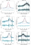 |
Fig. 1. Gaussian fits to the Hα and Hβ lines of the lensed systems. The red line is the best fit, the black lines are the different components of each region (emission and absorption), the green line is the Fe template, and the blue line is the continuum fit. The 1-sigma errors are shown by the blue regions, and the model residuals are shown below each spectrum. |
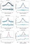 |
Fig. 1. continued. |
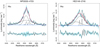 |
Fig. 1. continued. |
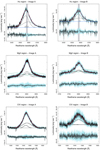 |
Fig. 2. Gaussian fits to the A and B image BELs of QJ0158-4325. The red line is the best fit, the black lines are the different components of each region (emission and absorption), the green line is the Fe template, and the blue line is the continuum fit. The 1-σ errors are shown by the blue regions, and the model residuals are shown below each spectrum. |
3.2. Luminosity measurements
We followed Assef et al. (2011) and estimated the monochromatic luminosity of each quasar using the broadband SED of the brightest image (A) and the fluxes from CASTLES and other sources in the literature (see Table A.1). If we obtained a useful spectrum of the fainter image, we also modeled its SED. This method was preferred over using the continuum obtained from the spectra due to several factors affecting the LUCIFER and MMIRS data (e.g., low S/N (3–18), unresolved images in the slit, seeing conditions varying between the target and the standard star) and because of the chromatic microlensing detected in the continuum of the four systems observed with X-shooter and FORS2 (Melo et al., in prep.). To demagnify the fluxes, we used the magnification estimated from a lens model (Table 2). We chose photometric data that were obtained close in time to our observations to minimize differences in the amount of microlensing or a large intrinsic variation that coupled with the time delay could mimic chromatic microlensing. If light curves were available, we included the variability amplitude as part of the flux uncertainties. For instance, Giannini et al. (2017) demonstrated that HE0047−1756 varied by ∼0.2–0.3 mag over a five-year period, and WFI2033−4723 varies by 0.5 mag in four years. The system HE0435−1223 varied ∼0.4 mag (Ricci et al. 2011) and more recently, Bonvin et al. (2017) presented 13-yr light curves with a variability amplitude of ∼0.7 mag.
Magnification values used for demagnifying the flux and their references.
3.3. Uncertainties
We needed to consider multiple factors that could contribute to the uncertainties in MBH. For example, the BEL of one of the images could be microlensed (e.g., microlensing affecting the red wing of the Hα emission line in HE0435−1223, Braibant et al. 2014, and the blue wing of MgII for the same system in Fian et al. 2018a), leading to a larger FWHM. Melo et al. (2021) showed that even if we have a FWHM difference between the images of > 5 sigma, the impact on MBH is negligible compared with other sources of errors (see below for a specific example).
Another contribution to the uncertainties is the blending of the images in some of the MMIRS spectra. To see how much this could affect the MBH, we compared the FWHM we found from fitting the blended image A+B spectrum of LBQS1333+0113 to the separate spectra of the two images (see Fig. 6). For Hα the FWHM of the combined spectrum is 4750 ± 110 km s−1 compared to 4610 ± 70 km s−1 for image A and 4755 ± 24 km s−1 for image B. These differences translate to estimated masses of log10(MBH/M⊙) = 9.16 ± 0.59, 9.13 ± 0.54, and 9.16 ± 0.48, which are much smaller than the other sources of error and thus unimportant for the BH mass estimate. A similar result is obtained for the MgII line.
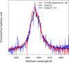 |
Fig. 6. Combined spectra of images A+B (red spectra), compared to image A (black spectra) and image B (blue spectra) for the system LBQS1333+0113. We subtracted the continuum for the three spectra and multiplied image B by a factor of 3.4 for a clearer comparison. |
Another factor contributing to the error is the monochromatic luminosity uncertainty. This has several systematic uncertainties: the systematic errors of the instrument, the magnification of the image given by the lens model, the flux calibration and intrinsic variability. To account for the intrinsic AGN variability, we added the observed variability as a contribution to the error in the monochromatic luminosity (Sect. 3.2). Although the uncertainties in the luminosity are large, the MBH estimate scales as L1/2, making it less sensitive to these errors compared to the FWHM because the MBH ∝ FWHM2 is so much stronger.
4. Results
Using the FWHM from the models of the emission lines and the monochromatic luminosity obtained from the SEDs, we measured MBH following Eq. (2). The results are shown in Table 3 along with their respective errors. Two systems have previous Hα log10(MBH/M⊙) (Assef et al. 2011): HE1104−1805 (9.05 ± 0.23) and SDSS1138+0314 (8.22 ± 0.22), respectively. Our estimate for HE1104−1805 is in agreement given its error (8.87 ± 0.70), while for SDSS1138+0314 the result is 0.27 dex smaller (7.95 ± 0.50). The difference in this case is due to a combination of factors: (1) we obtain a smaller FWHM (2330 ± 138 km s−1 versus 4700 ± 200 km s−1), (2) a lower luminosity (log10(L5100) = 44.57 ± 0.31) versus log10(L5100) = 44.81, 3), (3) a low S/N (∼10 for the spectra of image A in this work versus ∼8 for presented in Assef et al. 2011).
Hα and Hβ mass estimates of the observed images.
These are the first MBH estimates obtained for the systems QJ0158−4325 (log10(MBH/M⊙) = 8.05 ± 0.58, 8.51 ± 0.25, and 8.32 ± 0.46 for CIV, MgII, and Hα, respectively), HE0512−3329 (log10(MBH/M⊙) = 8.14 ± 0.25), and WFI2026−4536 (log10(MBH/M⊙) = 8.28 ± 0.25 and 7.83 ± 0.35, for Hα and Hβ, respectively).
The systems HE0047−1756, HE0435−1223, SDSS0924+0219, SDSS1226−0006, LBQS1333+0113, Q1355−2257, and WFI2033−4723 have previous estimates of MBH, which were made using the MgII emission lines (Peng et al. 2006; Sluse et al. 2012; Ding et al. 2017b), and we compared these estimates to our Balmer lines estimates in Fig. 7. Lensed quasars that have one or both MBH estimates presented in this work are shown in color. In general, our estimates are well correlated after we apply the offset of Mejía-Restrepo et al. (2016; 0.16 dex for MBH measured with Hα, and 0.25 dex using MgII). The systems in which the MBH differ for both lines (FBQ0951+2635, B1422+231, and Q2237+030) were obtained by different authors using different methods (Assef et al. 2011; Sluse et al. 2012) and different epochs.
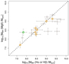 |
Fig. 7. Comparison between MBH estimates obtained from the Balmer lines and MgII emission lines. The new measurements are marked in orange (Hα emission line) and green (Hβ emission line). The systematic offset from Mejía-Restrepo et al. (2016) is applied. The dotted line shows where the masses are equal. |
The left panel of Fig. 8 shows the distribution in MBH and Lbol for our systems along with estimates from the literature for 34 lensed quasars (Peng et al. 2006; Greene et al. 2010; Assef et al. 2011; Sluse et al. 2012; Melo et al. 2021). Figure 8 (right) shows the distribution in luminosity and BH mass only considering the estimates from the Balmer lines. The Eddington ratios of the lensed quasars are typically close to ∼0.1, which agrees with the results from Shen et al. (2019) based on SE virial BH masses of quasars. Some of the systems have several values obtained from different emission lines. The intrinsic luminosity was converted to bolometric using Lbol = A × Lref, where A = (3.81, 5.15, 9.6) for Lref = (L1350, L3000 , L5100) from Sluse et al. (2012). MBH values obtained for non-lensed quasars using the SE method by Shen et al. (2019) are included as the contoured distribution for comparison. In general, the new MBH obtained from the Balmer lines span the same range of masses as the lensed and non-lensed AGNs (Fig. 8). In particular, we were able to obtain estimates for the lower-luminosity systems QJ0158−4325, SDSS0924+0219, HE0512−3329 and HE0047−1756 (from 1044 to 1046.5). The systems QJ0158−4325 and SDSS0924+0219 have the lowest luminosities (log10(Lref) < 44.60 L⊙), and the latter has the lowest MBH, log10(MBH/M⊙) = 7.43 ± 0.05 (this is the average of the Hα and Hβ estimates).
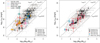 |
Fig. 8. Logarithmic MBH and bolometric luminosity. Left: for all available lensed quasars (Greene et al. 2010; Sluse et al. 2012; Assef et al. 2011; Peng et al. 2006; Melo et al. 2021) and for non-lensed quasars from Shen et al. (2011, 2019). The open triangles are the MBH estimates using Hα emission line, filled circles Hβ, open diamonds MgII, and open circles CIV. The measurements from this study are in color. Right: for just the Hα and Hβ emission lines. The red and blue points are our estimates. The dashed lines correspond to Eddington ratios of λ = 1, 0.1, and 0.01. |
We separately examined the three systems observed with X-shooter (QJ0158−4325, LBQS13333+0113, and Q1355−2257) because they have multiple MBH estimates using different emission lines. The SEDs were obtained independently for both images (A and B; see Table A.1), and the results show that the estimated magnification-corrected luminosity and MBH are in good agreement within the estimated errors.
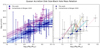 |
Fig. 9. Quasar accretion disk size-BH mass relation compared to that from Cornachione & Morgan (2020). Left: sample of lensed quasars rescaling our rs values to 2500 Å. A single power-law line is fitted to both samples. Right: same as the left panel but including only those sources common to both samples. The lines connect estimates for the same object. In some cases, the Cornachione & Morgan (2020) target is linked to two MBH estimates based on different emission lines (e.g., Hα and Hβ for SDSS1138+0314). |
In the case of LBQS1333+0113, we only used Hα and MgII because CIV line exhibits multiple absorption features and Hβ has low S/N (Melo et al., in prep). MgII and Hα are in good agreement with mean values of log10(MBH/M⊙) = 9.25 ± 0.51, and 9.01 ± 0.91, respectively. The FWHM of the Hα emission line observed with MMIRS is in agreement given its errors with that obtained with X-shooter. Sluse et al. (2012) obtained MBH from the MgII (log10(MBH/M⊙) = 9.19 ± 0.26), which agrees with our X-shooter result. Q1355−2257 exhibits a wide range of mass estimates depending on the emission line with mean values of log10(MBH/M⊙) = 8.20 ± 0.71, 9.12 ± 0.35 and 8.77 ± 0.88 for CIV, MgII, and Hα, respectively (green color in Fig. 8). The MgII measurement from Sluse et al. (2012) (log10(MBH/M⊙) = 9.04 ± 0.34) agrees with our estimate using the same line. As in the previous case, the CIV emission line for QJ0158−4325 is not consistent with the other estimates. The mean values for MgII and Hα are log10(MBH/M⊙) = 8.51 ± 0.27 and log10(MBH/M⊙) = 8.32 ± 0.52, respectively.
We were also able to estimate the unlensed size of the quasar accretion disk, rs (Eq. (3) of Mosquera & Kochanek 2011) using our MBH estimates and assuming a thin disk model (Shakura & Sunyaev 1973). The details of the parameters used are in Melo et al. (2021) and the size estimates are shown in Table 3. SDSS0924+0219 has the smallest accretion disk size (mean value between Hα and Hβ emission line of rs = 1014.78 ± 2.62 cm, an error in dex of 5.99. These spectra had very low signal-to-noise (∼5.9 and ∼3.9 in Hα and Hβ lines, respectively). The mean value for the systems QJ0158−4325, SDSS1226−0006, LBQS1333+0113 and Q1355−2257 (all emission lines from both images excluding CIV are 1015.28 ± 1.28 cm, 1015.33 ± 1.18 cm 1015.76 ± 0.89 cm and 1015.65 ± 1.13 cm, respectively.
Our rs estimates can be compared to the accretion disk sizes derived from microlensing using multi-epoch light curves (Cornachione & Morgan 2020, see our Fig. 9). We rescaled our rs to 2500 Å, the wavelength used by Cornachione & Morgan (2020), by assuming the relation rs ∝ λ4/3. While our uncertainties are larger, our results qualitatively agree with the conclusion of Cornachione & Morgan (2020), that microlensing radii are larger (∼0.5 dex) than expected from thin disk theory. In the right panel of Fig. 9 we show the MBH for those systems that are in both samples (seven). The BH mass estimates of the two studies differ for the same sample of objects, with the estimates in Cornachione & Morgan (2020) being higher than ours (except for SDSS1138+0314 and the MgII based estimate for QJ0158−4325), albeit generally within the error bars. Since the BH masses in Cornachione & Morgan (2020) are also estimated using the SE method, the differences must come from the exact prescriptions used to estimate them. Figure 9 shows, however, that the differences in rs are not driven by the difference in the BH estimates.
5. Conclusions
We estimated MBH using the broad Balmer emission lines of 14 lensed quasars measured using four different spectrographs (LUCI, MMIRS, X-shooter, and FORS2). After reducing and extracting the spectra corresponding to each image, the FWHMs of the BELs were estimated using the standard deviation of the model line profile after subtracting the narrow line components. The monochromatic luminosities were estimated using the de-magnified SED of the brightest image, taking the variability (if any) into account in the uncertainty budget.
These are the first MBH estimates for the systems QJ0158−4325, HE0512−3329, and WFI2026−4536. We also calculated MBH using the MgII emission line for the systems QJ0158−4325, SDSS1226−0006, LBQS13333+0113, and Q1355−2257.
We compared the new MBH Balmer line to previous MgII MBH estimates for HE0047−1756, HE0435−1223, SDSS0924+0219, SDSS1226−0006, LBQS1333+0113, Q1355−2257, and WFI2033−4723. The mass estimates are well correlated, with the exception of three lensed quasars (FBQ0951+2635, B1422+231, and Q2237+030), whose Balmer masses were not derived here.
The new Balmer MBH span the same range of mass estimates as non-lensed quasars, with the systems QJ0158−4325, SDSS0924+0219, HE0512−3329, and HE0047−1756 having the lowest luminosities. Three systems observed with X-shooter (QJ0158−4325, LBQS13333+0113, and Q1355−2257) were analyzed in detail because they have multiple MBH estimates based off different emission lines. The masses of the lensed quasars imply low Eddington ratios (∼0.1), in agreement with the results of Shen et al. (2019) from SE BH masses of SDSS quasars. Our MBH estimations are also consistent with those obtained from microlensing by Cornachione & Morgan (2020).
A decade after the initial BH mass measurements for gravitational lens systems (Peng et al. 2006; Greene et al. 2010; Assef et al. 2011; Sluse et al. 2012), this work expands the sample from 14 to 23 mass estimates. The MBH measurements of lensed quasars based on the Balmer lines show a lower dispersion in MBH (RMS ∼ 0.45 dex) at fixed bolometric luminosity, which is also true of non-lensed quasars (Shen et al. 2019). Including the MgII estimates increases the dispersion (RMS ∼ 0.65 dex), confirming that the Balmer lines are more reliable. An even larger dispersion is observed when the MgII lens MBH estimates from the literature are included. The recent discovery of new gravitational lens systems (Lemon et al. 2023) will allow us to explore the low-luminosity region.
Gravitationally Lensed Quasar Database, GQL https://research.ast.cam.ac.uk/lensedquasars/index.html
Acknowledgments
We thank Kelly Denney for help with the experimental design of the LUCI and MMIRS observations. We thank Franz Bauer and Ezequiel Treister for carrying out the MMIRS observations. We thank Daniela Zúñiga Sacks for help with the reduction of the LUCI data. R.J.A. was supported by FONDECYT grant number 1231718 and by the ANID BASAL project FB210003. V.M. acknowledges support from ANID FONDECYT Regular grant number 1231418 and Centro de Astrofísica de Valparaíso. N.G. acknowledges support by ANID, Millennium Science Initiative Program – NCN19_171. This project has received funding from the European Research Council (ERC) under the European Union’s Horizon Europe research and innovation programme (ESCAPE, grant agreement No 101044152). The LBT is an international collaboration among institutions in the United States, Italy and Germany. LBT Corporation partners are: The University of Arizona on behalf of the Arizona university system; Istituto Nazionale di Astrofisica, Italy; LBT Beteiligungsgesellschaft, Germany, representing the Max-Planck Society, the Astrophysical Institute Potsdam, and Heidelberg University; The Ohio State University, and The Research Corporation, on behalf of The University of Notre Dame, University of Minnesota and University of Virginia.
References
- Antonucci, R. 1993, ARA&A, 31, 473 [Google Scholar]
- Assef, R. J., Kochanek, C. S., Brodwin, M., et al. 2010, ApJ, 713, 970 [NASA ADS] [CrossRef] [Google Scholar]
- Assef, R. J., Denney, K. D., Kochanek, C. S., et al. 2011, ApJ, 742, 93 [Google Scholar]
- Barth, A. J., Bennert, V. N., Canalizo, G., et al. 2015, ApJS, 217, 26 [NASA ADS] [CrossRef] [Google Scholar]
- Baskin, A., & Laor, A. 2005, MNRAS, 356, 1029 [NASA ADS] [CrossRef] [Google Scholar]
- Bate, N. F., Vernardos, G., O’Dowd, M. J., et al. 2018, MNRAS, 479, 4796 [NASA ADS] [CrossRef] [Google Scholar]
- Bentz, M. C., Peterson, B. M., Pogge, R. W., Vestergaard, M., & Onken, C. A. 2006, ApJ, 644, 133 [NASA ADS] [CrossRef] [Google Scholar]
- Bentz, M. C., Peterson, B. M., Netzer, H., Pogge, R. W., & Vestergaard, M. 2009, ApJ, 697, 160 [Google Scholar]
- Bhatiani, S., Dai, X., & Guerras, E. 2019, ApJ, 885, 77 [NASA ADS] [CrossRef] [Google Scholar]
- Bonvin, V., Courbin, F., Suyu, S. H., et al. 2017, MNRAS, 465, 4914 [NASA ADS] [CrossRef] [Google Scholar]
- Braibant, L., Hutsemékers, D., Sluse, D., Anguita, T., & García-Vergara, C. J. 2014, A&A, 565, L11 [NASA ADS] [CrossRef] [EDP Sciences] [Google Scholar]
- Bujarrabal, V., Guibert, J., & Balkowski, C. 1981, A&A, 104, 1 [NASA ADS] [Google Scholar]
- Chilingarian, I., Beletsky, Y., Moran, S., et al. 2015, PASP, 127, 406 [CrossRef] [Google Scholar]
- Coatman, L., Hewett, P. C., Banerji, M., & Richards, G. T. 2016, MNRAS, 461, 647 [NASA ADS] [CrossRef] [Google Scholar]
- Coatman, L., Hewett, P. C., Banerji, M., et al. 2017, MNRAS, 465, 2120 [Google Scholar]
- Collin, S., Kawaguchi, T., Peterson, B. M., & Vestergaard, M. 2006, A&A, 456, 75 [NASA ADS] [CrossRef] [EDP Sciences] [Google Scholar]
- Cornachione, M. A., & Morgan, C. W. 2020, ApJ, 895, 93 [Google Scholar]
- Croton, D. J., Springel, V., White, S. D. M., et al. 2006, MNRAS, 365, 11 [Google Scholar]
- Deeming, T. J. 1964, MNRAS, 127, 493 [NASA ADS] [Google Scholar]
- Di Matteo, T., Springel, V., & Hernquist, L. 2005, Nature, 433, 604 [NASA ADS] [CrossRef] [Google Scholar]
- Ding, X., Liao, K., Treu, T., et al. 2017a, MNRAS, 465, 4634 [NASA ADS] [CrossRef] [Google Scholar]
- Ding, X., Treu, T., Suyu, S. H., et al. 2017b, MNRAS, 472, 90 [NASA ADS] [CrossRef] [Google Scholar]
- Ding, X., Treu, T., Birrer, S., et al. 2021, MNRAS, 501, 269 [Google Scholar]
- Du, P., Lu, K.-X., Hu, C., et al. 2016, ApJ, 820, 27 [NASA ADS] [CrossRef] [Google Scholar]
- Eigenbrod, A., Courbin, F., Meylan, G., Vuissoz, C., & Magain, P. 2006, A&A, 451, 759 [NASA ADS] [CrossRef] [EDP Sciences] [Google Scholar]
- Falco, E. E., Kochanek, C. S., Lehár, J., et al. 2001, ASP Conf. Ser., 237, 25 [Google Scholar]
- Ferrarese, L., & Merritt, D. 2000, ApJ, 539, L9 [Google Scholar]
- Fian, C., Guerras, E., Mediavilla, E., et al. 2018a, ApJ, 859, 50 [Google Scholar]
- Fian, C., Mediavilla, E., Jiménez-Vicente, J., Muñoz, J. A., & Hanslmeier, A. 2018b, ApJ, 869, 132 [NASA ADS] [CrossRef] [Google Scholar]
- Francis, P. J., & Wills, B. J. 1999, ASP Conf. Ser., 162, 363 [Google Scholar]
- Freudling, W., Romaniello, M., Bramich, D. M., et al. 2013, A&A, 559, A96 [NASA ADS] [CrossRef] [EDP Sciences] [Google Scholar]
- Giannini, E., Schmidt, R. W., Wambsganss, J., et al. 2017, A&A, 597, A49 [NASA ADS] [CrossRef] [EDP Sciences] [Google Scholar]
- Greene, J. E., & Ho, L. C. 2005, ApJ, 630, 122 [NASA ADS] [CrossRef] [Google Scholar]
- Greene, J. E., Peng, C. Y., & Ludwig, R. R. 2010, ApJ, 709, 937 [Google Scholar]
- Grier, C. J., Trump, J. R., Shen, Y., et al. 2017, ApJ, 851, 21 [NASA ADS] [CrossRef] [Google Scholar]
- Grier, C. J., Shen, Y., Horne, K., et al. 2019, ApJ, 887, 38 [NASA ADS] [CrossRef] [Google Scholar]
- Guerras, E., Dai, X., & Mediavilla, E. 2020, ApJ, 896, 111 [NASA ADS] [CrossRef] [Google Scholar]
- Hopkins, P. F., Hernquist, L., Cox, T. J., & Kereš, D. 2008, ApJS, 175, 356 [Google Scholar]
- Hutsemékers, D., & Sluse, D. 2021, A&A, 654, A155 [NASA ADS] [CrossRef] [EDP Sciences] [Google Scholar]
- Inada, N., Becker, R. H., Burles, S., et al. 2003, AJ, 126, 666 [NASA ADS] [CrossRef] [Google Scholar]
- Inada, N., Oguri, M., Becker, R. H., et al. 2008, AJ, 135, 496 [NASA ADS] [CrossRef] [Google Scholar]
- Kaspi, S., Smith, P. S., Netzer, H., et al. 2000, ApJ, 533, 631 [Google Scholar]
- Kaspi, S., Maoz, D., Netzer, H., et al. 2005, ApJ, 629, 61 [Google Scholar]
- Kausch, W., Noll, S., Smette, A., et al. 2015, A&A, 576, A78 [NASA ADS] [CrossRef] [EDP Sciences] [Google Scholar]
- Kochanek, C. S. 2004, ApJ, 605, 58 [Google Scholar]
- Kormendy, J., & Ho, L. C. 2013, ARA&A, 51, 511 [Google Scholar]
- Kormendy, J., & Richstone, D. 1995, ARA&A, 33, 581 [Google Scholar]
- Lemon, C., Anguita, T., Auger-Williams, M. W., et al. 2023, MNRAS, 520, 3305 [NASA ADS] [CrossRef] [Google Scholar]
- Lira, P., Kaspi, S., Netzer, H., et al. 2018, ApJ, 865, 56 [NASA ADS] [CrossRef] [Google Scholar]
- Malik, U., Sharp, R., Penton, A., et al. 2023, MNRAS, 520, 2009 [NASA ADS] [CrossRef] [Google Scholar]
- Marconi, A., & Hunt, L. K. 2003, ApJ, 589, L21 [Google Scholar]
- Marziani, P., Sulentic, J. W., Plauchu-Frayn, I., & del Olmo, A. 2013, A&A, 555, A89 [NASA ADS] [CrossRef] [EDP Sciences] [Google Scholar]
- McGill, K. L., Woo, J.-H., Treu, T., & Malkan, M. A. 2008, ApJ, 673, 703 [NASA ADS] [CrossRef] [Google Scholar]
- McLeod, B., Fabricant, D., Nystrom, G., et al. 2012, PASP, 124, 1318 [NASA ADS] [CrossRef] [Google Scholar]
- McLure, R. J., & Dunlop, J. S. 2004, MNRAS, 352, 1390 [NASA ADS] [CrossRef] [Google Scholar]
- McLure, R. J., & Jarvis, M. J. 2002, MNRAS, 337, 109 [Google Scholar]
- Mediavilla, E., & Jiménez-Vicente, J. 2021, ApJ, 914, 112 [NASA ADS] [CrossRef] [Google Scholar]
- Mediavilla, E., Muñoz, J. A., Falco, E., et al. 2009, ApJ, 706, 1451 [NASA ADS] [CrossRef] [Google Scholar]
- Mediavilla, E., Jiménez-vicente, J., Mejía-restrepo, J., et al. 2020, ApJ, 895, 111 [NASA ADS] [CrossRef] [Google Scholar]
- Mejía-Restrepo, J. E., Trakhtenbrot, B., Lira, P., Netzer, H., & Capellupo, D. M. 2016, MNRAS, 460, 187 [CrossRef] [Google Scholar]
- Mejía-Restrepo, J. E., Trakhtenbrot, B., Lira, P., & Netzer, H. 2018, MNRAS, 478, 1929 [CrossRef] [Google Scholar]
- Melo, A., Motta, V., Godoy, N., et al. 2021, A&A, 656, A108 [NASA ADS] [CrossRef] [EDP Sciences] [Google Scholar]
- Morgan, N. D., Dressler, A., Maza, J., Schechter, P. L., & Winn, J. N. 1999, AJ, 118, 1444 [NASA ADS] [CrossRef] [Google Scholar]
- Morgan, N. D., Gregg, M. D., Wisotzki, L., et al. 2003, AJ, 126, 696 [NASA ADS] [CrossRef] [Google Scholar]
- Morgan, N. D., Caldwell, J. A. R., Schechter, P. L., et al. 2004, AJ, 127, 2617 [CrossRef] [Google Scholar]
- Morgan, C. W., Kochanek, C. S., Morgan, N. D., & Falco, E. E. 2010, ApJ, 712, 1129 [Google Scholar]
- Mosquera, A. M., & Kochanek, C. S. 2011, ApJ, 738, 96 [Google Scholar]
- Muñoz, J. A., Mediavilla, E., Kochanek, C. S., Falco, E. E., & Mosquera, A. M. 2011, ApJ, 742, 67 [CrossRef] [Google Scholar]
- Netzer, H., & Peterson, B. M. 1997, Astrophys. Space Sci. Lib., 218, 85 [CrossRef] [Google Scholar]
- Netzer, H., & Trakhtenbrot, B. 2007, ApJ, 654, 754 [CrossRef] [Google Scholar]
- Oguri, M., Inada, N., Castander, F. J., et al. 2004, PASJ, 56, 399 [NASA ADS] [Google Scholar]
- Park, D., Woo, J.-H., Denney, K. D., & Shin, J. 2013, ApJ, 770, 87 [NASA ADS] [CrossRef] [Google Scholar]
- Park, D., Woo, J.-H., Bennert, V. N., et al. 2015, ApJ, 799, 164 [NASA ADS] [CrossRef] [Google Scholar]
- Peng, C. Y., Impey, C. D., Rix, H.-W., et al. 2006, ApJ, 649, 616 [Google Scholar]
- Peterson, B. M. 1993, PASP, 105, 247 [NASA ADS] [CrossRef] [Google Scholar]
- Peterson, B. M. 2014, Space. Sci. Rev., 183, 253 [NASA ADS] [CrossRef] [Google Scholar]
- Peterson, B. M., Ferrarese, L., Gilbert, K. M., et al. 2004, ApJ, 613, 682 [Google Scholar]
- Poindexter, S., Morgan, N., Kochanek, C. S., & Falco, E. E. 2007, ApJ, 660, 146 [NASA ADS] [CrossRef] [Google Scholar]
- Ricci, D., Poels, J., Elyiv, A., et al. 2011, A&A, 528, A42 [NASA ADS] [CrossRef] [EDP Sciences] [Google Scholar]
- Rojas, K., Motta, V., Mediavilla, E., et al. 2014, ApJ, 797, 61 [Google Scholar]
- Rupprecht, G., & Böhnhardt, H. 2000, FORS1+ 2 User Manual V1. 4, Tech. rep., VLT-MAN-ESO-13100-1543 [Google Scholar]
- Seifert, W., Appenzeller, I., Baumeister, H., et al. 2003, Proc. SPIE, 4841, 962 [NASA ADS] [CrossRef] [Google Scholar]
- Shakura, N. I., & Sunyaev, R. A. 1973, A&A, 500, 33 [NASA ADS] [Google Scholar]
- Shen, Y. 2013, Bull. Astron. Soc. India, 41, 61 [NASA ADS] [Google Scholar]
- Shen, Y., & Liu, X. 2012, ApJ, 753, 125 [NASA ADS] [CrossRef] [Google Scholar]
- Shen, Y., Greene, J. E., Strauss, M. A., Richards, G. T., & Schneider, D. P. 2008, ApJ, 680, 169 [Google Scholar]
- Shen, Y., Richards, G. T., Strauss, M. A., et al. 2011, ApJS, 194, 45 [Google Scholar]
- Shen, Y., Grier, C. J., Horne, K., et al. 2019, ApJ, 883, L14 [NASA ADS] [CrossRef] [Google Scholar]
- Shen, Y., Grier, C. J., Horne, K., et al. 2023, ArXiv e-prints [arXiv:2305.01014] [Google Scholar]
- Sluse, D., Hutsemékers, D., Courbin, F., Meylan, G., & Wambsganss, J. 2012, A&A, 544, A62 [NASA ADS] [CrossRef] [EDP Sciences] [Google Scholar]
- Smette, A., Sana, H., Noll, S., et al. 2015, A&A, 576, A77 [NASA ADS] [CrossRef] [EDP Sciences] [Google Scholar]
- Tremaine, S., Gebhardt, K., Bender, R., et al. 2002, ApJ, 574, 740 [NASA ADS] [CrossRef] [Google Scholar]
- Urry, C. M., & Padovani, P. 1995, PASP, 107, 803 [NASA ADS] [CrossRef] [Google Scholar]
- Vacca, W. D., Cushing, M. C., & Rayner, J. T. 2003, PASP, 115, 389 [NASA ADS] [CrossRef] [Google Scholar]
- Vernet, J., Dekker, H., D’Odorico, S., et al. 2011, A&A, 536, A105 [NASA ADS] [CrossRef] [EDP Sciences] [Google Scholar]
- Vestergaard, M. 2002, ApJ, 571, 733 [NASA ADS] [CrossRef] [Google Scholar]
- Vestergaard, M. 2004, ApJ, 601, 676 [CrossRef] [Google Scholar]
- Vestergaard, M., & Peterson, B. M. 2006, ApJ, 641, 689 [Google Scholar]
- Wandel, A., Peterson, B. M., & Malkan, M. A. 1999, ApJ, 526, 579 [NASA ADS] [CrossRef] [Google Scholar]
- Wang, J.-G., Dong, X.-B., Wang, T.-G., et al. 2009, ApJ, 707, 1334 [CrossRef] [Google Scholar]
- Wisotzki, L., Schechter, P. L., Bradt, H. V., Heinmüller, J., & Reimers, D. 2002, A&A, 395, 17 [NASA ADS] [CrossRef] [EDP Sciences] [Google Scholar]
- Woo, J.-H., Yoon, Y., Park, S., Park, D., & Kim, S. C. 2015, ApJ, 801, 38 [NASA ADS] [CrossRef] [Google Scholar]
- Woo, J.-H., Le, H. A. N., Karouzos, M., et al. 2018, ApJ, 859, 138 [NASA ADS] [CrossRef] [Google Scholar]
- Xiao, T., Barth, A. J., Greene, J. E., et al. 2011, ApJ, 739, 28 [NASA ADS] [CrossRef] [Google Scholar]
- Yu, Z., Martini, P., Penton, A., et al. 2023, MNRAS, 522, 4132 [NASA ADS] [CrossRef] [Google Scholar]
- Zu, Y., Kochanek, C. S., & Peterson, B. M. 2011, ApJ, 735, 80 [NASA ADS] [CrossRef] [Google Scholar]
- Zubovas, K., & King, A. R. 2019, Gen. Rel. Grav., 51, 65 [NASA ADS] [CrossRef] [Google Scholar]
Appendix A: Table of magnitudes
Magnitudes for images A and B (for five lensed quasars: QJ0158−4325, SDSS1226−0006, LBQS1333−0113, and Q1355−2257) of each system used for constructing the SED.
All Tables
Magnitudes for images A and B (for five lensed quasars: QJ0158−4325, SDSS1226−0006, LBQS1333−0113, and Q1355−2257) of each system used for constructing the SED.
All Figures
|
Fig. 1. Gaussian fits to the Hα and Hβ lines of the lensed systems. The red line is the best fit, the black lines are the different components of each region (emission and absorption), the green line is the Fe template, and the blue line is the continuum fit. The 1-sigma errors are shown by the blue regions, and the model residuals are shown below each spectrum. |
| In the text | |
|
Fig. 1. continued. |
| In the text | |
|
Fig. 1. continued. |
| In the text | |
|
Fig. 2. Gaussian fits to the A and B image BELs of QJ0158-4325. The red line is the best fit, the black lines are the different components of each region (emission and absorption), the green line is the Fe template, and the blue line is the continuum fit. The 1-σ errors are shown by the blue regions, and the model residuals are shown below each spectrum. |
| In the text | |
 |
Fig. 3. Same as Fig. 2 but for SDSS1226−0006. |
| In the text | |
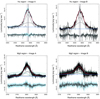 |
Fig. 4. Same as Fig. 2 but for LBQS1333+0113. |
| In the text | |
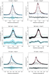 |
Fig. 5. Same as Fig. 2 but for Q1355−2257. |
| In the text | |
|
Fig. 6. Combined spectra of images A+B (red spectra), compared to image A (black spectra) and image B (blue spectra) for the system LBQS1333+0113. We subtracted the continuum for the three spectra and multiplied image B by a factor of 3.4 for a clearer comparison. |
| In the text | |
|
Fig. 7. Comparison between MBH estimates obtained from the Balmer lines and MgII emission lines. The new measurements are marked in orange (Hα emission line) and green (Hβ emission line). The systematic offset from Mejía-Restrepo et al. (2016) is applied. The dotted line shows where the masses are equal. |
| In the text | |
|
Fig. 8. Logarithmic MBH and bolometric luminosity. Left: for all available lensed quasars (Greene et al. 2010; Sluse et al. 2012; Assef et al. 2011; Peng et al. 2006; Melo et al. 2021) and for non-lensed quasars from Shen et al. (2011, 2019). The open triangles are the MBH estimates using Hα emission line, filled circles Hβ, open diamonds MgII, and open circles CIV. The measurements from this study are in color. Right: for just the Hα and Hβ emission lines. The red and blue points are our estimates. The dashed lines correspond to Eddington ratios of λ = 1, 0.1, and 0.01. |
| In the text | |
|
Fig. 9. Quasar accretion disk size-BH mass relation compared to that from Cornachione & Morgan (2020). Left: sample of lensed quasars rescaling our rs values to 2500 Å. A single power-law line is fitted to both samples. Right: same as the left panel but including only those sources common to both samples. The lines connect estimates for the same object. In some cases, the Cornachione & Morgan (2020) target is linked to two MBH estimates based on different emission lines (e.g., Hα and Hβ for SDSS1138+0314). |
| In the text | |
Current usage metrics show cumulative count of Article Views (full-text article views including HTML views, PDF and ePub downloads, according to the available data) and Abstracts Views on Vision4Press platform.
Data correspond to usage on the plateform after 2015. The current usage metrics is available 48-96 hours after online publication and is updated daily on week days.
Initial download of the metrics may take a while.