| Issue |
A&A
Volume 656, December 2021
|
|
|---|---|---|
| Article Number | A134 | |
| Number of page(s) | 13 | |
| Section | Astrophysical processes | |
| DOI | https://doi.org/10.1051/0004-6361/202141647 | |
| Published online | 15 December 2021 | |
Evolution patterns of the peak energy in the GRB prompt emission
1
School of Physics, Nanjing University, Nanjing 210023, PR China
2
Purple Mountain Observatory, Chinese Academy of Sciences, Nanjing 210023, PR China
e-mail: This email address is being protected from spambots. You need JavaScript enabled to view it.
3
School of Astronomy and Space Science, Nanjing University, Nanjing 210023, PR China
4
Key Laboratory of Modern Astronomy and Astrophysics (Nanjing University), Ministry of Education, Nanjing 210023, PR China
Received:
27
June
2021
Accepted:
22
September
2021
Abstract
Context. The peak energy (Ep) exhibited during the prompt emission phase of gamma-ray bursts (GRBs) shows two different evolution patterns, namely hard-to-soft and intensity-tracking, of which the physical origin remains unknown. In addition to low-energy indices of GRB prompt spectra, the evolution patterns of Ep may be another crucial indicator with which to discriminate radiation mechanisms (e.g., synchrotron or photosphere) for GRBs.
Aims. We explore the parameter space to find conditions that could generate different evolution patterns in the peak energy in the framework of synchrotron radiation.
Methods. We have developed a code to calculate the synchrotron emission from a simplified shell numerically, considering: three cooling processes (synchrotron, synchrotron self-Compton (SSC), and adiabatic) of electrons, the effect of decaying magnetic field, the effect of the bulk acceleration of the emitting shell, and the effect of a variable source function that describes electrons accelerated in the emitting region.
Results. After exploring the parameter space of the GRB synchrotron scenario, we find that the intensity-tracking pattern of Ep could be achieved in two situations. One is that the cooling process of electrons is dominated by adiabatic cooling or SSC+adiabatic cooling at the same time. The other is that the emitting region is under acceleration in addition to the cooling process being dominated by SSC cooling. Otherwise, hard-to-soft patterns of Ep are normally expected. Moreover, a chromatic intensity-tracking pattern of Ep could be induced by the effect of a variable source function.
Key words: gamma rays: general / radiation mechanisms: non-thermal / relativistic processes
© ESO 2021
1. Introduction
Gamma-ray bursts (GRBs), the most energetic stellar explosions in the Universe, have been observed and studied for several decades. The prompt emission of GRBs typically lasts for less than one second to several minutes and consists of several spikes in the light curve, which is thought to come from the relativistic jet launched from the central compact remnant (Blandford & Znajek 1977; Eichler et al. 1989; Piran 2004; Kumar & Zhang 2015). There are still several fundamental questions surrounding GRBs that remain unsolved; for example, the composition of GRB jets, the radiation mechanism producing GRBs, and the distance of the emitting region from the central engine (Zhang 2018) are all unknown.
The spectrum of the prompt emission is often described by the so-called Band function empirically (Band et al. 1993). In addition to the Band component, evidence has shown that multiple spectral components exist in some GRBs, such as an additional power-law component (Abdo et al. 2009a; Ackermann et al. 2011) in the high-energy band and a thermal component (Ghirlanda et al. 2003; Ryde 2005; Ryde & Pe’er 2009; Ryde et al. 2010; Pe’er & Ryde 2011; Guiriec et al. 2011, 2013; Lazzati et al. 2013; Iyyani et al. 2015; Li 2019; Li et al. 2021). Both synchrotron radiation of electrons (e.g., Mészáros et al. 1994; Tavani 1996; Zhang & Yan 2011) and photospheric emission (e.g., Rees & Mészáros 2005; Pe’er et al. 2006; Ryde et al. 2011) have been proposed to explain the GRB prompt emission. However, which radiation mechanism is responsible for most GRB spectra is still hotly debated.
The Band function is characterized by three parameters, the low-energy and high-energy photon spectral indices (α and β) and the peak energy (Ep). The “synchrotron line of death problem” (Preece et al. 1998) involving the statistics of α has been proposed to be in contention with a synchrotron origin for GRBs, although this contention was later eased by detailed treatment of the cooling processes of electrons (Derishev et al. 2001; Daigne et al. 2011; Uhm & Zhang 2014; Zhao et al. 2014; Geng et al. 2018a). Meanwhile, some efforts have been made on revising the modeled method for observed spectra (Zheng et al. 2012; Oganesyan et al. 2017, 2018; Ravasio et al. 2018). It is shown that there is a low-energy break in the prompt spectrum of some long GRBs. The low-energy break is described by two power-law indices α1 and α2, which have distributions centered around −2/3 and −3/2, respectively, and agree with the predictions of the synchrotron model. Notably, this additional spectral break at low energies was also confirmed in some short GRBs through a systematic search (Ravasio et al. 2019). Moreover, Burgess et al. (2020) suggest that synchrotron spectra from electrons in evolving (fast-to-slow) cooling regimes are capable of fitting ∼95% of all time-resolved spectra of the brightest long GRBs observed by the gamma-ray burst monitor (GBM: 8 keV–40 MeV) on board the NASA Fermi Gamma-Ray Observatory by comparing the theoretical results with observed data directly.
Thus, α may not be a good indicator with which to justify the radiation mechanism (Burgess et al. 2015; Iyyani et al. 2015; Meng et al. 2018). It was found that there are two distinct evolution patterns for Ep, namely hard-to-soft (Norris et al. 1986) and intensity-tracking (Golenetskii et al. 1983; Bhat et al. 1994; Kargatis et al. 1994; Ford et al. 1995; Preece et al. 2000; Lu et al. 2010, 2012; Ghirlanda et al. 2011; Li et al. 2019, 2021). In addition, Hakkila & Preece (2011) show that all single-pulse GRBs could follow the hard-to-soft evolution pattern. Although Ep is also derived from the Band function, its evolution pattern with a burst may represent an intrinsic trend rather than an artificial effect like α. Revealing the enigma of these distinct patterns may provide vital clues for understanding the physical mechanism of the GRB prompt emission.
The evolution patterns of Ep were studied in different dissipation and radiative processes. Zhang & Yan (2011) proposed that the GRB prompt emission comes from the sudden discharge of magnetic energy through turbulent magnetic reconnection, in which a hard-to-soft evolution of Ep throughout a pulse is predicted. In a sophisticated quasi-thermal GRB photosphere scenario, an intensity-tracking pattern for Ep could be naturally produced but the hard-to-soft pattern requires contrived physical condition (Deng & Zhang 2014). Beniamini & Granot (2016) discussed the temporal and spectral properties of prompt emission from magnetic reconnection. These authors found that magnetic reconnections could account for the hard-to-soft pattern and the intensity-tracking pattern for different comoving Lorentz factors of the field lines. However, the evolution of the electron spectra was not incorporated into this latter work.
In prevailing synchrotron models, the prompt emission comes from a relativistic jet or outflow launched from the central compact object (e.g., Bromberg et al. 2018; Kathirgamaraju et al. 2019; Geng et al. 2019). For a baryon-dominated jet, internal shocks could efficiently dissipate the relative kinetic energy of colliding shells into relativistic electrons (Narayan 1992; Rees & Meszaros 1994; Piran 1999). If the jet is Poynting-flux-dominated, turbulent magnetic reconnections are expected to accelerate electrons in the jet (Drenkhahn & Spruit 2002; Lyutikov & Blandford 2003; Zhang & Yan 2011). Uhm et al. (2018) considered a simple physical scenario in which a thin relativistic spherical shell expands while emitting photons isotropically in the shell. Assuming that the shell is under bulk acceleration (Uhm & Zhang 2016; Jia et al. 2016) and that the photons emitted obey an ad hoc spectral function without specifying its physical origin, two evolution patterns of Ep could then be reproduced. However, robust conclusion can only be achieved if modeling of the energy spectrum of electrons is spontaneously included in the calculations. Here, we focus on the synchrotron scenario and numerically calculate the evolution of the electron distribution to test the self-consistency of a synchrotron origin for the Ep evolution.
In this study, we investigate the conditions that make the evolution patterns of Ep in the framework of synchrotron radiation. Three main cooling processes (i.e., adiabatic, synchrotron, and synchrotron self-Compton (SSC)) for electrons and the effect of a decaying magnetic field are coherently considered in the calculation of electron distributions (Geng et al. 2018a; Zhang et al. 2019). Also, other possible effects like the dynamics of the shell (Uhm & Zhang 2016; Li & Zhang 2021), and the evolving pre-description of accelerated electrons are included in our investigation. A brief description of our synchrotron scenario is given in Sect. 2. Our numerical results are presented in Sect. 3, which include three distinct physical effects (Sects. 3.1–3.3). To test the applicability of our results, two short GRBs, namely GRB 090227B and GRB 110529A, are modeled (Sect. 3.4). Moreover, as another possible way to distinguish different radiation mechanisms, the numerical results of the prompt optical emission are presented (Sect. 3.5). Finally, in Sect. 4, we summarize and discuss our results. Some relevant formulations are given in the appendix.
2. Physical scenario
Let us consider a relativistic jet moving from an initial radius of R0 with a bulk Lorentz factor of Γ and emitting electrons in it. We trace the evolution of the distribution of electrons and derive the observed synchrotron flux density Fνobs from these electrons. The electrons are injected into the comoving background magnetic field of B′ (the superscript prime ′ denotes the quantities in the comoving frame hereafter), and the evolution of electrons could be obtained by solving the continuity equation in the energy space. The detailed procedure can be found in Appendix D and the numerical method is the same as that in Geng et al. (2018a). The distribution of injected electrons is assumed to be a power law of  for
for  , where Q0 is related to the injection rate by
  1. The electron spectral index p in shock theories ranges from 2.3 to 2.8 (Kirk et al. 2000; Sironi & Spitkovsky 2009). Quite large values (p > 3) in some GRBs are obtained through synchrotron fitting to the GRB spectra, making it a challenge to standard simulations in shocks and magnetic reconnection (Oganesyan et al. 2019; Ronchi et al. 2020; Burgess et al. 2020). However, the high-energy part of the spectrum is rarely constrained because GBM data are missing in most cases. Also, the evolution of the low-energy electron distribution mainly depends on its cooling process rather than p when high-energy electrons are continuously injected. Here, an intermediate value p = 2.7 is commonly adopted in view of particle simulations and observations, and this has little influence on our conclusions. The temporal structure of a GRB pulse consists of a fast rise and a shallow decay. To mimic such a GRB pulse, the injection of electrons into the jet is ceased at a turn-off time toff.
The Lorentz factor of the electrons that radiate at the GRB spectral peak energy is roughly  ; we then have
 (1)
(1)
where h is the Planck constant, c is the speed of light, qe and me are the electron charge and mass respectively, and z is the redshift of the burst. Here, z = 1 is adopted unless stated otherwise. When the jet encounters the surrounding interstellar medium, its bulk Lorentz factor Γ will decrease. Meanwhile, in a rapidly expanding jet, the magnetic field strength B′ will decay with radius according to  , where R is the radius of the expanding shell. As the radial component of the magnetic field decreases more rapidly than the toroidal component, the magnetic field is soon toroidally dominated, which decreases as R−1 (Lyubarsky 2009). Therefore, q is always set to be 1 in the main text (Uhm & Zhang 2015; Geng et al. 2018b), while the effect of different q (e.g., Ronchini et al. 2021) on our results is further discussed in Appendix D. Hence, as a function of decreasing Γ and B′, a hard-to-soft evolution pattern for Ep is naturally expected according to Eq. (1). Nevertheless, the real situation is probably much more complicated. The jet may be under acceleration driven by radiative pressure or the magnetic pressure gradient. Moreover, the observed flux comes from an equal-arrival-time surface (EATS) rather than a point-like emission site (Fenimore et al. 1996; Dermer 2004; Huang et al. 2007; Geng et al. 2017), and Eq. (1) is invalid for an integrated spectrum. Furthermore,
  might vary with time due to detailed particle acceleration processes (e.g., Guo et al. 2014). Therefore, other evolution patterns of Ep are likely to arise in specific conditions.
3. Numerical calculations
Instead of assuming a detailed model, we try to derive some constraints on relevant parameters used in our calculations from observations. The pulse duration tobs can be estimated by the angular timescale of the emitting shell, that is,
 (2)
(2)
from which the corresponding Γ can be obtained when tobs and the initial emission radius R0 are given. On the other hand, the specific flux at Ep in the observer frame can be estimated as (Sari et al. 1998; Kumar & McMahon 2008)
 (3)
(3)
where Ne is the total (already corrected for 4π solid angle) number of electrons with  and DL is the luminosity distance of the burst. Taking typical values for a GRB pulse as Ep ≃ 1 MeV, δtobs ≃ 1 s, and Fνobs ≃ 1 mJy, we can obtain plausible values for different sets of parameters (Γ,
  ,
,  ,
,  , R0) from Eqs. (1)–(3). More details can be found in Appendix B. Detailed parameter values are listed in Table 1, from which we derive evolving Ep (corresponding to the peak point of νobsFνobs) from the observed spectrum integrated over the EATS for each specific time (Appendix D). The curvature effect on Ep and Fνobs is thus naturally incorporated.
Parameters of numerical calculations.
To explore the conditions that generate distinct evolution patterns of Ep, we show results by adding physical effects progressively in the following sections. A shell moving at a constant Lorenz factor with two different starting radii where the shell begins to emit photons is modeled in Sect. 3.1. Two typical dissipation radii for GRB prompt emissions, namely R0 = 1014 cm and 1015 cm, are considered. A shell moving at an accelerating Lorenz factor is assumed and calculated in Sect. 3.2. We further investigate the case where the parameter  is varying in Sect. 3.3. Moreover, two short GRBs are modeled, namely GRB 090227B and GRB 110529A (Sect. 3.4). Finally, the prompt optical emission is discussed in Sect. 3.5.
3.1. Constant Γ
Here, we first assume that the expanding shell is moving at a constant Lorentz factor of Γ. In this group of calculations, we perform seven calculations, which are named in the form of “CXRYΓZ” with the letter C denoting the fact that Γ is constant. Here ‘X’ is an integer ranging from 1 to 4, where the numbers represent the dominating electron cooling process, that is, synchrotron cooling, synchrotron self-Compton (SSC) cooling, adiabatic cooling, and simultaneous SSC+adiabatic cooling, respectively. Y presents the logarithmic index of the starting radius and Z shows the value of Γ. The corresponding results, including the evolution of the electron distribution ( ), the flux density (Fν), the spectral energy distribution (νFν), light curves, and the evolution of Ep for each case are exhibited in Fig. 1.
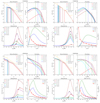 |
Fig. 1. Numerical results for seven cases in the first group shown in Table 1. The diagram of each case consists of four panels: the electron distribution |

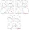 |
Fig. 1. continued. |
In the case of C1R14Γ240, the cooling process of electrons is forced to be dominated by synchrotron cooling by artificially ignoring SSC cooling. The electron distribution obeys the standard fast-cooling pattern ( ) in the early stage, and then its slope becomes flat because adiabatic cooling begins to dominate for low-energy electrons when B′ decreases. The corresponding synchrotron spectra and light curves show that Ep always decreases gradually during the rising and decaying stages of the pulse. Thus, a hard-to-soft pattern of Ep arises in this case. In C1R15Γ120, the cooling of electrons exactly traces the standard fast-cooling pattern for the entire duration. This is owing to the fact that the adiabatic cooling rate is inversely proportional to the radius of the shell (Uhm et al. 2012; Geng et al. 2014), and so synchrotron cooling dominates throughout. Meanwhile, Ep also exhibits a hard-to-soft evolution.
SSC cooling dominates in both C2R14Γ240 and C2R15Γ460, characterized by the fact that the slope of the low-energy electron spectrum approaches −1 (Bošnjak et al. 2009; Wang et al. 2009). Although the electron and the photon spectra are harder, Ep still appears to follow a hard-to-soft evolution in both cases. As shown in Fig. 1, for C3R14Γ1900, the dominance of adiabatic cooling leads to an even harder low-energy electron spectrum (Geng et al. 2018a). The evolution of Ep follows an intensity-tracking pattern. Electrons tend to gather in the low-energy scope due to the inefficient cooling rate. As a result, the slope of the low-energy electron spectrum becomes positive in one segment. Correspondingly, the peak intensity as well as the peak frequency in Fν spectrum changes slowly and slightly, which is different from the above cases. Equation (1) is now invalid and Ep is related to the integral of this segment of electrons. As an integral effect, the upwarp of the electron spectrum leads to a rightward shift of the peak point of the νFν spectrum. The electron spectrum of  would generate a flux density of
  . If the slope of the low-energy spectra exceeds zero, the index of the corresponding Fν spectra will be greater than 0.5. As a result, the peak point of the νFν spectrum will shift towards high frequencies.
Unlike C3R14Γ1900, a larger initial radius of the shell in C3R15Γ1900 results in a slower magnetic decay, and the cooling process is dominated by synchrotron cooling rather than adiabatic cooling. In this case, Ep exhibits a hard-to-soft evolution. If SSC cooling together with adiabatic cooling governs the cooling process, the electron spectrum will quickly harden. As a consequence, it also shows an intensity-tracking evolution for Ep. This is presented in the case of C4R14Γ460.
According to these results, hard-to-soft evolution for Ep is normally expected with constant Γ. The necessary condition for generation of the intensity-tracking pattern is that the slope of the low-energy electron spectra at the early stage must be harder than −1.0. This requires that electrons be dominated by adiabatic cooling or adiabatic+SSC cooling.
3.2. Increasing Γ
A bulk acceleration of Γ may lead to the increase in Ep according to Eq. (1). Both radiative pressure and the magnetic pressure gradient within the jet could be responsible for the acceleration of the jet (e.g., Piran et al. 1993; Drenkhahn 2002; Geng et al. 2021). We therefore consider that the Lorentz factor of the shell is increasing gradually (Uhm et al. 2018), that is,
 (4)
(4)
where R is the radius of the shell at some time. The acceleration index s ranges from one-third to one in different acceleration theories (Drenkhahn 2002; Komissarov et al. 2009). Three representative values, namely 0.35, 0.55, and 1.0, are taken in calculations. Similar to those in the previous section, we consider two possible initial radiation radiuses of the shell. This group of numerical results are presented in Fig. 2, which are named in the form of “ARYΓZ”. ‘A’ signifies that the shell is accelerating, Y is the logarithmic index of the starting radius, and Z is the initial Lorentz factor Γ0 of the shell.
In AR14Γ200, s is set to be 0.35 and the cooling process is dominated by SSC cooling. The low-energy electron spectrum gets hard within a very early period, while the Fν spectrum in the high-frequency domain does not change significantly over time. Ep exhibits an intensity-tracking pattern evolution, which is distinct from the case of C2R14Γ240. On the one hand, the increasing Γ leads to the rise in Ep analytically. On the other hand, we find that the EATS effect opposes the occurrence of the intensity-tracking pattern. The acceleration effect compels photons to gather at low latitudes of the EATS and weakens the EATS effect. Thus, C2R14Γ240 does not present an intensity-tracking pattern of Ep. In AR14Γ150, s is 0.55 and SSC cooling is also dominant. The slope of the low-energy electron spectrum tends to be −1 early and exceeds −1 at the late stage. The evolution curve of Ep also shows an intensity-tracking pattern. In AR14Γ80, s is 1.0. The electron distribution and the flux density are similar to those in AR14Γ150. Ep presents an intensity-tracking evolution again.
As for the case of AR15Γ230, s is 1.0, and a hard-to-soft evolution for Ep is shown, which is a natural result from the dominance of synchrotron cooling and the EATS effect. Owing to a larger initial radius, the photon energy density is reduced significantly meaning that it is hard for the SSC cooling to dominate the cooling process at an early time. As a result, the low-energy electron spectra follow the standard cooling except for the last stage. Moreover, the moving distance of the shell during δtobs is only the magnitude of R0, which implies a strong EATS effect on Fν.
In this section, the significance of SSC cooling and the bulk acceleration effect are discussed. SSC cooling alone is not able to produce an intensity-tracking pattern in Ep because the EATS effect impedes the formation of such a pattern. However, an accelerating shell working together with a dominant SSC cooling could generate an intensity-tracking pattern in Ep for a small initial radius of 1014 cm. For a larger initial radius of 1015 cm, only a hard-to-soft pattern can form, even for an accelerating shell, because of the absence of SSC cooling dominance.
3.3. A variable source function
The particle-in-cell simulations for relativistic magnetic reconnections indicate that the accelerated particle spectrum is evolving with time (e.g., Guo et al. 2014). Here, we take a variable source function into account. Specifically, a broken power-law profile of  (Uhm et al. 2018) is assumed,
 (5)
(5)
where Ra is the radius beyond which particle acceleration efficiency begins to decrease. In the real situation, the turnover time for particle acceleration efficiency is probably not identical to toff. Thus, Ra is set to be smaller than Roff which corresponds to toff. Similarly, four cases are included in this group of numerical results (see Table 1), and the corresponding figures are exhibited in Fig. 3. The cases are named in the form of “AGXRYΓZ”, where ‘G’ indicates that the evolution of  is taken into account, ‘X’ is an integer ranging from 1 to 2, denoting the bulk acceleration effect is considered or not, respectively. The meanings of Y and Z are the same as in Sect. 3.2.
In AG1R14Γ300, SSC cooling is dominant at the early stage and the slope of the low-energy electron spectra tends to −1, which is the same as the case of AG2R14Γ150. In AG1R14Γ300, we first consider the evolution of  only and ignore the bulk acceleration effect. AG1R14Γ300 presents a chromatic intensity-tracking pattern for Ep, which means that the peak time of Ep and the light curve are mismatched. When the bulk acceleration effect is also included in A2R14Γ150, a chromatic intensity-tracking is seen. This chromatic intensity-tracking pattern for Ep has not been seen in observations. Different from the above intensity-tracking patterns, the chromatic intensity-tracking pattern is induced by the effect of a variable source function which reflects the intrinsic particle acceleration. An intensity-tracking pattern is expected for Ep when Ra is set to be the same value as Roff. If this new pattern is confirmed from detailed data analyses in the future, this would evidence the varying
  from particle acceleration.
In results for AG1R15Γ250, owing to the large initial radius, synchrotron cooling simply dominates the whole cooling process and SSC cooling emerges at the last stage. Also, a large initial radius causes the EATS effect to strongly affect the observed flux density because of the little movement of the shell relative to the initial radius (also see Appendix B). Consequently, the role of the varying  is suppressed by the synchrotron cooling dominance and the EATS effect. It is therefore is understandable that Ep shows a hard-to-soft evolution pattern. On the other hand, for AG2R15Γ230, both the bulk acceleration effect and the varying
  are considered. The EATS effect is weakened so that Ep presents a chromatic intensity-tracking pattern again at the very early stage.
3.4. Application to GRB data
To test the applicability of our calculations, we performed theoretical modeling of two representative short GRBs, namely GRB 110529A (intensity-tracking) and GRB 090227B (hard-to-soft), respectively. The data used from Fermi-GBM2 were analyzed with the standard Bayesian approach and the time bin selection method to obtain the time-resolved spectra (see details in Li et al. 2019). Because of the huge computational cost of each calculation and the potentially strong degeneracy between the parameters, a strict fitting procedure with the Bayesian method was not carried out in the study presented here. Instead, we manually changed the physical parameters involved until a good match was seen visually between the numerical results and the data. The fitting parameters are listed in Table 2. As is shown in Fig. 4, it was possible to roughly reproduce the evolution of Ep and flux for these two GRBs.
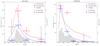 |
Fig. 4. Theoretical modeling of light curves and Ep evolutions for GRB 110529A and GRB 090227B. In each diagram, numerical results are shown with blue (for flux) and red (for Ep) lines, while the observational data are presented by blue (for flux) and red (for Ep) dots. The gray histogram shows the photon-count light curve in a scaled way. |
The fitting parameters.
In GRB 110529A, an accelerating shell is assumed and SSC cooling is dominant, leading to a rapid rise of the light curve and an intensity-tracking pattern in Ep. In GRB 090227B, the shell is moving at a constant Lorentz factor and the cooling process is dominated by synchrotron cooling, resulting in a hard-to-soft pattern in Ep. We note that there is a distinct sub-pulse every 0.1−0.15 s as shown in photon counts of GRB 090227B, which leads to the significant deviation of theoretical Ep from the observed one during this period.
3.5. The prompt optical emission
A review of the relevant literature indicates that we need more probes to distinguish possible radiation mechanisms in addition to the evolution patterns of Ep and the low-energy spectral indices. Therefore, in this section, we calculate the prompt optical emission of the above 15 distinct cases. The representative results are exhibited in Fig. 5, including C1R15Γ120, C2R15Γ460, and AR14Γ150.
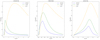 |
Fig. 5. Representative results of the prompt optical emission from three cases in Table 1. There are three light curves in different energy bands in the diagram of each case, including 2 eV, 1 keV, and 10 keV. |
As shown in Fig. 5, the flux of the prompt optical emission is higher than the prompt X-ray emission but within only one magnitude. A clear spectral lag and a shallower decay for the optical emission are present. The detection sensitivity of the Ground-based Wide Angle Camera (GWAC) and future Wide Field Survey Telescope (WFST) of China is roughly 15 and 20 apparent magnitudes in the R band within an exposure time of one second. Accordingly, prompt synchrotron optical emissions from a burst within ∼1 Gpc are detectable by GWAC (∼10 Gpc by WFST). Future observations of the prompt optical emission will help us to examine the synchrotron radiation scenarios.
4. Conclusions and discussion
In this article, we numerically trace the evolution of electrons and the corresponding synchrotron emissions in the framework of synchrotron radiation, to explore possible evolution patterns of Ep. We analyzed the effects of the bulk acceleration of the emitting shell, the varying  , and the EATS by performing groups of calculations. In addition, the prompt optical emission is calculated. Our conclusions can be summarized as follows:
1. For a shell moving at a constant Lorentz factor, the intensity-tracking pattern of Ep could emerge when electrons are dominated by adiabatic cooling or adiabatic+SSC cooling. For the case of pure dominance by adiabatic cooling, a bulk Lorentz factor Γ of > 1000 for the shell and a small emitting radius of R0 ≤ 1014 cm are required. Otherwise, a hard-to-soft pattern is normally expected.
2. For a shell under bulk acceleration, a dominant SSC cooling could generate an intensity-tracking pattern of Ep for a small initial radius of 1014 cm. However, for a larger initial radius of 1015 cm, only a hard-to-soft pattern is seen even for an accelerating shell, owing to the synchrotron cooling dominance and the EATS effect.
3. When the role of the intrinsic evolution of  is taken into account, a chromatic intensity-tracking for Ep may occur. Also, the rapid decay of B′ (q ≥ 1.5), accompanied by dominant adiabatic cooling, would generate an Ep that tracks chromatic intensity (Appendix D).
4. The flux density of the prompt optical emission is slightly higher than the prompt X-ray emission, and is detectable for bursts within ∼1 Gpc by current wide-field telescopes like GWAC, and ∼10 Gpc by the future WFST of China.
Recently, Ronchini et al. (2021) showed a relation between spectral index and flux by investigating the X-ray tails of bright GRB pulses, which is incompatible with the long-standing scenario that invokes the delayed arrival of photons from high-latitude parts of the jet. It is suggested that a dominating adiabatic cooling process, accompanied by the decay of the magnetic field, could explain this relation after testing several possible cooling mechanisms. The present study supports that adiabatic cooling could play a significant role in the GRB prompt phase.
These distinct evolution patterns, namely hard-to-soft, intensity-tracking, and chromatic intensity-tracking, reflect different physical processes in the GRB prompt emission. In general, the intensity-tracking pattern of Ep indicates that the bulk Lorentz factor is initially very large or is under acceleration, and the emitting radius should be relatively small. The evolution of  from the particle acceleration process could generate a chromatic intensity-tracking pattern. Further studies could help to test our conclusions.
Although the intensity-tracking pattern is found here for a single short pulse of the GRB, our results are applicable to a long-duration burst that consists of several pulses. Owing to the proportional relation observed between Fνobs and Ep in time-resolved pulses, it is naturally expected that a long-duration burst presents the same evolution pattern in Ep as the single pulse.
In the current work, the source function  is set the form of a power law, namely
  , which should be derived from detailed modeling of the particle acceleration process in our future works. On the other hand, we assume here that the shell is homogeneous in latitude and that its thickness can be ignored. Further considerations on the structure of the shell may be specified in the future.
In addition to studies on the evolution pattern of Ep within the synchrotron radiation scenarios, its interpretation within the framework of photosphere radiation is urgently encouraged. Also, better indicators (like Ep, the curvature of the spectrum, etc.) with which to identify the underlying radiation mechanism are now being discussed. For example, the characteristics of the low-energy band (i.e., less than 1 keV) for GRB prompt emissions may show distinct properties within different physical scenarios (Oganesyan et al. 2018; Toffano et al. 2021). Therefore, theoretical and observational efforts are encouraged in the investigation of the prompt optical emission.
 is the maximum Lorentz factor of electrons and is given by the approximation
  (Huang et al. 2000).
Acknowledgments
We appreciate the anonymous referee for constructive suggestions. We acknowledge the use of the public data from the Fermi data archives. We also would like to thank Xue-Feng Wu for the helpful discussion and Liang Li for providing the GRB data. This work is supported by National SKA Program of China No. 2020SKA0120300, by the National Natural Science Foundation of China (Grant Nos. 11903019, 11873030, 11833003, 12041306, U1938201, 11535005), and by the Strategic Priority Research Program of the Chinese Academy of Sciences (“multi-waveband Gravitational-Wave Universe”, Grant No. XDB23040000).
References
- Abdo, A. A., Ackermann, M., Ajello, M., et al. 2009a, ApJ, 706, L138 [NASA ADS] [CrossRef] [Google Scholar]
- Abdo, A. A., Ackermann, M., Arimoto, M., et al. 2009b, Science, 323, 1688 [NASA ADS] [CrossRef] [Google Scholar]
- Ackermann, M., Ajello, M., Asano, K., et al. 2011, ApJ, 729, 114 [CrossRef] [Google Scholar]
- Band, D., Matteson, J., Ford, L., et al. 1993, ApJ, 413, 281 [Google Scholar]
- Beniamini, P., & Granot, J. 2016, MNRAS, 459, 3635 [NASA ADS] [CrossRef] [Google Scholar]
- Bhat, P. N., Fishman, G. J., Meegan, C. A., et al. 1994, ApJ, 426, 604 [NASA ADS] [CrossRef] [Google Scholar]
- Blandford, R. D., & Znajek, R. L. 1977, MNRAS, 179, 433 [NASA ADS] [CrossRef] [Google Scholar]
- Blumenthal, G. R., & Gould, R. J. 1970, Rev. Mod. Phys., 42, 237 [Google Scholar]
- Bošnjak, Ž., Daigne, F., & Dubus, G. 2009, A&A, 498, 677 [NASA ADS] [CrossRef] [EDP Sciences] [Google Scholar]
- Bromberg, O., Tchekhovskoy, A., Gottlieb, O., Nakar, E., & Piran, T. 2018, MNRAS, 475, 2971 [NASA ADS] [CrossRef] [Google Scholar]
- Burgess, J. M., Ryde, F., & Yu, H.-F. 2015, MNRAS, 451, 1511 [Google Scholar]
- Burgess, J. M., Bégué, D., Greiner, J., et al. 2020, Nat. Astron., 4, 174 [Google Scholar]
- Daigne, F., Bošnjak, Ž., & Dubus, G. 2011, A&A, 526, A110 [NASA ADS] [CrossRef] [EDP Sciences] [Google Scholar]
- Deng, W., & Zhang, B. 2014, ApJ, 785, 112 [NASA ADS] [CrossRef] [Google Scholar]
- Derishev, E. V., Kocharovsky, V. V., & Kocharovsky, V. V. 2001, A&A, 372, 1071 [NASA ADS] [CrossRef] [EDP Sciences] [Google Scholar]
- Dermer, C. D. 2004, ApJ, 614, 284 [NASA ADS] [CrossRef] [Google Scholar]
- Drenkhahn, G. 2002, A&A, 387, 714 [NASA ADS] [CrossRef] [EDP Sciences] [Google Scholar]
- Drenkhahn, G., & Spruit, H. C. 2002, A&A, 391, 1141 [NASA ADS] [CrossRef] [EDP Sciences] [Google Scholar]
- Eichler, D., Livio, M., Piran, T., & Schramm, D. N. 1989, Nature, 340, 126 [NASA ADS] [CrossRef] [Google Scholar]
- Fenimore, E. E., Madras, C. D., & Nayakshin, S. 1996, ApJ, 473, 998 [NASA ADS] [CrossRef] [Google Scholar]
- Ford, L. A., Band, D. L., Matteson, J. L., et al. 1995, ApJ, 439, 307 [NASA ADS] [CrossRef] [Google Scholar]
- Geng, J. J., Wu, X. F., Li, L., Huang, Y. F., & Dai, Z. G. 2014, ApJ, 792, 31 [NASA ADS] [CrossRef] [Google Scholar]
- Geng, J. J., Wu, X. F., Huang, Y. F., Li, L., & Dai, Z. G. 2016, ApJ, 825, 107 [NASA ADS] [CrossRef] [Google Scholar]
- Geng, J.-J., Huang, Y.-F., & Dai, Z.-G. 2017, ApJ, 841, L15 [NASA ADS] [CrossRef] [Google Scholar]
- Geng, J.-J., Huang, Y.-F., Wu, X.-F., Zhang, B., & Zong, H.-S. 2018a, ApJS, 234, 3 [Google Scholar]
- Geng, J.-J., Huang, Y.-F., Wu, X.-F., Song, L.-M., & Zong, H.-S. 2018b, ApJ, 862, 115 [NASA ADS] [CrossRef] [Google Scholar]
- Geng, J.-J., Zhang, B., Kölligan, A., Kuiper, R., & Huang, Y.-F. 2019, ApJ, 877, L40 [CrossRef] [Google Scholar]
- Geng, J., Li, B., & Huang, Y. 2021, The Innovation, 2, 100152 [NASA ADS] [CrossRef] [Google Scholar]
- Ghirlanda, G., Celotti, A., & Ghisellini, G. 2003, A&A, 406, 879 [NASA ADS] [CrossRef] [EDP Sciences] [Google Scholar]
- Ghirlanda, G., Ghisellini, G., Nava, L., & Burlon, D. 2011, MNRAS, 410, L47 [NASA ADS] [CrossRef] [Google Scholar]
- Golenetskii, S. V., Mazets, E. P., Aptekar, R. L., & Ilinskii, V. N. 1983, Nature, 306, 451 [NASA ADS] [CrossRef] [Google Scholar]
- Guiriec, S., Connaughton, V., Briggs, M. S., et al. 2011, ApJ, 727, L33 [NASA ADS] [CrossRef] [Google Scholar]
- Guiriec, S., Daigne, F., Hascoët, R., et al. 2013, ApJ, 770, 32 [NASA ADS] [CrossRef] [Google Scholar]
- Guo, F., Li, H., Daughton, W., & Liu, Y.-H. 2014, Phys. Rev. Lett., 113, 155005 [Google Scholar]
- Hakkila, J., & Preece, R. D. 2011, ApJ, 740, 104 [NASA ADS] [CrossRef] [Google Scholar]
- Huang, Y. F., Gou, L. J., Dai, Z. G., & Lu, T. 2000, ApJ, 543, 90 [NASA ADS] [CrossRef] [Google Scholar]
- Huang, Y.-F., Lu, Y., Wong, A. Y. L., & Cheng, K. S. 2007, Chin. J. Astron. Astrophys., 7, 397 [CrossRef] [Google Scholar]
- Iyyani, S., Ryde, F., Ahlgren, B., et al. 2015, MNRAS, 450, 1651 [NASA ADS] [CrossRef] [Google Scholar]
- Jia, L.-W., Uhm, Z. L., & Zhang, B. 2016, ApJS, 225, 17 [CrossRef] [Google Scholar]
- Kargatis, V. E., Liang, E. P., Hurley, K. C., et al. 1994, ApJ, 422, 260 [NASA ADS] [CrossRef] [Google Scholar]
- Kathirgamaraju, A., Tchekhovskoy, A., Giannios, D., & Barniol Duran, R. 2019, MNRAS, 484, L98 [CrossRef] [Google Scholar]
- Kirk, J. G., Guthmann, A. W., Gallant, Y. A., & Achterberg, A. 2000, ApJ, 542, 235 [Google Scholar]
- Komissarov, S. S., Vlahakis, N., Königl, A., & Barkov, M. V. 2009, MNRAS, 394, 1182 [NASA ADS] [CrossRef] [Google Scholar]
- Kumar, P., & McMahon, E. 2008, MNRAS, 384, 33 [NASA ADS] [CrossRef] [Google Scholar]
- Kumar, P., & Zhang, B. 2015, Phys. Rep., 561, 1 [Google Scholar]
- Lazzati, D., Morsony, B. J., Margutti, R., & Begelman, M. C. 2013, ApJ, 765, 103 [NASA ADS] [CrossRef] [Google Scholar]
- Li, L. 2019, ApJS, 245, 7 [NASA ADS] [CrossRef] [Google Scholar]
- Li, L., & Zhang, B. 2021, ApJS, 253, 43 [NASA ADS] [CrossRef] [Google Scholar]
- Li, L., Geng, J.-J., Meng, Y.-Z., et al. 2019, ApJ, 884, 109 [CrossRef] [Google Scholar]
- Li, L., Ryde, F., Pe’er, A., Yu, H.-F., & Acuner, Z. 2021, ApJS, 254, 35 [NASA ADS] [CrossRef] [Google Scholar]
- Lithwick, Y., & Sari, R. 2001, ApJ, 555, 540 [NASA ADS] [CrossRef] [Google Scholar]
- Longair, M. S. 2011, High Energy Astrophysics (Cambridge: Cambridge University Press) [Google Scholar]
- Lu, R. J., Hou, S. J., & Liang, E.-W. 2010, ApJ, 720, 1146 [NASA ADS] [CrossRef] [Google Scholar]
- Lu, R.-J., Wei, J.-J., Liang, E.-W., et al. 2012, ApJ, 756, 112 [Google Scholar]
- Lyubarsky, Y. 2009, ApJ, 698, 1570 [NASA ADS] [CrossRef] [Google Scholar]
- Lyutikov, M., & Blandford, R. 2003, ArXiv e-prints [arXiv:astro-ph/0312347] [Google Scholar]
- Meng, Y.-Z., Geng, J.-J., Zhang, B.-B., et al. 2018, ApJ, 860, 72 [NASA ADS] [CrossRef] [Google Scholar]
- Mészáros, P., & Rees, M. J. 1999, MNRAS, 306, L39 [CrossRef] [Google Scholar]
- Mészáros, P., & Rees, M. J. 2000, ApJ, 530, 292 [Google Scholar]
- Mészáros, P., Rees, M. J., & Papathanassiou, H. 1994, ApJ, 432, 181 [CrossRef] [Google Scholar]
- Narayan, R. 1992, ApJ, 394, 261 [NASA ADS] [CrossRef] [Google Scholar]
- Norris, J. P., Share, G. H., Messina, D. C., et al. 1986, ApJ, 301, 213 [NASA ADS] [CrossRef] [Google Scholar]
- Oganesyan, G., Nava, L., Ghirlanda, G., & Celotti, A. 2017, ApJ, 846, 137 [Google Scholar]
- Oganesyan, G., Nava, L., Ghirlanda, G., & Celotti, A. 2018, A&A, 616, A138 [NASA ADS] [CrossRef] [EDP Sciences] [Google Scholar]
- Oganesyan, G., Nava, L., Ghirlanda, G., Melandri, A., & Celotti, A. 2019, A&A, 628, A59 [NASA ADS] [CrossRef] [EDP Sciences] [Google Scholar]
- Pe’er, A., & Ryde, F. 2011, ApJ, 732, 49 [CrossRef] [Google Scholar]
- Pe’er, A., Mészáros, P., & Rees, M. J. 2006, ApJ, 642, 995 [CrossRef] [Google Scholar]
- Piran, T. 1999, Nucl. Phys. B Proc. Suppl., 70, 431 [CrossRef] [Google Scholar]
- Piran, T. 2004, Rev. Mod. Phys., 76, 1143 [Google Scholar]
- Piran, T., Shemi, A., & Narayan, R. 1993, MNRAS, 263, 861 [NASA ADS] [Google Scholar]
- Preece, R. D., Briggs, M. S., Mallozzi, R. S., et al. 1998, ApJ, 506, L23 [Google Scholar]
- Preece, R. D., Briggs, M. S., Mallozzi, R. S., et al. 2000, ApJS, 126, 19 [Google Scholar]
- Ravasio, M. E., Oganesyan, G., Ghirlanda, G., et al. 2018, A&A, 613, A16 [NASA ADS] [CrossRef] [EDP Sciences] [Google Scholar]
- Ravasio, M. E., Ghirlanda, G., Nava, L., & Ghisellini, G. 2019, A&A, 625, A60 [NASA ADS] [CrossRef] [EDP Sciences] [Google Scholar]
- Rees, M. J., & Meszaros, P. 1994, ApJ, 430, L93 [Google Scholar]
- Rees, M. J., & Mészáros, P. 2005, ApJ, 628, 847 [NASA ADS] [CrossRef] [Google Scholar]
- Ronchi, M., Fumagalli, F., Ravasio, M. E., et al. 2020, A&A, 636, A55 [NASA ADS] [CrossRef] [EDP Sciences] [Google Scholar]
- Ronchini, S., Oganesyan, G., Branchesi, M., et al. 2021, Nat. Commun., 12, 4040 [NASA ADS] [CrossRef] [Google Scholar]
- Rybicki, G. B., & Lightman, A. P. 1986, Radiative Processes in Astrophysics (Weinheim: Wiley-VCH) [Google Scholar]
- Ryde, F. 2005, ApJ, 625, L95 [NASA ADS] [CrossRef] [Google Scholar]
- Ryde, F., & Pe’er, A. 2009, ApJ, 702, 1211 [NASA ADS] [CrossRef] [Google Scholar]
- Ryde, F., Axelsson, M., Zhang, B. B., et al. 2010, ApJ, 709, L172 [Google Scholar]
- Ryde, F., Pe’er, A., Nymark, T., et al. 2011, MNRAS, 415, 3693 [NASA ADS] [CrossRef] [Google Scholar]
- Sari, R., & Esin, A. A. 2001, ApJ, 548, 787 [NASA ADS] [CrossRef] [Google Scholar]
- Sari, R., Piran, T., & Narayan, R. 1998, ApJ, 497, L17 [Google Scholar]
- Sironi, L., & Spitkovsky, A. 2009, ApJ, 698, 1523 [NASA ADS] [CrossRef] [Google Scholar]
- Sironi, L., Spitkovsky, A., & Arons, J. 2013, ApJ, 771, 54 [Google Scholar]
- Spruit, H. C., Daigne, F., & Drenkhahn, G. 2001, A&A, 369, 694 [NASA ADS] [CrossRef] [EDP Sciences] [Google Scholar]
- Tavani, M. 1996, ApJ, 466, 768 [NASA ADS] [CrossRef] [Google Scholar]
- Toffano, M., Ghirlanda, G., Nava, L., et al. 2021, A&A, 652, A123 [NASA ADS] [CrossRef] [EDP Sciences] [Google Scholar]
- Uhm, Z. L., & Zhang, B. 2014, Nat. Phys., 10, 351 [Google Scholar]
- Uhm, Z. L., & Zhang, B. 2015, ApJ, 808, 33 [NASA ADS] [CrossRef] [Google Scholar]
- Uhm, Z. L., & Zhang, B. 2016, ApJ, 824, L16 [CrossRef] [Google Scholar]
- Uhm, Z. L., Zhang, B., Hascoët, R., et al. 2012, ApJ, 761, 147 [NASA ADS] [CrossRef] [Google Scholar]
- Uhm, Z. L., Zhang, B., & Racusin, J. 2018, ApJ, 869, 100 [NASA ADS] [CrossRef] [Google Scholar]
- Wang, X.-Y., Li, Z., Dai, Z.-G., & Mészáros, P. 2009, ApJ, 698, L98 [NASA ADS] [CrossRef] [Google Scholar]
- Yabe, T., Xiao, F., & Utsumi, T. 2001, J. Comput. Phys., 169, 556 [NASA ADS] [CrossRef] [Google Scholar]
- Zhang, B. 2018, The Physics of Gamma-Ray Bursts (Cambridge: Cambridge Univeristy Press) [Google Scholar]
- Zhang, B., & Yan, H. 2011, ApJ, 726, 90 [Google Scholar]
- Zhang, Y., Geng, J.-J., & Huang, Y.-F. 2019, ApJ, 877, 89 [NASA ADS] [CrossRef] [Google Scholar]
- Zhao, X., Li, Z., Liu, X., et al. 2014, ApJ, 780, 12 [Google Scholar]
- Zheng, W., Shen, R. F., Sakamoto, T., et al. 2012, ApJ, 751, 90 [NASA ADS] [CrossRef] [Google Scholar]
Appendix A: Formulations for synchrotron radiation model
There are three main cooling mechanisms for relativistic electrons. An electron will lose energy when it is moving in the magnetic field with a Lorentz factor  (Rybicki & Lightman 1986),
 (A.1)
(A.1)
where σT is the Thomson cross-section. Meanwhile, the electron undergoes an adiabatic cooling (Uhm et al. 2012; Geng et al. 2014) in the moving jet,
 (A.2)
(A.2)
where  is the comoving electron number density. Moreover, electrons would cool by scattering with self-emitted synchrotron photons, called the SSC process (Blumenthal & Gould 1970),
 (A.3)
(A.3)
where nν′, ν′, and  are the synchrotron seed photon spectrum, the frequency of the photon before scattering, and the frequency of the photon after scattering, respectively. Here,
  ,
,  ,
,  , and
, and  , which means that the Klein-Nishina effect was fully taken into account. The upper limit of the internal integral can be derived as
  , and the lower limit is
  . In summary, we can obtain the electron distribution by solving the continuity equation of electrons in energy space (Longair 2011),
![Mathematical equation: $$ \begin{aligned} \frac{\partial }{\partial t^{\prime }}\left(\frac{d N_{\mathrm{e} }}{d \gamma _{\mathrm{e} }^{\prime }}\right)+\frac{\partial }{\partial \gamma _{\mathrm{e} }^{\prime }}\left[\dot{\gamma }_{\mathrm{e,tot} }^{\prime }\left(\frac{d N_{\mathrm{e} }}{d\gamma _{\mathrm{e} }^{\prime }}\right)\right]=Q\left(\gamma _{\mathrm{e} }^{\prime }, t^{\prime }\right), \end{aligned} $$](/articles/aa/full_html/2021/12/aa41647-21/aa41647-21-eq57.gif) (A.4)
(A.4)
where  . More details on the numerical method can be found in Yabe et al. (2001) and Geng et al. (2018a).
Appendix B: Constraints of parameters
Here, some constraints on parameters used in our scenario are derived. The photosphere radius is estimated by (Mészáros & Rees 2000; Rees & Mészáros 2005; Deng & Zhang 2014)
 (B.1)
(B.1)
where L is the luminosity of the shell, mp is the mass of the proton, and β is the dimensionless velocity of the jet. For a range of the bulk Lorentz factor Γ from 50 to 300, the photosphere radius rph varies from 1011 cm to 1013 cm, where the radiation is described by the photosphere emission. Meanwhile, we find that the scattering between electrons and photons is dramatic below rph and our calculations are invalid under such large optical depth. A more detailed model containing both the photosphere emission and the synchrotron radiation should be invoked in the future. On the other hand, when the radius R0 is larger than 1016 cm, synchrotron cooling always dominates the process and electrons are in the fast cooling regime. We therefore focus on the initial radius ranging from 1014 cm to 1015 cm for the shell in this work.
The radiative cooling time for an electron of  in the observer frame is (Sari et al. 1998; Sari & Esin 2001)
 (B.2)
(B.2)
where Y is the Compton parameter. The fast-cooling condition of  requires
 (B.3)
(B.3)
where the convention Qx = Q/10x in cgs units are adopted hereafter. As the extremely fast-cooling regime is not favored by observations, we set the upper limit of B′< 400 G in our calculations. The range of is Γ taken to be within [50,2000] according to constraints from other observations in the literature (Lithwick & Sari 2001; Abdo et al. 2009b). Furthermore,  varies from 103 to several 104 in line with particle-in-cell simulations (Sironi & Spitkovsky 2009; Sironi et al. 2013; Guo et al. 2014).
Appendix C: Effect of different q
The value of the magnetic field decaying index (q) varies from 1 to 2 due to the geometry of the shell and the structure of the magnetic field (Mészáros & Rees 1999; Spruit et al. 2001). Moreover, it was suggested that q could be 0.6 in recent studies (Ronchini et al. 2021). To investigate the effect of different q on our results in the main text, we adopt the other three possible values of q (i.e., 0.5, 1.5, and 2) and perform numerical calculations for different cases as above. We find that the results under the cooling process dominated by synchrotron cooling or SSC cooling are weakly influenced by different q because the absolute value of B′ is more crucial than its decaying law. For simplicity, only the results in the dominance of adiabatic cooling are exhibited here. The model name follows the previous definition, i.e., “CXRYΓZ” but with an additional parameter q, and detailed parameters can be found in Table C.1.
As shown in Fig. 6, in C3R14Γ1900q0.5, where q = 0.5, Ep shows a hard-to-soft evolution, owing to the slow decay of the magnetic field and the adiabatic cooling cannot dominate at the early time. In C3R14Γ1000q1.5, the evolution of the electron distribution obeys the adiabatic cooling case. However, at an early stage, the synchrotron cooling rate decreases rapidly because of the large value of q, and the adiabatic cooling dominates soon and Ep rises. At a late time, the observed light curve may even enter the decay phase before Roff. Also, the rapid decay of synchrotron intensity along with R means that the observed spectrum/Ep is dominated by the high-latitude emission of the EATS. Similarly, Ronchini et al. (2021) find that the spectral evolution becomes dominated by the emission at larger angles for large values of q. Therefore, a chromatic intensity-tracking evolution pattern in Ep is produced. Moreover, a similar result is shown in C3R14Γ800q2.0. These results support our conclusion on the crucial role of adiabatic cooling dominance for an intensity-tracking pattern. On the other hand, a large q, accompanied by a dominated adiabatic cooling, would generate a chromatic intensity-tracking evolution in Ep.
Parameters of numerical calculations for different q.
Appendix D: Concerns for EATS
By ignoring the EATS effect, one could estimate the observed flux density using
 (D.1)
(D.1)
where P′ is the synchrotron radiation power of all electrons at frequency ν′=(1 + z)νobs/D, D = 1/[Γ(1 − β cos θ)] is the Doppler factor, and θ is the angle between the line of sight and the local radial direction. When we take the EATS effect into account, the observed flux density now writes as (Geng et al. 2016)
 (D.2)
(D.2)
where θj is the half-opening angle of the jet.
In general, the results from the integral of Equation (D.2) should degenerate to results from Equation (D.1). However, this is not the case in scenarios invoking a starting radius R0. At the beginning of the radiation, the shell moves forward a small distance relative to its initial radius. When we are performing the integral of Equation (D.2), only a small region contributes to the observed flux because the high-latitude locations of the full EATS are not filled with photons at all. On the other hand, if we use Equation (D.1) and take θ to be zero, this means that we assume all photons of the shell converge on the line of sight of the beam. This treatment would highly overestimate Fνobs in comparison with that from Equation (D.2). The approximate formulation for Fνobs in Equation (D.1) is therefore invalid in this work, which should also be noted in future relevant works.
All Tables
All Figures
|
Fig. 1. Numerical results for seven cases in the first group shown in Table 1. The diagram of each case consists of four panels: the electron distribution |
| In the text | |
|
Fig. 1. continued. |
| In the text | |
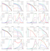 |
Fig. 2. Numerical results for four cases in the second group shown in Table 1. |
| In the text | |
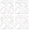 |
Fig. 3. Numerical results for four cases in the third group shown in Table 1. |
| In the text | |
|
Fig. 4. Theoretical modeling of light curves and Ep evolutions for GRB 110529A and GRB 090227B. In each diagram, numerical results are shown with blue (for flux) and red (for Ep) lines, while the observational data are presented by blue (for flux) and red (for Ep) dots. The gray histogram shows the photon-count light curve in a scaled way. |
| In the text | |
|
Fig. 5. Representative results of the prompt optical emission from three cases in Table 1. There are three light curves in different energy bands in the diagram of each case, including 2 eV, 1 keV, and 10 keV. |
| In the text | |
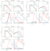 |
Fig. 6. Numerical results for three cases shown in Table C.1. |
| In the text | |
Current usage metrics show cumulative count of Article Views (full-text article views including HTML views, PDF and ePub downloads, according to the available data) and Abstracts Views on Vision4Press platform.
Data correspond to usage on the plateform after 2015. The current usage metrics is available 48-96 hours after online publication and is updated daily on week days.
Initial download of the metrics may take a while.