© The Authors 2025

1. Introduction

Gamma-ray burst (GRB) prompt emission is produced by internal dissipation in a relativistic ejecta (Sari & Piran 1997). However, the complete picture that accommodates the observed properties remains elusive, largely due to unknowns in the jet composition and the dissipation mechanism. Dissipation can start below the photosphere, leading to a non-thermal photospheric component (see e.g. Rees & Mészáros 2005; Giannios & Spruit 2007; Giannios 2008; Beloborodov 2010; Ryde et al. 2011; Vurm & Beloborodov 2016; Samuelsson et al. 2022). Otherwise, the photospheric emission is quasi-thermal (see e.g. Pe’er & Zhang 2006; Pe’er 2008; Beloborodov 2010; Acuner et al. 2020) and remains weak if the initial magnetisation is large (Daigne & Mochkovitch 2002; Hascoët et al. 2013). In this case, the dominant non-thermal component of the prompt GRB spectrum is emitted above the photosphere in internal shocks (Rees & Meszaros 1994; Kobayashi et al. 1997; Daigne & Mochkovitch 1998) or magnetic reconnection (see e.g. Thompson 1994; Spruit et al. 2001; Drenkhahn & Spruit 2002; Zhang & Yan 2011; McKinney & Uzdensky 2012), depending on the magnetisation of the ejecta at large distance. Synchrotron radiation from accelerated electrons is then a natural expectation, but it seems to be in tension with the observed low-energy photon index in prompt GRB spectra α (Band et al. 1993), which is usually well above the expected value of −3/2 in the radiatively efficient regime (Sari et al. 1998). This problem was identified in the GRB spectra measured by the Burst and Transient Source Experiment (BATSE) on board the Compton Gamma Ray Observatory (CGRO) (Cohen et al. 1997; Preece et al. 1998; Ghisellini et al. 2000) and has been confirmed by the Fermi Gamma-Ray Burst Monitor (GBM), which currently provides broad spectral information from the hard X-ray to the soft gamma-ray energy range (8 keV–40 MeV). In the latest GBM spectral catalogue, Poolakkil et al. (2021) reports a mean value of α ∼ −1.1 for the low-energy photon index resulting from the time-integrated spectral fits, and Yu et al. (2016) obtains a harder mean value, α ∼ −0.8, for the time-resolved spectral fits of the brightest bursts observed by the Fermi GBM.

Several processes have been proposed to explain the high values of the observed low-energy photon indices in the context of synchrotron models. In the fast cooling regime, inverse Compton scatterings in the Klein-Nishina regime affect the electron cooling, leading to steeper slopes (in νF_ν) of the synchrotron spectrum and reaching a low-energy photon index of α ∼ −1 (Derishev et al. 2001; Nakar et al. 2009; Bošnjak et al. 2009; Wang et al. 2009; Daigne et al. 2011; Barniol Duran et al. 2012). This also leads to a new high-energy spectral component that may explain the additional component detected by the Fermi Large Area Telescope (LAT; ∼20 MeV to more than 300 GeV) in the prompt emission of some bright GRBs (Ackermann et al. 2013; Ajello et al. 2019). Except in rare cases such as GRB 090926A (Ackermann et al. 2011; Yassine et al. 2017), this additional prompt high-energy component can usually only be fitted by a power law, which prevents a detailed comparison to radiative models.

Even higher values of the low-energy photon index in soft gamma rays (as high as α = −2/3) can be measured while maintaining a high radiative efficiency in the regime of marginally fast cooling synchrotron radiation suggested by Daigne et al. (2011), Beniamini & Piran (2013). Why this radiative regime would be common in GRBs, however, remains to be understood. In this paper, we investigate if this regime could naturally result from the magnetic field evolution from the electron acceleration site to larger scales.

The question of the intensity and structure of the magnetic field in the emission region is complex and can have a major influence on the synchrotron radiation from accelerated electrons. Most models for the relativistic ejection by the central engine imply a large-scale magnetic field anchored in the source with a high initial magnetisation (see e.g. Spruit et al. 2001; Tchekhovskoy et al. 2008, 2010; Granot et al. 2011; Gottlieb et al. 2022). On the other hand, the remaining magnetisation at large distance, where the dissipation responsible for the prompt emission occurs, is debated. In addition, the dissipation process itself strongly affects the magnetic field at much smaller scales. Shocks, expected if the large-scale magnetisation at large distance is low, generate a turbulent magnetic field in the shocked region by various plasma instabilities (see e.g. Sironi et al. 2013; Crumley et al. 2019; Bykov et al. 2022 in the mildly relativistic regime relevant for internal shocks). Reconnection, expected when the large-scale magnetisation at large distance is high, dissipates the magnetic field and produces a new complex structure in the current sheets, including the formation of magnetic islands (see e.g. Drake et al. 2006; Sironi & Spitkovsky 2014). Particle-in-cell (PIC) simulations provide a self-consistent description of such processes in shocks and reconnection layers that are coupled to the particle acceleration (for recent reviews, see e.g. Marcowith et al. 2020; Vanthieghem et al. 2020) and magnetic field amplification (see e.g. Silva et al. 2003; Medvedev et al. 2005). Moreover, PIC simulations of relativistic shocks show a very fast decay of the generated magnetic field on a scale comparable with the simulation box size, (Chang et al. 2008; Keshet et al. 2009; Lemoine et al. 2019; Vanthieghem et al. 2020), which nevertheless remains limited to at most several thousand times the plasma skin depth (see e.g. Keshet et al. 2009; Sironi & Spitkovsky 2014; Crumley et al. 2019), (i.e. a size many orders of magnitude smaller than the geometrical size of the ejecta). The length travelled by radiating electrons responsible for the soft gamma-ray synchrotron component is much longer than this plasma scale, but it is also much smaller than the geometrical size of the ejecta when these electrons are fast cooling. This means that the magnetic field in which these electrons radiate is not described by current simulations, neither relativistic magnetohydrodynamic (MHD) simulations of the whole ejecta nor PIC simulations of the dissipative region. The intensity and structure of the magnetic field on this intermediate scale, relevant for the radiation, is a matter of debate. It can be affected by several additional physical processes and may therefore differ strongly from the extrapolation of the structure observed in current PIC simulations, with a decay scale much larger than the plasma scale (see e.g. Derishev & Piran 2016, and references therein). This paper explores the impact of a possible evolution of the magnetic field intensity on the observed synchrotron spectrum at these intermediate scales and precisely studies if a magnetic field decay can naturally lead to the marginally fast cooling regime.

Several authors have already suggested models for the prompt and afterglow GRB emission where the magnetic field decays on a length scale significantly smaller than the geometrical width of the ejecta: Rossi & Rees (2003), Lemoine (2013) for the afterglow spectrum and Pe’er & Zhang (2006), Derishev (2007), Zhao et al. (2014), Zhou et al. (2023) for the prompt spectrum. Following these early studies, we investigate the effect of such a magnetic field evolution on GRB prompt spectra, taking into account in a numerical approach both the synchrotron radiation and the synchrotron self-Compton (SSC) scatterings and exploring a large parameter space.

In Sect. 2, we discuss the cooling of electrons in a decaying magnetic field. Using a numerical radiative code, we study in Sect. 3 the additional impact of inverse Compton scatterings, and in Sect. 4, we explore the parameter space describing the physical conditions in the co-moving frame of the emission region. We also discuss the consequences of the magnetic field decay on the light curves and spectra as well as on the spectral evolution in the specific case of internal shocks. Finally, we discuss in Sect. 5 our results and compare them to observations, and we summarise our conclusions.

2. Synchrotron radiation in a decaying magnetic field

2.1. Expected effect of a decaying magnetic field

We assumed that electrons are accelerated in a region where the magnetic field is B′₀, corresponding to a magnetic energy density u_B, 0 = B′₀²/8π, and reach a power-law distribution with a minimum Lorentz factor Γ_m and a slope −p. The discussion in this section is entirely done in the co-moving frame of the emitting region. Electrons with a Lorentz factor γ will radiate their energy on the synchrotron timescale

$$\begin{array}{c}\hfill t_{\mathrm{syn}}^{\prime }(\gamma )=t_{\mathrm{dyn}}^{\prime }\frac{{\mathrm{\Gamma }}_{\mathrm{c},0}}{\gamma },\end{array}$$(1)

where Γ_c, 0 is defined as the Lorentz factors of electrons in the magnetic field B′₀ that have a synchrotron timescale equal to the timescale of the adiabatic cooling (dynamical timescale):

$$\begin{array}{c}\hfill {\mathrm{\Gamma }}_{\mathrm{c},0}=\frac{6\pi m_{\mathrm{e}}c}{{\sigma }_{\mathrm{T}}{B^{\prime }}_0^2{t}_{\mathrm{dyn}}^{\prime }}·\end{array}$$(2)

In the fast cooling regime (Γ_m ≫ Γ_c, 0), all electrons radiate efficiently by the synchrotron process. In this case, if the magnetic field is constant (B′=B′₀), the peak of the synchrotron spectrum occurs at the synchrotron frequency of electrons at Γ_m, namely, 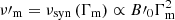$\nu {\prime }_{\mathrm{m}}={\nu }_{\mathrm{syn}}\left({\mathrm{\Gamma }}_{\mathrm{m}}\right)\propto B{\prime }_0{\mathrm{\Gamma }}_{\mathrm{m}}^2$, and the photon index below the peak is α = −3/2 (Sari et al. 1998). A photon index −2/3 (corresponding to a steeper slope 4/3 in νF_ν) is recovered at a very low frequency below $\nu {\prime }_{\mathrm{c},0}={\nu }_{\mathrm{syn}}\left({\mathrm{\Gamma }}_{\mathrm{c},0}\right)=\nu {\prime }_{\mathrm{m}}{({\mathrm{\Gamma }}_{\mathrm{c},0}/{\mathrm{\Gamma }}_{\mathrm{m}})}^2\ll \nu {\prime }_{\mathrm{m}}$. Therefore, the standard fast cooling synchrotron spectrum predicts a low-energy photon index of α = −3/2, which is lower than what is usually observed (Poolakkil et al. 2021).

A possibility to solve this problem without decreasing the radiative efficiency, which should remain high in gamma-ray bursts to explain the observed luminosities, has been proposed by Daigne et al. (2011) and Beniamini & Piran (2013): In the marginally fast cooling regime, where the cooling break $\nu {\prime }_{\mathrm{c},0}$ is very close to the peak $\nu {\prime }_{\mathrm{m}}$, the intermediate branch of the spectrum with slope −3/2 disappears, and the large value α = −2/3 is recovered. However, maintaining the condition Γ_c, 0 ≃ (0.1 − 1)Γ_m during most of the prompt GRB emission may require some kind of fine-tuning of the microphysics parameters.

In this paper, we describe how this marginally fast cooling regime can naturally emerge if electrons radiate in a decaying magnetic field. More precisely, we consider the case where the magnetic field is not constant but rather decays outside the acceleration site over a timescale $t{\prime }_{\mathrm{B}}$. An electron escaping the acceleration site will radiate in this decaying magnetic field. If $t{\prime }_{\mathrm{B}}$ is large compared to 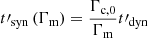$t{\prime }_{\mathrm{syn}}\left({\mathrm{\Gamma }}_{\mathrm{m}}\right)=\frac{{\mathrm{\Gamma }}_{\mathrm{c},0}}{{\mathrm{\Gamma }}_{\mathrm{m}}}t{\prime }_{\mathrm{dyn}}$, electrons with a Lorentz factor γ ≳ Γ_m will still experience a magnetic field of the order of B′₀, and the peak and the high-energy part of the synchrotron spectrum will not be affected. On the other hand, if $t{\prime }_{\mathrm{B}}<t{\prime }_{\mathrm{dyn}}$, electrons with Lorentz factors Γ_c, 0 < γ < Γ_m will lose their energy more slowly than expected because they will meet a lower magnetic field when they start to travel outside the initial acceleration site. This will affect the low-energy part of the synchrotron spectrum, as the cooling break will increase to ${\nu }_{\mathrm{c}}\simeq {\nu }_{\mathrm{c},0}{(t{\prime }_{\mathrm{dyn}}/t{\prime }_{\mathrm{B}})}^2$. It allows the synchrotron radiation to naturally tend towards the marginally fast cooling regime. Indeed, there are usually several orders of magnitude between the radiative timescale at Γ_m and the dynamical timescale so that the necessary condition for the proposed scenario to work, $t{\prime }_{\mathrm{syn}}({\mathrm{\Gamma }}_{\mathrm{m}})<t{\prime }_{\mathrm{B}}<t{\prime }_{\mathrm{dyn}}$, is not very constraining. Therefore, a rapidly decaying magnetic field is a promising possibility to recover a photon index of α ∼ −2/3 in the synchrotron fast cooling regime without reducing the radiative efficiency, as it will remain high as long as $t{\prime }_{\mathrm{B}}\gg t{\prime }_{\mathrm{syn}}({\mathrm{\Gamma }}_{\mathrm{m}})$ (i.e. $t{\prime }_{\mathrm{B}}/t{\prime }_{\mathrm{dyn}}\gg {\mathrm{\Gamma }}_{\mathrm{c},0}/{\mathrm{\Gamma }}_{\mathrm{m}}$). This leads to the final condition for the regime described in this paper:

$$\begin{array}{c}\hfill \frac{{\mathrm{\Gamma }}_{\mathrm{c},0}}{{\mathrm{\Gamma }}_{\mathrm{m}}}\lesssim \frac{t_{\mathrm{B}}^{\prime }}{t_{\mathrm{dyn}}^{\prime }}\lesssim 1.\end{array}$$(3)

We note that if the magnetic field decays extremely fast ($t{\prime }_{\mathrm{B}}/t{\prime }_{\mathrm{dyn}}<{\mathrm{\Gamma }}_{\mathrm{c},0}/{\mathrm{\Gamma }}_{\mathrm{m}}$), the low-energy photon index α = −2/3 is still recovered, but all electrons may be slow cooling, leading to a lower radiative efficiency. On the other hand, if $t{\prime }_{\mathrm{B}}/t{\prime }_{\mathrm{dyn}}>1$, the observed spectrum is mostly unaffected by the magnetic field decay.

2.2. Prescription for the magnetic field decay

In the following we explore the mechanism described above by assuming a simple prescription for the magnetic field decay:

$$\begin{array}{c}\hfill B^{\prime }(t^{\prime })=B_0^{\prime }{e}^{-t^{\prime }/t_{\mathrm{B}}^{\prime }}.\end{array}$$(4)

Derishev (2007), Lemoine (2013), Panaitescu (2019) instead considered a power-law decay of the magnetic field. Such a power-law decay is indeed seen in some PIC simulations (see e.g. Vanthieghem et al. 2020) but at a scale that is much lower than the one considered here. Derishev & Piran (2016) studied the effect of intrinsic pair loading in relativistic shocks, which can lead to a magnetic field decay on a much larger scale. They assumed either an exponential decay as in Eq. (4) or a power-law decay. We tested a power-law prescription, namely, B′=B′₀ for $t\prime \le t{\prime }_{\mathrm{B}}$ and $B\prime =B{\prime }_0{(t\prime /t{\prime }_{\mathrm{B}})}^{-x}$ for $t\prime >t{\prime }_{\mathrm{B}}$, with power-law indices x comparable to those used in Lemoine et al. (2013), and we found that this does not significantly change the conclusions obtained when adopting Eq. (4). Therefore, we only consider Eq. (4) in the following, as it introduces a single new parameter, the timescale $t{\prime }_{\mathrm{B}}$, rather than two parameters in the case of a power law.

The regime of synchrotron radiation in a rapidly decaying magnetic field discussed in the present paper is similar to the scenario proposed by Pe’er & Zhang (2006), Derishev (2007), Zhao et al. (2014) for the GRB prompt emission and Rossi & Rees (2003), Lemoine (2013) for the GRB afterglow. In the context of the GRB prompt emission, Pe’er & Zhang (2006) described the effect of a decaying magnetic field on the prompt synchrotron spectrum and gave some orders of magnitude for the expected timescales to show that $t{\prime }_{\mathrm{B}}<t{\prime }_{\mathrm{syn}}$ could indeed be expected in certain conditions in GRBs. Then Zhao et al. (2014) presented a first calculation of the radiated spectrum in this scenario in the context of the internal shock model. They used the prescription given by Eq. (4) and also considered a power-law decay, but they made some simplifications: adiabatic cooling is not included, which leads to an overestimate of the radiative efficiency, as it prevents the synchrotron radiation from entering too much into the slow cooling regime, and the Klein-Nishina corrections are not included for the inverse Compton scatterings, whereas they are usually important in the GRB prompt emission phase (Bošnjak et al. 2009; Zou et al. 2009; Piran et al. 2009). The present paper aims at exploring the same scenario without these simplified assumptions. Using the same assumptions as Zhao et al. (2014), Zhou et al. (2023) studied the additional effect of a background magnetic field. However, they focused on a very fast decay, $t{\prime }_{\mathrm{B}}/t{\prime }_{\mathrm{dyn}}\ll {\mathrm{\Gamma }}_{\mathrm{c},0}/{\mathrm{\Gamma }}_{\mathrm{m}}$. As we focus here on less rapid decays (see condition given by Eq. 3), the effect of such a background field $B{\prime }_{\mathrm{bkg}}$ should be weak as long as the ratio $f_{\mathrm{B}}={(B{\prime }_{\mathrm{bkg}}/B{\prime }_0)}^2$ is not too large. For this reason, we do not include a background magnetic field in the present study, which avoids having to introduce an additional free parameter in the model.

We note that Uhm & Zhang (2014), Geng et al. (2018), Wang & Dai (2021) also discussed the synchrotron radiation of electrons in a decaying magnetic field in the context of the prompt GRB emission. However, their scenario is very different from the situation with a rapid decay studied here. It corresponds to a slow decay of the magnetic field governed by the large-scale dynamics of the emission zone. Indeed their prescription is B′=B′₀(r/r₀)^−b, with b = 1.0 − 1.5 and where r₀ is the radius where electrons were accelerated (a passive field in a conical jet corresponds to b = 1; see e.g. Spruit et al. 2001). This corresponds to a characteristic timescale of $t{\prime }_{\mathrm{B}}=t{\prime }_{\mathrm{dyn}}/b$ (with $t{\prime }_{\mathrm{dyn}}=\frac{r_0}{{\mathrm{\Gamma }}_{0}c}$) that is much larger than what is considered in the present study. In this scenario, the ratio $t{\prime }_{\mathrm{B}}/t{\prime }_{\mathrm{dyn}}\simeq 0.7-1$ is very close to the upper limit of the condition given by Eq. (3). Therefore, the steepest spectra with a photon index of α → −2/3 are obtained by Uhm & Zhang (2014) by reaching the marginally fast cooling regime with some fine-tuning of the initial value B′₀ of the magnetic field to get Γ_c/Γ_m ∼ 0.1 − 1. For instance, the choice of values considered in the reference case in Uhm & Zhang (2014) (see their Figs. 1 and 2) corresponds to Γ_c/Γ_m ≃ 0.08. Yan et al. (2024) have recently developed a model of a single pulse in a GRB light curve based on the synchrotron radiation of accelerated electrons in a relativistic shell with a decaying magnetic field using the prescription from Uhm & Zhang (2014). They successfully fit the time-resolved gamma-ray spectra of observed pulses with this model (see also Zhang et al. 2016; Yang et al. 2023). However, their best-fit parameters correspond in many cases to a ratio Γ_c, 0/Γ_m ∼ 0.1 − 1. This confirms that the marginally fast cooling regime is required to reproduce the data in a significant fraction of GRB pulses, but the values of the parameters confirm that some fine-tuning is required to reach this radiative regime, due to the slow decay of the magnetic field. Finally Geng et al. (2018) obtained results similar to those of Uhm & Zhang (2014) with a calculation extended to include inverse Compton scatterings. In most of their examples, the scatterings in the Klein-Nishina regime have a stronger impact on the spectrum than the slow decay of the magnetic field, leading to a low-energy photon index of α → 1, which is in agreement with Derishev et al. (2001), Nakar et al. (2009), Bošnjak et al. (2009), Daigne et al. (2011) (see also Sect. 2.4).

2.3. Calculation of the synchrotron radiation

We assumed that the acceleration mechanism proceeds on a timescale much shorter than all other timescales considered here¹. Therefore, we adopted a power law for the initial distribution of electrons at t′ = 0:

$$\begin{array}{c}\hfill n(\gamma ,0)=(p-1)\frac{n_{\mathrm{e}}^{\mathrm{acc}}}{{\mathrm{\Gamma }}_{\mathrm{m}}}{\left(\frac{\gamma }{{\mathrm{\Gamma }}_{\mathrm{m}}}\right)}^{-p},\end{array}$$(5)

where $n_{\mathrm{e}}^{\mathrm{acc}}$ is the density of accelerated electrons in the co-moving frame. This corresponds to an initial energy of

$$\begin{array}{c}\hfill u_{\mathrm{e}}=\frac{p-1}{p-2}{n}_{\mathrm{e}}^{\mathrm{acc}}{\mathrm{\Gamma }}_{\mathrm{m}}{m}_{\mathrm{e}}{c}^2\end{array}$$(6)

injected into non-thermal electrons. If we neglect all radiative processes except for synchrotron emission, each electron evolves according to

$$\begin{array}{c}\hfill \frac{\mathrm{d}\gamma }{\mathrm{d}{t}^{\prime }}=-\frac{\gamma }{t_{\mathrm{dyn}}^{\prime }}-\frac{1}{{\mathrm{\Gamma }}_{\mathrm{c},0}}\frac{{\gamma }^2}{t_{\mathrm{dyn}}^{\prime }}{e}^{-2\frac{t^{\prime }}{t_{\mathrm{B}}^{\prime }}},\end{array}$$(7)

where the first term stands for adiabatic cooling over the timescale $t{\prime }_{\mathrm{dyn}}$ and the second term stands for the synchrotron radiation in a decaying magnetic field, using the prescription given by Eq. (4) and the definition of Γ_c, 0 given by Eq. (2). The solution for an electron with Lorentz factor γ₀ is

$$\begin{array}{c}\hfill \gamma (t^{\prime })={\gamma }_0\frac{e^{-t^{\prime }/t_{\mathrm{dyn}}^{\prime }}}{1+\frac{{\gamma }_0}{{\mathrm{\Gamma }}_{\mathrm{c},0}}\frac{1}{1+2\frac{t_{\mathrm{dyn}}^{\prime }}{t_{\mathrm{B}}^{\prime }}}(1-e^{-(\frac{1}{t_{\mathrm{dyn}}^{\prime }}+\frac{2}{t_{\mathrm{B}}^{\prime }})t^{\prime }})}·\end{array}$$(8)

In the standard case (constant magnetic field, $t{\prime }_{\mathrm{B}}\gg t{\prime }_{\mathrm{dyn}}$), the Lorentz factor of a given electron for $t\prime =t{\prime }_{\mathrm{dyn}}$ equals ∼Γ_c, 0 for γ₀ ≫ Γ_c, 0 (fast cooling electron) and ∼γ₀ otherwise (slow cooling electron). In presence of a decaying magnetic field with $t{\prime }_{\mathrm{B}}\ll t{\prime }_{\mathrm{dyn}}$, it appears clearly from Eq. (8) that $\gamma (t{\prime }_{\mathrm{dyn}})\sim {\mathrm{\Gamma }}_{\mathrm{c},0}$ for ${\gamma }_0\gg {\mathrm{\Gamma }}_{\mathrm{c},0}\frac{t{\prime }_{\mathrm{dyn}}}{t{\prime }_{\mathrm{B}}}$. Therefore, electrons radiate efficiently only above an effective critical Lorentz factor

$$\begin{array}{c}\hfill {\mathrm{\Gamma }}_{\mathrm{c},\mathrm{eff}}\simeq \frac{t_{\mathrm{dyn}}^{\prime }}{t_{\mathrm{B}}^{\prime }}{\mathrm{\Gamma }}_{\mathrm{c},0},\end{array}$$(9)

which leads to an increase of the cooling break frequency by a factor of ${(t{\prime }_{\mathrm{dyn}}/t{\prime }_{\mathrm{B}})}^2$, as described above. We note that for an extreme decay, namely, $t{\prime }_{\mathrm{B}}/t{\prime }_{\mathrm{dyn}}\ll \frac{{\mathrm{\Gamma }}_{\mathrm{c},0}}{{\mathrm{\Gamma }}_{\mathrm{m}}}$, we expect a slow cooling spectrum even for Γ_m > Γ_c, 0, in agreement with Eq. (3).

From the solution given by Eq. (8), the electron distribution $n(\gamma ,t\prime )=n({\gamma }_0,0)\frac{\mathrm{d}{\gamma }_0}{\mathrm{d}\gamma }$ can be computed at any time t′, and the final radiated energy by the synchrotron process can be deduced by integrating the synchrotron power over $t{\prime }_{\mathrm{dyn}}$:

$$\begin{array}{c}\hfill u_{\mathrm{syn}}={\displaystyle {\int }_0^{t_{\mathrm{dyn}}^{\prime }}}\mathrm{d}{t}^{\prime }{\displaystyle \int \mathrm{d}}\gamma n(\gamma ,t^{\prime })\frac{m_{\mathrm{e}}{c}^2}{{\mathrm{\Gamma }}_{\mathrm{c},0}}\frac{{\gamma }^2}{t_{\mathrm{dyn}}^{\prime }}{e}^{-2\frac{t^{\prime }}{t_{\mathrm{B}}^{\prime }}}.\end{array}$$(10)

The corresponding spectrum u_ν′ can also be computed by integrating the synchrotron power at frequency ν′:

$$\begin{array}{c}\hfill u_{{\nu }^{\prime }}={\displaystyle {\int }_0^{t_{\mathrm{dyn}}^{\prime }}}\mathrm{d}{t}^{\prime }{\displaystyle \int \mathrm{d}\gamma }n(\gamma ,t^{\prime })P_{\mathrm{syn},{\nu }^{\prime }}(\gamma ;B^{\prime }(t^{\prime })).\end{array}$$(11)

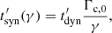
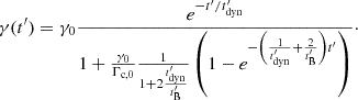
This is done in a first step using a simplified shape for the synchrotron spectrum of a single electron with Lorentz factor γ: a power law with a slope of 1/3 up to ν_syn(γ) and zero above. The result is plotted in blue in Fig. 1 for Γ_m/Γ_c, 0 = 300 with a constant magnetic field (dotted line) and with a decaying magnetic field with $t{\prime }_{\mathrm{B}}/t{\prime }_{\mathrm{syn}}={10}^{-2}$ (solid line), which fulfils the condition given by Eq. (3). For the constant magnetic field, we obtained the standard fast cooling synchrotron spectrum described by Sari et al. (1998), with a photon index of α = −3/2 below the peak at $\nu {\prime }_{\mathrm{m}}$ and a photon index of −2/3 below the cooling break $\nu {\prime }_{\mathrm{c}}\simeq {10}^{-5}\nu {\prime }_{\mathrm{m}}$. For the decaying magnetic field, the effective cooling break is at $\nu {\prime }_{\mathrm{c}}=\nu {\prime }_{\mathrm{c},0}{(t{\prime }_{\mathrm{dyn}}/t{\prime }_{\mathrm{B}})}^2\sim {10}^4\nu {\prime }_{\mathrm{c},0}$ so that the intermediate spectral branch with index −3/2 disappears and the photon index α = −2/3 is measured immediately below the peak, which is still at $\nu {\prime }_{\mathrm{m}}$.

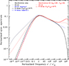Fig. 1. Effect of a decaying magnetic field on the synchrotron spectrum. The normalised spectrum ν′uν′/ue is plotted as a function of the normalised frequency $\nu \prime /\nu {\prime }_{\mathrm{m}}$ for a constant magnetic field (dotted line) or a decaying magnetic field on a timescale $t{\prime }_{\mathrm{B}}={10}^{-2}t{\prime }_{\mathrm{dyn}}$ (solid line). The calculation has been done with the numerical radiative code described in Sect. 2.4 either including only the synchrotron process (black) or both the synchrotron radiation and the inverse Compton scatterings (red). The following parameters were adopted: Γc, 0 = Γm/300, YTh = 10, wm = 102, and p = 2.5. In the synchrotron-only case, the result of the approximate calculation discussed in Sect. 2.3 is plotted in blue for comparison.

2.4. Additional effects: The role of inverse Compton scatterings

In a more realistic approach, other radiative processes cannot be neglected. This is especially true for inverse Compton scatterings, which can strongly affect the cooling of electrons. In the fast cooling regime, Bošnjak et al. (2009), Daigne et al. (2011) have shown that the effect on the synchrotron spectral component is governed by two parameters (see also Nakar et al. 2009):

$$\begin{array}{c}\hfill Y_{\mathrm{Th}}=\frac{4}{3}{\mathrm{\Gamma }}_{\mathrm{m}}^2\left({\sigma }_{\mathrm{T}}{n}_{\mathrm{e}}^{\mathrm{acc}}c{t}_{\mathrm{syn}}^{\prime }\left({\mathrm{\Gamma }}_{\mathrm{m}}\right)\right)=\frac{p-2}{p-1}\frac{u_{\mathrm{e}}}{u_{\mathrm{B},0}},\end{array}$$(12)

which governs the efficiency of scatterings, and

$$\begin{array}{c}\hfill w_{\mathrm{m}}={\mathrm{\Gamma }}_{\mathrm{m}}\frac{h{\nu }_{\mathrm{m}}^{\prime }}{m_{\mathrm{e}}{c}^2},\end{array}$$(13)

which measures how important Klein-Nishina corrections are (Thomson regime corresponds to w_m ≪ 1). In particular, Derishev et al. (2001), Nakar et al. (2009), Daigne et al. (2011) identified that for Y_Th ≫ 1 and w_m ≫ 1, a photon index of α ≲ −1 is obtained below $\nu {\prime }_{\mathrm{m}}$ in the synchrotron component.

Using the radiative code described in Bošnjak et al. (2009), where a decaying magnetic field following Eq. (4) has been implemented, we can solve the evolution of the distribution of electrons and the corresponding emitted spectrum in the more realistic case where inverse Compton scatterings are taken into account. This code computes simultaneously the evolution of the electron and photon distribution, taking into account all relevant processes: adiabatic cooling, synchrotron radiation, synchrotron self-absorption, inverse Compton scatterings (full treatment including the Klein-Nishina regime), and photon-photon annihilation at high energy (see Bošnjak et al. 2009 for a complete description). The secondary pairs produced by the latter process are not included. We therefore limited our study to cases where the absorption of gamma-ray photons remains weak.

This more realistic calculation is shown in Fig. 1 for the same example as before, using Y_Th = 10 and w_m = 100 and including adiabatic cooling, synchrotron radiation, and inverse Compton scatterings (red curves). For comparison, the synchrotron-only case is also plotted with the same radiative code (black line), and it agrees well with the simple calculation presented in Sect. 2.3. When inverse Compton scatterings are included, a larger photon index of α ∼ −1.2 is found in the case of a constant magnetic field due to the effect of scatterings in the Klein-Nishina regime, which is in agreement with Daigne et al. (2011). However, an even larger index of α = −2/3 is obtained when the decay of the magnetic field is included. We note that the inverse Compton scatterings are also modified, and we discuss the implications for the high-energy prompt emission from gamma-ray bursts at a later point. In the following, all results are produced with this same numerical radiative code.

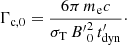
3. Exploring the effect of the magnetic field decay in different inverse Compton regimes

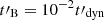
Next, we explore the parameter space of the synchrotron radiation with a decaying magnetic field. This is done with the same radiative code as in Sect. 2.4, which includes adiabatic cooling, synchrotron radiation, and inverse Compton scattering. Figure 2 shows the evolution of the synchrotron spectrum as a function of Y_Th for four different values of w_m, corresponding to different regimes for inverse Compton scatterings, from the full Thomson regime to the strong Klein-Nishina regime, and using either a constant magnetic field (this case is similar to Fig. 2 in Daigne et al. 2011) or a decaying magnetic field with $t{\prime }_{\mathrm{B}}/t{\prime }_{\mathrm{dyn}}={10}^{-1}$ or $t{\prime }_{\mathrm{B}}/t{\prime }_{\mathrm{dyn}}={10}^{-2}$. The initial ratio Γ_c, 0/Γ_m is fixed to 1/300. In the case of a constant magnetic field (black lines), we recovered the results from Daigne et al. (2011). In particular, a photon index of α > −1.5 was found for w_m > 1 and Y_Th > 1. The limit α → −1 was reached for w_m = 10² − 10⁴ and Y_Th ≳ w_m. However, as expected from the discussion in Sect. 2, even larger photon indices are found if the magnetic field is decaying, regardless of the values of w_m and Y_Th. Therefore, the effect of a magnetic field decay appears as a robust mechanism to produce a large photon index (i.e. a steep slope in νF_ν) in the synchrotron component of the spectrum.

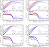Fig. 2. Effect of a decaying magnetic field on the synchrotron spectrum: Realistic case including inverse Compton scatterings. The normalised synchrotron spectrum νuν/ue as well as the photon index are plotted as a function of the normalised frequency $\nu \prime /\nu {\prime }_{\mathrm{m}}$ for a constant magnetic field (black) or a decaying magnetic field on a timescale of $t{\prime }_{\mathrm{B}}/t{\prime }_{\mathrm{dyn}}={10}^{-1}$ (red) and 10−2 (blue). The calculation includes adiabatic cooling, synchrotron radiation, and inverse Compton scatterings but does not take into account synchrotron self-absorption and pair production. Each panel corresponds to a different value of the parameter wm, which measures the importance of Klein-Nishina effects, from 10−2 (Thomson regime) to 104 (strong Klein-Nishina regime). The spectra are plotted for YTh = 10−1, 1, 10, 102, 103, and 104, which corresponds to an increasing efficiency of scatterings (see text). We assumed everywhere an electron slope p = 2.5 and a magnetic field B′0 in the acceleration site corresponding to Γc/Γm = 1/300.

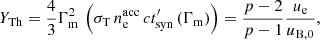
3.1. Photon index and radiative efficiency

Figure 3 shows the value of the photon index below the peak of the synchrotron spectrum in a plane $t{\prime }_{\mathrm{B}}/t{\prime }_{\mathrm{dyn}}$ versus Γ_c, 0/Γ_m for five different sets of the two parameters (Y_Th, w_m) governing the inverse Compton scatterings². In this diagram, the standard assumption of a constant magnetic field is recovered at the top, when $t{\prime }_{\mathrm{B}}\gg t{\prime }_{\mathrm{dyn}}$. Lines of constant radiative efficiency,

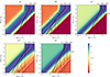Fig. 3. Synchrotron emission within a decaying magnetic field: Parameter space. In the $t{\prime }_{\mathrm{B}}/t{\prime }_{\mathrm{dyn}}$ vs Γc, 0/Γm plane, the value of the low-energy photon index α of the synchrotron spectrum is colour-coded. In this plane, the standard synchrotron spectrum with a constant magnetic field is at the top ($t{\prime }_{\mathrm{B}}\to \infty$). In this case the fast cooling regime is on the left (Γc, 0 ≪ Γm), while the marginally fast cooling regime is on the right (Γc, 0 ≃ Γm). Black solid lines indicate the limits of the high radiative efficiency region (thick: frad = 0.9; thin: frad = 0.5; very thin: fdad = 0.1). Contours of the inverse Compton/synchrotron ratio Lic/Lsyn are plotted with black dashed lines. Each panel corresponds to a set of values for the parameters YTh, 0 and wm that govern the importance of inverse Compton scatterings and Klein-Nishina corrections. (a) YTh, 0 = 0.1; wm = 10−2. (b) YTh, 0 = 0.1; wm = 102. (c) YTh, 0 = 102; wm = 102. (d) YTh, 0 = 102; wm = 104. (e) YTh, 0 = 104; wm = 104.

$$\begin{array}{c}\hfill f_{\mathrm{rad}}=\frac{1}{u_{\mathrm{e}}}{\displaystyle {\int }_0^{\infty }}{u}_{{\nu }^{\prime }}\mathrm{d}{\nu }^{\prime },\end{array}$$(14)

are also plotted. The gamma-ray burst prompt emission must correspond most of the time to a high radiative efficiency to be able to reproduce the observed huge gamma-ray energies and the short timescale variability (Rees & Meszaros 1994; Sari et al. 1996; Kobayashi et al. 1997). Figure 3 shows clearly that in the efficient region (f_rad ≳ 0.5) the photon index spans a broad range of values, from the standard fast cooling value −3/2 to a maximum value of −2/3. Interestingly, the marginally fast cooling regime α ≃ −2/3 is found in a large region of the parameter space. It can be compared to Fig. 5 in Daigne et al. (2011), where this regime was explored for a constant magnetic field and then required some fine-tuning of the parameters to maintain a high radiative efficiency (Γ_c, 0/Γ_m ≃ 0.1 − 1).

Our numerical calculation shows that the effect of a decaying magnetic field is robust: steep slopes in νF_ν are found for low ratios Γ_c, 0/Γ_m and for all values of Y_Th. More precisely:

• The largest value of the photon index, α ∼ −2/3 (marginally fast cooling), is obtained for a rapid decay with

  $$\begin{array}{c}\hfill 0.1\frac{{\mathrm{\Gamma }}_{\mathrm{c},0}}{{\mathrm{\Gamma }}_{\mathrm{m}}}\lesssim \frac{t_{\mathrm{B}}^{\prime }}{t_{\mathrm{dyn}}^{\prime }}\lesssim 10\frac{{\mathrm{\Gamma }}_{\mathrm{c},0}}{{\mathrm{\Gamma }}_{\mathrm{m}}},\end{array}$$(15)

  in agreement with Sect. 2 (see Eq. (3)).

• Inverse Compton scatterings govern the value of α in the fast cooling regime for a slower decay with $\frac{t{\prime }_{\mathrm{B}}}{t{\prime }_{\mathrm{dyn}}}\gtrsim 10\frac{{\mathrm{\Gamma }}_{\mathrm{c},0}}{{\mathrm{\Gamma }}_{\mathrm{m}}}$ when they are negligible, panels a and b, the standard photon index α = −3/2 is recovered; the same value is also obtained when inverse Compton scatterings become important but occur in the Thomson regime (large Y_Th, low w_m, not shown in Fig. 3). Finally, when scatterings enter the Klein-Nishina regime, α increases towards −1, as already discussed in Daigne et al. (2011). These results are in agreement with the study by Geng et al. (2018), where $t{\prime }_{\mathrm{B}}/t{\prime }_{\mathrm{dyn}}\sim 1$.

• Much flatter νF_ν spectra (photon index −3/2 < α < −2) are obtained in the bottom-right region of the diagram for a very rapid decay ($\frac{t{\prime }_{\mathrm{B}}}{t{\prime }_{\mathrm{dyn}}}\lesssim 0.1\frac{{\mathrm{\Gamma }}_{\mathrm{c}}}{{\mathrm{\Gamma }}_{\mathrm{m}}}$). This is due to the fact that the magnetic field decays so fast that even electrons at Γ_m are affected (see corresponding spectra in Fig. 2). This means that the whole electron population enters the slow cooling regime, and the measured low-energy photon index is close to the expected value $-\frac{p+1}{2}$ (−1.75 for p = 2.5) of the intermediate branch between $\nu {\prime }_{\mathrm{m}}$ and $\nu {\prime }_{\mathrm{c}}$ in this case (Sari et al. 1998). As expected, the radiative efficiency falls in this region, which cannot correspond to the usual conditions during the GRB prompt emission. We note that a non-negligible background magnetic field can rapidly become dominant in this regime, which would affect the final spectral shape (see Zhou et al. 2023).

3.2. The high-energy component

In this section, we explore the effect of the magnetic field decay on the high-energy component due to inverse Compton scatterings. When the magnetic field decays, the Compton parameter Y_Th increases, which enhances the efficiency of the scatterings. However, two other effects must be taken into account: (i) Inverse Compton scatterings are expected to occur in the Klein-Nishina regime during the GRB prompt emission (Bošnjak et al. 2009; Piran et al. 2009). As the value of w_m depends only on the electron Lorentz factor Γ_m, it is not affected by the magnetic field decay. Therefore, the Klein-Nishina corrections remain strong for a large w_m even with a magnetic field decay. (ii) In the regime of interest discussed in this paper, the magnetic field decay is fast (i.e. $t{\prime }_{\mathrm{B}}<t{\prime }_{\mathrm{dyn}}$), but it still decays on a timescale that is too large to affect electrons at Γ_m ($t{\prime }_{\mathrm{B}}>t{\prime }_{\mathrm{syn}}({\mathrm{\Gamma }}_{\mathrm{m}})=({\mathrm{\Gamma }}_{\mathrm{c},0}/{\mathrm{\Gamma }}_{\mathrm{m}})t{\prime }_{\mathrm{dyn}}$) – we refer to condition given by Eq. (3). Thus, the magnetic field decay only affects the synchrotron spectrum below the peak (low-energy photon index α) and can only moderately affect the efficiency of the SSC component. On the other hand, the regime of very fast decay, that is, $t{\prime }_{\mathrm{B}}<t{\prime }_{\mathrm{syn}}({\mathrm{\Gamma }}_{\mathrm{m}})$, can lead to more efficient inverse Compton scatterings. However, this regime is not favoured by observations. Indeed we have shown above that the spectral shape of the synchrotron component is now also affected at the peak (flattening) and that the radiative efficiency is reduced (electrons can even enter the slow cooling regime).

To check this interpretation and quantitatively investigate the effect of the magnetic field decay on the high-energy component of the spectrum, lines of constant ratio of the inverse Compton luminosity over the synchrotron luminosity L_ic/L_syn are also plotted in Fig. 3. Interestingly, the region of steepest synchrotron spectra shows a large diversity of L_ic/L_syn ratios, depending on the regime of inverse Compton scatterings. The largest ratios, L_ic/L_syn ≃ 0.1 − 1, are obtained for large Y_Th and w_m ≲ Y_Th (Fig. 3, panels a, c, e). Much smaller values are obtained if Y_Th is small (L_ic/L_syn ≃ 10⁻² − 10⁻¹ in panel b) or if the Klein-Nishina reduction becomes strong (L_ic/L_syn ≃ 10⁻³ − 10⁻² in panel d). This may explain the observed diversity revealed by the Fermi satellite, as during the prompt phase, the ratio of the fluence at high energy (0.1−100 GeV) measured by the LAT instrument over the fluence at low energy (10 keV−1 MeV) measured by the GBM instrument is typically in the range 10⁻² − 1 in GRBs detected by the LAT (see Fig. 15 in the second Fermi-LAT GRB catalogue, Ajello et al. 2019), with probably even lower ratios for GBM bursts that are not detected by the LAT. Therefore, the scenario discussed in this paper to explain the shape of the soft gamma-ray spectrum in the GRB prompt emission is also compatible with the constraints on the L_IC/L_syn ratio provided by Fermi/LAT.

We note in Fig. 3 that there is a small region in the parameter space where the SSC component may become dominant (L_ic/L_syn > 1). As expected, for large values of w_m, this corresponds to a very fast magnetic decay, which is usually disfavoured due to a flat synchrotron spectrum and a low radiative energy (see panels c, d, and e in Fig. 3).

Current observations at very high energies (> 100 GeV) have been attributed to the afterglow phase (MAGIC Collaboration 2019; Abdalla et al. 2019; LHAASO Collaboration 2023). The future facilities, for example, the Cherenkov Telescope Array (CTA; Cherenkov Telescope Array Consortium 2019), may open new perspectives to study the shape and intensity of the SSC component in prompt GRB spectra and impose better constraints on the parameters.

4. Exploring the physical conditions in the co-moving frame of the emission region

4.1. Impact of each physical parameter

The radiated spectrum in the co-moving frame of the emitting region is entirely determined by five parameters (already discussed in Bošnjak et al. 2009), namely, the magnetic field B′₀, the adiabatic cooling time scale $t{\prime }_{\mathrm{dyn}}$, the density of accelerated electrons $n_{\mathrm{e}}^{\mathrm{acc}}$, the minimum Lorentz factor of the accelerated electrons Γ_m, and the slope −p of their power-law distribution. To these parameters, the timescale $t{\prime }_{\mathrm{B}}$ must be added when a possible magnetic field decay is considered. We adopted the same reference case for these quantities as in Bošnjak et al. 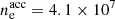(2009): B′₀ = 2000 G, $t{\prime }_{\mathrm{dyn}}=80$ s, $n_{\mathrm{e}}^{\mathrm{acc}}=4.1\times {10}^7$ cm⁻³, Γ_m = 1600, and p = 2.5 (see their Fig. 6). This led to Γ_c, 0/Γ_m = 1.5 × 10⁻³ (fast cooling). We then studied the effect on the spectrum of each physical parameter by varying its value while keeping all other parameters constant. We used the same radiative code as in Sects. 2.4 and 3 with a rapidly decaying magnetic field, but we included all processes (adiabatic cooling, synchrotron radiation and self-absorption, inverse Compton scattering, and photon-photon annihilation). The results are shown in Fig. 4 (effect of γ_m), Fig. 5 (effect of B′₀), Fig. 6 (effect of $t{\prime }_{\mathrm{dyn}}$), and Fig. 7 (effect of $n_{\mathrm{e}}^{\mathrm{acc}}$) for a constant magnetic field (left panels in the figures) and for a decaying magnetic field with $t{\prime }_{\mathrm{B}}/t{\prime }_{\mathrm{dyn}}={10}^{-3}$ (right panels). The panels with a constant magnetic field just reproduce the results in Fig. 6 of Bošnjak et al. (2009) for an easier comparison with the decaying case discussed here. As expected, the magnetic field decay leads to a clear increase of the low-energy photon index of the synchrotron component in most cases. In the following, we describe the effect of each physical parameter.

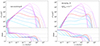Fig. 4. Emission in the co-moving frame: Effect of the electron Lorentz factor. Starting from the reference case shown in red (Γm = 1600, B′0 = 2000 G, ne, acc = 4.1 × 107 cm−3, tdyn = 80 s), we plot the evolution of the spectrum when varying the electron Lorentz factor, either assuming a constant (left) or a decaying (right) magnetic field. The adopted values are Γm = 51 (cyan), 160, 510, 1600, 5100, 1.6 × 104, 5 × 104, and 1.6 × 105 (magenta). The spectra obtained when pair production and synchrotron self-absorption are not included are shown with thin lines. Dashed lines show the spectra that do not satisfy the conditions for transparency (τT < 0.1) or that are radiatively inefficient (frad < 50%).

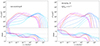Fig. 5. Emission in the co-moving frame: Effect of the magnetic field. Same as in Fig. 4 but now varying the initial magnetic field. The adopted values are B′0 [G] = 6 (cyan), 20, 63, 200, 632, 2000, 2 × 104, and 2 × 105 (magenta).

Effect of the electron minimum Lorentz factor (Fig. 4). The peak energy of the synchrotron spectrum increases with Γ_m. Compared to the standard case, the magnetic field decay has two effects: (i) As expected, the low-energy photon index increases due to a larger effective critical Lorentz factor, 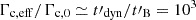${\mathrm{\Gamma }}_{\mathrm{c},\mathrm{eff}}/{\mathrm{\Gamma }}_{\mathrm{c},0}\simeq t{\prime }_{\mathrm{dyn}}/t{\prime }_{\mathrm{B}}={10}^3$ (see the steepening of the νu_ν spectrum at low frequency in the top-right panel). (ii) In addition, the intensity of the inverse Compton component is increased. This is due to a longer synchrotron timescale. The effect is stronger for low values of Γ_m, as the Klein-Nishina regime strongly limits the inverse Compton scatterings for higher synchrotron peak energies. Dashed lines in the figure indicate the limits of the regime of interest. The radiative efficiency becomes too low for a small electron Lorentz factor (slow cooling), and the optically thin assumption is not valid anymore for a very large electron Lorentz factor due to the production of pairs by high-energy photons.

Effect of the magnetic field (Fig. 5). When B′₀ decreases, the efficiency of inverse Compton scatterings increases – lower Compton parameter, Eq. (12) – but the peak energy of the synchrotron spectrum also decreases so that the lowest values of B′₀ correspond to a low radiative efficiency (slow cooling, dashed lines). The inverse Compton component is dominant in this case (Thomson regime), which is unlikely in GRB spectra (Bošnjak et al. 2009; Piran et al. 2009). For higher values of the magnetic field, the Klein-Nishina regime limits the intensity of the inverse Compton component at high-energy but contributes to the steepening of the low-energy synchrotron slope in the νu_ν spectrum (Nakar et al. 2009; Bošnjak et al. 2009; Daigne et al. 2011). Compared to the standard case, the magnetic field decay has two effects: (i) an expected increase of the low-energy photon index in the synchrotron component and (ii) an increased intensity of the high-energy inverse Compton component due to a lower effective magnetic field energy density.

Effect of the dynamical timescale (Fig. 6). The dynamical timescale directly impacts the critical Lorentz factor Γ_c, 0 (Eq. 2) and therefore also the radiative regime of electrons. To avoid a low radiative efficiency, electrons should be in fast cooling, which constrains $t{\prime }_{\mathrm{dyn}}$ as being greater than the synchrotron timescale $t{\prime }_{\mathrm{syn}}({\mathrm{\Gamma }}_{\mathrm{m}})$, equal to 0.12 s in the reference case. The lowest values of $t{\prime }_{\mathrm{dyn}}$ in the left panel of Fig. 6 therefore correspond to marginally fast cooling with an increase of the low-energy photon index. Compared to the standard case, the magnetic field decay again leads to the two expected effects: (i) The marginally fast cooling regime is more easily reached, with a clear increase of the low-energy photon index. This effect disappears for the largest values of $t{\prime }_{\mathrm{dyn}}$, as $\mathrm{\Gamma }{\prime }_{\mathrm{c},0}$ becomes very small. (ii) The intensity of the inverse Compton component at high energy is enhanced. The regime of interest remains limited by the condition on the radiative efficiency (f_rad ≳ 50% for $t{\prime }_{\mathrm{dyn}}\gtrsim 1$ s) and by the increasing opacity due to secondary pairs (optically thick regime for $t{\prime }_{\mathrm{dyn}}\gtrsim 8000$ s).

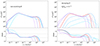Fig. 6. Emission in the co-moving frame: Effect of the dynamical timescale. Same as in Fig. 4 but now varying the dynamical timescale. The adopted values are tdyn [s] = 0.08 (cyan), 0.8, 8, 80, 800, and 8 × 103 (magenta).

Effect of the density of accelerated electrons (Fig. 7). The intensity of the inverse Compton component at high energy increases with the electron density (Eq. 12), but it saturates for the highest densities because of the pair production. The magnetic field decay has a similar effect at all densities, with a clear increase of the low-energy photon index of the synchrotron component.

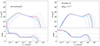Fig. 7. Emission in the co-moving frame: Effect of the electron density. Same as in Fig. 4 but now varying the electron density. The adopted values are ne, acc [cm−3] = 4.1 × 105 (cyan), 4.1 × 106, 4.1 × 107, 4.1 × 108, and 4.1 × 109 (magenta).

4.2. Consequences for the spectral evolution during the gamma-ray burst prompt emission

During the GRB prompt phase, there are several emission zones in the relativistic ejecta with possibly different physical conditions (that may evolve). Therefore, some spectral evolution is expected, in agreement with observations. In particular, studies of bright, isolated pulses have demonstrated that there are typical patterns occurring in prompt GRB spectral evolution, such as the hard-to-soft evolution of peak energy E_p with time, the correlation between intensity and the peak energy E_p, and the low-energy photon index α evolving with E_p (see e.g. Ford et al. 1995; Crider et al. 1997; Peng et al. 2009; Lu et al. 2012; Hakkila et al. 2015; Yu et al. 2016).

In the context of synchrotron radiation with a decaying magnetic field, we expected from the discussion in the previous subsection that both the peak energy and the low-energy spectral slope should evolve together with the physical properties in the emission region. In order to model this spectral evolution, a specific internal dissipation process must be assumed in the relativistic ejecta. This was done here in the context of the internal shock model, following the approach described in Bošnjak et al. (2009). The dynamics of a relativistic ejecta with a variable initial distribution of the Lorentz factor was computed using the ballistic approximation of Daigne & Mochkovitch (1998). For each internal shock forming and propagating in the ejecta, the radiation at each time step was computed with the same radiative code as before, including all relevant processes (adiabatic cooling, synchrotron radiation and self-absorption, inverse Compton scattering, photon-photon annihilation) and a rapidly decaying magnetic field. The observed light curves and spectra were then computed by a full integration over equal-arrival time surfaces, taking into account relativistic and cosmological effects.

4.2.1. Evolution of the physical conditions in internal shocks and associated spectral evolution

We modelled a typical pulse in a GRB gamma-ray light curve produced by the emission of electrons accelerated in internal shocks resulting from the collision of a fast region with a Lorentz factor Γ₂ and a slow region with a Lorentz factor Γ₁ < Γ₂. We studied the same references cases as Daigne et al. (2011) and Bošnjak & Daigne (2014): We considered an ejection lasting t_w = 2 s with a constant injected kinetic power $\dot{E}={10}^{54}$ erg/s and a Lorentz factor evolving from Γ₁ = 100 to Γ₂ = 400. We assumed that a fraction ϵ_e of the energy dissipated in internal shocks is injected into non-thermal electrons that represent a fraction ζ of all electrons and that a fraction ϵ_B of the dissipated energy is injected in an amplified magnetic field of intensity B′₀ in the acceleration site. The index of the power-law distribution of accelerated electrons is p = 2.5. Case (A) assumes ζ = 3 × 10⁻³ and ϵ_B = 1/3 (high magnetic field, very weak inverse Compton emission), and case (B) assumes ζ = 10⁻³ and ϵ_B = 10⁻³ (low magnetic field). In both cases, the synchrotron component is dominant and peaks in the gamma-ray range. Without any magnetic field decay, case (A) corresponds to the standard fast cooling synchrotron spectrum with E_p ≃ 700 keV and α = −3/2, and case (B) corresponds to a harder spectrum with E_p ≃ 800 keV and α ≃ −1 due to the effect of inverse Compton scatterings in the Klein-Nishina regime.

We show case (A) in Fig. 8 and case (B) in Fig. 9 when the effect of a decaying magnetic field is included, assuming $t{\prime }_{\mathrm{B}}/t{\prime }_{\mathrm{dyn}}={10}^{-4}$ in case (A) and 10⁻³ in case (B). Light curves in different energy channels (covering the spectral range of the Fermi/GBM and LAT instruments) are plotted in the left panels of the figures and the time-evolving spectrum is plotted in the right panels. In addition, the evolution of the parameters governing the synchrotron and inverse Compton regime, namely, Γ_c, 0/Γ_m, Y_Th, and w_m, are plotted in the top-left panels, and the photon index is plotted in the bottom-right panels. With our choice of timescales for the magnetic field decay, the condition given by Eq. (3) is fulfilled in both cases at the maximum of the pulse. As expected, the low-energy νF_ν spectrum is much steeper when including the magnetic field decay, with α ≃ −0.8 in both cases.

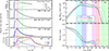Fig. 8. Effect of a decaying magnetic field in the internal shock model: Reference case A with $t{\prime }_{\mathrm{B}}/t{\prime }_{\mathrm{dyn}}={10}^{-4}$. Left: Light curves in the GBM and LAT range. The top panel shows the evolution of the parameters wm, YTh, and Γc, 0/Γm in the co-moving frame of the shocked material. Right: Spectra in the four time bins indicated on the light curves and corresponding to the rise, the peak, and the decay of the pulse.

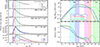Fig. 9. Effect of a decaying magnetic field in the internal shock model: Reference case B with $t{\prime }_{\mathrm{B}}/t{\prime }_{\mathrm{dyn}}={10}^{-3}$. Same as in Fig. 8.

In addition, we observed a clear spectral evolution during the pulse, with both the peak energy and the low-energy photon index evolving from the rise to the peak of the pulse, and then from the peak to the decay, with a general hard-to-soft trend. Finally, the inverse Compton emission becomes efficient even in case (A) during the decay phase, leading in both cases to a slightly delayed emission in the high-energy range above 1 GeV (see bottom-left panel in Figs. 8 and 9).

We note that all the microphysics parameters (ϵ_e, ζ, p, ϵ_B) were assumed to be constant. Any evolution with the shock conditions would affect the details of the observed spectral evolution, as discussed in Daigne & Mochkovitch (2003) and Bošnjak & Daigne (2014). In addition, the ratio $t{\prime }_{\mathrm{B}}/t{\prime }_{\mathrm{dyn}}$ has also been assumed to be constant for simplicity. We discuss this assumption in the next subsection.

4.2.2. Evolution of the timescale of the magnetic field decay

In the fast cooling regime, the electrons typically responsible for the peak and the low-energy part of the synchrotron spectrum cool and radiate on a timescale that is orders of magnitude above the plasma scale at their acceleration site but orders of magnitude below the dynamical timescale of the ejecta. Then, the electrons probe a magnetic field on a scale that is neither accessible to PIC simulations of the acceleration process (typically ∼10⁴ plasma scales at maximum; see e.g. Keshet et al. 2009; Crumley et al. 2019) nor to large-scale MHD simulations of the propagating ejecta (e.g. Bromberg & Tchekhovskoy 2016). Therefore, we do not have predictions for the realistic magnetic field structure to take into account for the synchrotron radiations in GRBs that could be compared to the very simple prescription used in this paper (exponential decay) and the condition given by Eq. (3) on the decay scale.

The spectral evolution shown in Figs. 8 and 9 was computed assuming a constant ratio $t{\prime }_{\mathrm{B}}/t{\prime }_{\mathrm{dyn}}$, that is, a strong correlation between the magnetic field decay timescale and the dynamical timescale of the ejecta. Another possible assumption would be to consider a strong correlation between the decay scale and the plasma scale, such as a constant ratio $t{\prime }_{\mathrm{B}}/t{\prime }_{\mathrm{pl}}$, where $ct{\prime }_{\mathrm{pl}}$ is the plasma electron skin depth, given by (see e.g. Pe’er & Zhang 2006):

$$\begin{array}{c}\hfill t_{\mathrm{pl}}^{\prime }=\frac{1}{{\omega }_{\mathrm{pl},\mathrm{e}}^{\prime }}=\sqrt{\frac{{\gamma }_{\mathrm{m}}{m}_e}{4\pi e^2{n}_{\mathrm{e}}^{\prime }}},\end{array}$$(16)

where $n{\prime }_{\mathrm{e}}=n{\prime }_{\mathrm{p}}$ is the co-moving density. In agreement with Eq. (3), Pe’er & Zhang (2006) found that hard synchrotron spectrum in GRBs could be expected for $t{\prime }_{\mathrm{B}}/t{\prime }_{\mathrm{pl}}\sim {10}^5$. If we assume a constant ratio $t{\prime }_{\mathrm{B}}/t{\prime }_{\mathrm{pl}}$, the spectral evolution should be affected, as the ratio $t{\prime }_{\mathrm{B}}/t{\prime }_{\mathrm{dyn}}$ then evolves. For the two cases shown in Figs. 8 and 9, we plot in Fig. 10 the evolution of the physical conditions in the emission region in the $t{\prime }_{\mathrm{B}}/t{\prime }_{\mathrm{dyn}}$ versus Γ_c, 0/Γ_m plane relevant for understanding the regime of the synchrotron emission. This evolution is plotted for $t{\prime }_{\mathrm{B}}/t{\prime }_{\mathrm{pl}}={10}^6$, 10⁷, and 10⁸, which are intermediate values between the estimates considered by Pe’er & Zhang (2006) (∼10⁵) and Piran (2005) (∼10⁹). This high ratio confirms that we probe here the evolution of the magnetic field on a scale that is much larger than the plasma scale³ at the acceleration site. For comparison, lines of constant low-energy photon index, α = −1.5, −1.25, −1 and −0.75, are also plotted, assuming Y_Th, 0 = 0.1 and w_m = 10² in case A and Y_Th, 0 = 10² and w_m = 10² in case B, which are representative of the conditions close to the peak of the pulse (see top-left panels in Figs. 8 and 9). A red cross indicates the time where the dissipated energy per unit mass is maximum. Compared to a constant ratio $t{\prime }_{\mathrm{B}}/t{\prime }_{\mathrm{dyn}}$, which would correspond to a horizontal line in Fig. 10, we find that a correlation with the plasma scale leads to an evolution of $t{\prime }_{\mathrm{B}}/t{\prime }_{\mathrm{dyn}}$, which allows the synchrotron radiation to stay for most of the pulse in the regime with the hardest low-energy spectral slope. This comparison could be improved by taking into account the evolution of w_m (and possibly Y_Th, 0 if other microphysics parameters such as ϵ_B are also varying). Other evolutions between these two extreme cases are possible. For instance, the intrinsic pair loading mechanism proposed by Derishev & Piran (2016) leads to a strong correlation between $t{\prime }_{\mathrm{B}}$ and the radiative timescale of electrons.

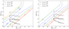Fig. 10. Evolution of $t{\prime }_B/t{\prime }_{\mathrm{dyn}}$ and Γc, 0/Γm during the pulse duration. Left: Evolution for case A. The contour lines for values of α = −1.5, −1.25, −1, −0.75 are shown, using the simulations obtained for YTh, 0 = 0.1; wm = 102 (adopted from the upper right plot of Fig. 3). Right: Evolution for case B. The same contour lines are shown for α, using the simulations obtained for YTh, 0 = 102; wm = 102 (adopted from the middle-left plot of Fig. 3). We have overplotted (in grey lines) the values of $t_{\mathrm{B}}\prime /t_{\mathrm{dyn}}\prime$ calculated using the parameters of the dynamical evolution (Γm and density in the co-moving frame) for case (A) and case (B) and assuming a constant ratio $t{\prime }_{\mathrm{B}}/t{\prime }_{\mathrm{pl}}={10}^6$, 107, or 108. Red crosses show values at the maximum of the pulse, that is, where the dissipated energy per unit mass obtains maximum.

We conclude that if the prompt GRB emission is produced by synchrotron radiation, the observed spectral evolution is most probably strongly affected by the unknown structure of the magnetic field at intermediate scales, but we do not pursue this exploration further due to the absence of a realistic prescription.

5. Discussion and conclusions

If the prompt GRB emission is dominated by synchrotron radiation from electrons accelerated by internal shocks or reconnection above the photosphere, they must be in the fast cooling regime to explain the huge luminosities observed and the high variability. Therefore, their radiative timescale is much shorter than the dynamical timescale $t{\prime }_{\mathrm{dyn}}$ of the ejecta, but it is also much longer than the plasma scale $t{\prime }_{\mathrm{pl}}$ at the acceleration site. We have explored the effect of a possible evolution of the magnetic field on the emitted spectrum at such intermediate scales, which cannot currently be probed by large-scale MHD simulations or by PIC simulations. In the absence of any available prediction for the evolution of the magnetic field at these scales, we have adopted a simple prescription with an exponential decay on a timescale $t{\prime }_{\mathrm{B}}$, with $t{\prime }_{\mathrm{pl}}\ll t{\prime }_{\mathrm{B}}\ll t{\prime }_{\mathrm{dyn}}$. Our detailed calculations, which include not only the synchrotron radiation but also a detailed treatment of inverse Compton scatterings with Klein-Nishina corrections as well as synchrotron self-absorption at low energy and pair production at high energy, show that such a decaying magnetic field has a strong impact on the emission, with a significant steepening of the low-energy part of the νF_ν spectrum. The effect leads to three main results:

(1) Low-energy photon index α in the soft gamma-ray range. A possible rapid magnetic field decay is a natural mechanism to reach the marginally fast cooling regime (Daigne et al. 2011; Beniamini & Piran 2013), with α close to −2/3 while maintaining a high radiative efficiency. The highest values of the low-energy photon index, α ≃ −2/3, were obtained in a broad region of the parameter space where the magnetic field decays on an intermediate timescale between the radiative timescale of electrons at Γ_m and the dynamical timescale $t{\prime }_{\mathrm{dyn}}$. Precisely, our numerical results show that the approximate condition for this marginal fast cooling regime is $0.1{\mathrm{\Gamma }}_{\mathrm{c},0}/{\mathrm{\Gamma }}_{\mathrm{m}}\lesssim t{\prime }_{\mathrm{B}}/t{\prime }_{\mathrm{dyn}}\lesssim 10{\mathrm{\Gamma }}_{\mathrm{c},0}/{\mathrm{\Gamma }}_{\mathrm{m}}$. This corresponds to a characteristic scale of the magnetic field decay that is typically around seven to eight orders of magnitude above the plasma skin depth at the acceleration site, which is in agreement with the results of previous studies (Piran 2005; Pe’er & Zhang 2006). For a slower magnetic field decay, $10{\mathrm{\Gamma }}_{\mathrm{c},0}/{\mathrm{\Gamma }}_{\mathrm{m}}\lesssim t{\prime }_{\mathrm{B}}/t{\prime }_{\mathrm{dyn}}$, its effect is much weaker. The low-energy photon index is then in the range −3/2 ≤ α ≲ −1, depending on the importance of inverse Compton scatterings in the Klein-Nishina regime. On the other hand, a much faster decay ($t{\prime }_{\mathrm{B}}/t{\prime }_{\mathrm{dyn}}\lesssim 0.1{\mathrm{\Gamma }}_{\mathrm{c},0}/{\mathrm{\Gamma }}_{\mathrm{m}}$) can lead to much flatter spectra (−2 < α < −3/2), as the whole electron population enters the slow cooling regime. This leads to a low radiative efficiency. However, a non-negligible background magnetic field may very well dominate the electron evolution in this specific regime (Zhou et al. 2023). We have shown that by varying the physical conditions in the emission region (electron Lorentz factor at injection, magnetic field, electron density, dynamical timescale), all of these different regimes of the synchrotron fast cooling can be explored.

(2) Spectral evolution. During the GRB prompt emission, synchrotron radiation is expected from accelerated electrons in different emission zones (e.g. shocks or reconnection sites), which leads to the observed diversity and variability of GRB light curves. In addition, the physical conditions in each emission zone can evolve, which naturally leads to some spectral evolution, even within a single pulse. Such a spectral evolution is observed in the time-resolved spectral analysis of bright GRBs (see e.g. Yu et al. 2016). We have shown some examples of the spectral evolution expected in the case of a pulse produced by an internal shock in Sect. 4.2: The peak energy and the low-energy photon index vary significantly during the rise and the decay of the pulse light curve. However, the predicted evolution depends strongly on the assumed prescription for the characteristic scale of the magnetic decay. This prescription is very uncertain in the absence of simulations covering the full range of scales from the plasma scale at the acceleration site to the geometrical width of the ejecta. The results shown here are limited to the specific case where $t{\prime }_{\mathrm{B}}$ is strongly correlated to the dynamical timescale $t{\prime }_{\mathrm{dyn}}$.

(3) High-energy emission. The Fermi/LAT observations show some diversity regarding the prompt high-energy emission (Ajello et al. 2019): The ratio between the fluences in the 0.1−100 GeV and 10 keV−1 MeV channels ranges from ∼10⁻² to ∼1 for the cases with a LAT detection (during the GBM time window). The synchrotron self-Compton component in the Klein-Nishina regime is a natural candidate to explain this behaviour (Bošnjak et al. 2009). We have shown here that it is also affected by a possible magnetic field decay in the emission zone. Indeed, the effective Compton parameter increases with time as the magnetic field decays. As discussed in Sect. 3, our exploration of the parameter space shows ratios of the intensity of these two components L_ic/L_syn ranging from very low values when the Klein-Nishina reduction is strong to larger values of the order of L_ic/L_syn ≃ 0.1 − 1, which is in agreement with the observed diversity of the prompt high-energy component.

Our main conclusion is that efficient synchrotron radiation in a rapidly decaying magnetic field can reproduce low-energy photon indices ranging from α = −3/2 to −2/3, in agreement with the measured value in the majority of GRBs (see e.g. Goldstein et al. 2013; Gruber et al. 2014; Poolakkil et al. 2021). For instance, the peak spectrum of the GRBs in the best sample of the Fermi/GBM spectral catalogue shows α < −2/3 in about 78% of cases, with a median value and 68% confidence level interval $\alpha =-1.{30}_{-0.33}^{+0.77}$ (Poolakkil et al. 2021), and the time-resolved spectral analysis of the brightest Fermi/GBM over the four first years shows a median value of $\alpha =-0.{77}_{-0.32}^{+0.27}$ (Yu et al. 2016). We note that the measured value of α is affected by the imposed shape of the phenomenological function used for the spectral fit, usually the Band function (Band et al. 1993). Oganesyan et al. (2017), Ravasio et al. (2018), Toffano et al. (2021), Poolakkil et al. (2023) have obtained good spectral fits to several bright GRBs by adding a second break in the spectrum, often close to the peak energy, with low-energy photon indices close to −2/3 and −3/2, which is reminiscent of the marginally fast cooling regime naturally favoured by the magnetic field decay described here. However, we also note that the theoretical synchrotron spectral shape cannot be directly compared to data, as it should be convoluted with the evolution of the physical conditions in the emission zone, which tends to smooth and broaden the spectral breaks, as illustrated in the simulations shown in Sect. 4.2 in the context of the internal shock model (see also Yan et al. 2024). Yassine et al. (2020) introduced the “internal shock synchrotron model” (ISSM) phenomenological function with four free parameters, which has a smoothly evolving photon index all along the soft gamma-ray range and fits well synthetic spectra produced by fast cooling synchrotron radiation in internal shocks. They find that the ISSM can usually fit the spectra of a sample of 74 bright Fermi/GBM bursts at least as well as the Band function, with a low-energy photon index α < −2/3 in 74% of cases. Finally, we note that in all scenarios for the prompt emission where soft gamma rays are produced by synchrotron radiation in the optically thin region, a weak quasi-thermal photospheric emission is also expected (see e.g. Hascoët et al. 2013). Guiriec et al. (2015 2017), Li (2019) have shown that adding a weak thermal component in the spectral fit can also significantly affect the measured value of the low-energy photon index α of the non-thermal component, usually by decreasing it.

For better comparison in the future, it will be necessary to be able to perform the spectral analysis of GRB data directly using a detailed synchrotron model, as described in this paper, coupled with a dynamical calculation of the relativistic ejecta and probably also including the contribution of the photospheric emission. This goes far beyond the scope of the present paper and seems difficult to achieve in the short term. On the other hand, there are good short-term prospects for a better measurement of the prompt GRB spectrum, especially in the low-energy index α, thanks to the Space-based multi-band astronomical Variable Objects Monitor mission launched on 22 June 2024 (Wei et al. 2016), which uses a low-energy threshold at 4 keV of the coded-mask telescope ECLAIRs with a spectral range extending to 5 MeV for the Gamma-Ray Monitor (Bernardini et al. 2017).

Acknowledgments

The authors thank Robert Mochkovitch, Frédéric Piron and Martin Lemoine for fruitful discussions about this study. The research leading to these results has received funding (Ž.B.) from the European Union’s Horizon 2020 Programme under the AHEAD2020 project (grant agreement n. 871158). F.D. acknowledges the Centre National d’Études Spatiales (CNES) for financial support in this research project.

References

All Figures

Fig. 1. Effect of a decaying magnetic field on the synchrotron spectrum. The normalised spectrum ν′uν′/ue is plotted as a function of the normalised frequency $\nu \prime /\nu {\prime }_{\mathrm{m}}$ for a constant magnetic field (dotted line) or a decaying magnetic field on a timescale $t{\prime }_{\mathrm{B}}={10}^{-2}t{\prime }_{\mathrm{dyn}}$ (solid line). The calculation has been done with the numerical radiative code described in Sect. 2.4 either including only the synchrotron process (black) or both the synchrotron radiation and the inverse Compton scatterings (red). The following parameters were adopted: Γc, 0 = Γm/300, YTh = 10, wm = 102, and p = 2.5. In the synchrotron-only case, the result of the approximate calculation discussed in Sect. 2.3 is plotted in blue for comparison.

In the text

Fig. 2. Effect of a decaying magnetic field on the synchrotron spectrum: Realistic case including inverse Compton scatterings. The normalised synchrotron spectrum νuν/ue as well as the photon index are plotted as a function of the normalised frequency $\nu \prime /\nu {\prime }_{\mathrm{m}}$ for a constant magnetic field (black) or a decaying magnetic field on a timescale of $t{\prime }_{\mathrm{B}}/t{\prime }_{\mathrm{dyn}}={10}^{-1}$ (red) and 10−2 (blue). The calculation includes adiabatic cooling, synchrotron radiation, and inverse Compton scatterings but does not take into account synchrotron self-absorption and pair production. Each panel corresponds to a different value of the parameter wm, which measures the importance of Klein-Nishina effects, from 10−2 (Thomson regime) to 104 (strong Klein-Nishina regime). The spectra are plotted for YTh = 10−1, 1, 10, 102, 103, and 104, which corresponds to an increasing efficiency of scatterings (see text). We assumed everywhere an electron slope p = 2.5 and a magnetic field B′0 in the acceleration site corresponding to Γc/Γm = 1/300.

In the text

Fig. 3. Synchrotron emission within a decaying magnetic field: Parameter space. In the $t{\prime }_{\mathrm{B}}/t{\prime }_{\mathrm{dyn}}$ vs Γc, 0/Γm plane, the value of the low-energy photon index α of the synchrotron spectrum is colour-coded. In this plane, the standard synchrotron spectrum with a constant magnetic field is at the top ($t{\prime }_{\mathrm{B}}\to \infty$). In this case the fast cooling regime is on the left (Γc, 0 ≪ Γm), while the marginally fast cooling regime is on the right (Γc, 0 ≃ Γm). Black solid lines indicate the limits of the high radiative efficiency region (thick: frad = 0.9; thin: frad = 0.5; very thin: fdad = 0.1). Contours of the inverse Compton/synchrotron ratio Lic/Lsyn are plotted with black dashed lines. Each panel corresponds to a set of values for the parameters YTh, 0 and wm that govern the importance of inverse Compton scatterings and Klein-Nishina corrections. (a) YTh, 0 = 0.1; wm = 10−2. (b) YTh, 0 = 0.1; wm = 102. (c) YTh, 0 = 102; wm = 102. (d) YTh, 0 = 102; wm = 104. (e) YTh, 0 = 104; wm = 104.

In the text

Fig. 4. Emission in the co-moving frame: Effect of the electron Lorentz factor. Starting from the reference case shown in red (Γm = 1600, B′0 = 2000 G, ne, acc = 4.1 × 107 cm−3, tdyn = 80 s), we plot the evolution of the spectrum when varying the electron Lorentz factor, either assuming a constant (left) or a decaying (right) magnetic field. The adopted values are Γm = 51 (cyan), 160, 510, 1600, 5100, 1.6 × 104, 5 × 104, and 1.6 × 105 (magenta). The spectra obtained when pair production and synchrotron self-absorption are not included are shown with thin lines. Dashed lines show the spectra that do not satisfy the conditions for transparency (τT < 0.1) or that are radiatively inefficient (frad < 50%).

In the text

	Fig. 5. Emission in the co-moving frame: Effect of the magnetic field. Same as in Fig. 4 but now varying the initial magnetic field. The adopted values are B′0 [G] = 6 (cyan), 20, 63, 200, 632, 2000, 2 × 104, and 2 × 105 (magenta).
In the text

	Fig. 6. Emission in the co-moving frame: Effect of the dynamical timescale. Same as in Fig. 4 but now varying the dynamical timescale. The adopted values are tdyn [s] = 0.08 (cyan), 0.8, 8, 80, 800, and 8 × 103 (magenta).
In the text

	Fig. 7. Emission in the co-moving frame: Effect of the electron density. Same as in Fig. 4 but now varying the electron density. The adopted values are ne, acc [cm−3] = 4.1 × 105 (cyan), 4.1 × 106, 4.1 × 107, 4.1 × 108, and 4.1 × 109 (magenta).
In the text

Fig. 8. Effect of a decaying magnetic field in the internal shock model: Reference case A with $t{\prime }_{\mathrm{B}}/t{\prime }_{\mathrm{dyn}}={10}^{-4}$. Left: Light curves in the GBM and LAT range. The top panel shows the evolution of the parameters wm, YTh, and Γc, 0/Γm in the co-moving frame of the shocked material. Right: Spectra in the four time bins indicated on the light curves and corresponding to the rise, the peak, and the decay of the pulse.

In the text

	Fig. 9. Effect of a decaying magnetic field in the internal shock model: Reference case B with $t{\prime }_{\mathrm{B}}/t{\prime }_{\mathrm{dyn}}={10}^{-3}$. Same as in Fig. 8.
In the text

Fig. 10. Evolution of $t{\prime }_B/t{\prime }_{\mathrm{dyn}}$ and Γc, 0/Γm during the pulse duration. Left: Evolution for case A. The contour lines for values of α = −1.5, −1.25, −1, −0.75 are shown, using the simulations obtained for YTh, 0 = 0.1; wm = 102 (adopted from the upper right plot of Fig. 3). Right: Evolution for case B. The same contour lines are shown for α, using the simulations obtained for YTh, 0 = 102; wm = 102 (adopted from the middle-left plot of Fig. 3). We have overplotted (in grey lines) the values of $t_{\mathrm{B}}\prime /t_{\mathrm{dyn}}\prime$ calculated using the parameters of the dynamical evolution (Γm and density in the co-moving frame) for case (A) and case (B) and assuming a constant ratio $t{\prime }_{\mathrm{B}}/t{\prime }_{\mathrm{pl}}={10}^6$, 107, or 108. Red crosses show values at the maximum of the pulse, that is, where the dissipated energy per unit mass obtains maximum.

In the text

References

- Abdalla, H., Adam, R., Aharonian, F., et al. 2019, Nature, 575, 464 [Google Scholar]
- Ackermann, M., Ajello, M., Asano, K., et al. 2011, ApJ, 729, 114 [CrossRef] [Google Scholar]
- Ackermann, M., Ajello, M., Asano, K., et al. 2013, ApJS, 209, 11 [NASA ADS] [CrossRef] [Google Scholar]
- Acuner, Z., Ryde, F., Pe’er, A., Mortlock, D., & Ahlgren, B. 2020, ApJ, 893, 128 [NASA ADS] [CrossRef] [Google Scholar]
- Ajello, M., Arimoto, M., Axelsson, M., et al. 2019, ApJ, 878, 52 [NASA ADS] [CrossRef] [Google Scholar]
- Band, D., Matteson, J., Ford, L., et al. 1993, ApJ, 413, 281 [Google Scholar]
- Barniol Duran, R., Bošnjak, Ž., & Kumar, P. 2012, MNRAS, 424, 3192 [CrossRef] [Google Scholar]
- Beloborodov, A. M. 2010, MNRAS, 407, 1033 [NASA ADS] [CrossRef] [Google Scholar]
- Beniamini, P., & Piran, T. 2013, ApJ, 769, 69 [Google Scholar]
- Bernardini, M. G., Xie, F., Sizun, P., et al. 2017, Exp. Astron., 44, 113 [NASA ADS] [CrossRef] [Google Scholar]
- Bošnjak, Ž., & Daigne, F. 2014, A&A, 568, A45 [NASA ADS] [CrossRef] [EDP Sciences] [Google Scholar]
- Bošnjak, Ž., Daigne, F., & Dubus, G. 2009, A&A, 498, 677 [NASA ADS] [CrossRef] [EDP Sciences] [Google Scholar]
- Bromberg, O., & Tchekhovskoy, A. 2016, MNRAS, 456, 1739 [CrossRef] [Google Scholar]
- Bykov, A., Romansky, V., & Osipov, S. 2022, Universe, 8, 32 [NASA ADS] [CrossRef] [Google Scholar]
- Chang, P., Spitkovsky, A., & Arons, J. 2008, ApJ, 674, 378 [NASA ADS] [CrossRef] [Google Scholar]
- Cherenkov Telescope Array Consortium (Acharya, B. S., et al.) 2019, Science with the Cherenkov Telescope Array (World Scientific Publishing) [Google Scholar]
- Cohen, E., Katz, J. I., Piran, T., et al. 1997, ApJ, 488, 330 [NASA ADS] [CrossRef] [Google Scholar]
- Crider, A., Liang, E. P., Smith, I. A., et al. 1997, ApJ, 479, L39 [NASA ADS] [CrossRef] [Google Scholar]
- Crumley, P., Caprioli, D., Markoff, S., & Spitkovsky, A. 2019, MNRAS, 485, 5105 [NASA ADS] [CrossRef] [Google Scholar]
- Daigne, F., & Mochkovitch, R. 1998, MNRAS, 296, 275 [NASA ADS] [CrossRef] [Google Scholar]
- Daigne, F., & Mochkovitch, R. 2002, MNRAS, 336, 1271 [NASA ADS] [CrossRef] [Google Scholar]
- Daigne, F., & Mochkovitch, R. 2003, MNRAS, 342, 587 [NASA ADS] [CrossRef] [Google Scholar]
- Daigne, F., Bošnjak, Ž., & Dubus, G. 2011, A&A, 526, A110 [NASA ADS] [CrossRef] [EDP Sciences] [Google Scholar]
- Derishev, E. V. 2007, Ap&SS, 309, 157 [NASA ADS] [CrossRef] [Google Scholar]
- Derishev, E. V., & Piran, T. 2016, MNRAS, 460, 2036 [NASA ADS] [CrossRef] [Google Scholar]
- Derishev, E. V., Kocharovsky, V. V., & Kocharovsky, V. V. 2001, A&A, 372, 1071 [NASA ADS] [CrossRef] [EDP Sciences] [Google Scholar]
- Drake, J. F., Swisdak, M., Che, H., & Shay, M. A. 2006, Nature, 443, 553 [Google Scholar]
- Drenkhahn, G., & Spruit, H. C. 2002, A&A, 391, 1141 [NASA ADS] [CrossRef] [EDP Sciences] [Google Scholar]
- Ford, L. A., Band, D. L., Matteson, J. L., et al. 1995, ApJ, 439, 307 [NASA ADS] [CrossRef] [Google Scholar]
- Geng, J.-J., Huang, Y.-F., Wu, X.-F., Zhang, B., & Zong, H.-S. 2018, ApJS, 234, 3 [Google Scholar]
- Ghisellini, G., Celotti, A., & Lazzati, D. 2000, MNRAS, 313, L1 [NASA ADS] [CrossRef] [Google Scholar]
- Giannios, D. 2008, A&A, 480, 305 [NASA ADS] [CrossRef] [EDP Sciences] [Google Scholar]
- Giannios, D., & Spruit, H. C. 2007, A&A, 469, 1 [NASA ADS] [CrossRef] [EDP Sciences] [Google Scholar]
- Goldstein, A., Preece, R. D., Mallozzi, R. S., et al. 2013, ApJS, 208, 21 [Google Scholar]
- Gottlieb, O., Liska, M., Tchekhovskoy, A., et al. 2022, ApJ, 933, L9 [NASA ADS] [CrossRef] [Google Scholar]
- Granot, J., Komissarov, S. S., & Spitkovsky, A. 2011, MNRAS, 411, 1323 [NASA ADS] [CrossRef] [Google Scholar]
- Gruber, D., Goldstein, A., Weller von Ahlefeld, V., et al. 2014, ApJS, 211, 12 [Google Scholar]
- Guiriec, S., Mochkovitch, R., Piran, T., et al. 2015, ApJ, 814, 10 [NASA ADS] [CrossRef] [Google Scholar]
- Guiriec, S., Gehrels, N., McEnery, J., Kouveliotou, C., & Hartmann, D. H. 2017, ApJ, 846, 138 [NASA ADS] [CrossRef] [Google Scholar]
- Hakkila, J., Lien, A., Sakamoto, T., et al. 2015, ApJ, 815, 134 [NASA ADS] [CrossRef] [Google Scholar]
- Hascoët, R., Daigne, F., & Mochkovitch, R. 2013, A&A, 551, A124 [NASA ADS] [CrossRef] [EDP Sciences] [Google Scholar]
- Keshet, U., Katz, B., Spitkovsky, A., & Waxman, E. 2009, ApJ, 693, L127 [NASA ADS] [CrossRef] [Google Scholar]
- Kobayashi, S., Piran, T., & Sari, R. 1997, ApJ, 490, 92 [Google Scholar]
- Kumar, P., Hernández, R. A., Bošnjak, Ž., & Barniol Duran, R. 2012, MNRAS, 427, L40 [NASA ADS] [Google Scholar]
- Lemoine, M. 2013, MNRAS, 428, 845 [NASA ADS] [CrossRef] [Google Scholar]
- Lemoine, M., Li, Z., & Wang, X.-Y. 2013, MNRAS, 435, 3009 [NASA ADS] [CrossRef] [Google Scholar]
- Lemoine, M., Gremillet, L., Pelletier, G., & Vanthieghem, A. 2019, Phys. Rev. Lett., 123, 035101 [CrossRef] [Google Scholar]
- LHAASO Collaboration 2023, Science, 380, 1390 [NASA ADS] [CrossRef] [Google Scholar]
- Li, L. 2019, ApJS, 245, 7 [NASA ADS] [CrossRef] [Google Scholar]
- Lu, R.-J., Wei, J.-J., Liang, E.-W., et al. 2012, ApJ, 756, 112 [Google Scholar]
- MAGIC Collaboration (Acciari, V. A., et al.) 2019, Nature, 575, 455 [Google Scholar]
- Marcowith, A., Ferrand, G., Grech, M., et al. 2020, Liv. Rev. Comput. Astrophys., 6, 1 [Google Scholar]
- McKinney, J. C., & Uzdensky, D. A. 2012, MNRAS, 419, 573 [Google Scholar]
- Medvedev, M. V., Fiore, M., Fonseca, R. A., Silva, L. O., & Mori, W. B. 2005, ApJ, 618, L75 [NASA ADS] [CrossRef] [Google Scholar]
- Nakar, E., Ando, S., & Sari, R. 2009, ApJ, 703, 675 [NASA ADS] [CrossRef] [Google Scholar]
- Oganesyan, G., Nava, L., Ghirlanda, G., & Celotti, A. 2017, ApJ, 846, 137 [Google Scholar]
- Panaitescu, A. 2019, ApJ, 886, 106 [NASA ADS] [CrossRef] [Google Scholar]
- Pe’er, A. 2008, ApJ, 682, 463 [NASA ADS] [CrossRef] [Google Scholar]
- Pe’er, A., & Zhang, B. 2006, ApJ, 653, 454 [NASA ADS] [CrossRef] [Google Scholar]
- Peng, Z. Y., Ma, L., Zhao, X. H., et al. 2009, ApJ, 698, 417 [NASA ADS] [CrossRef] [Google Scholar]
- Piran, T. 2005, AIP Conf. Ser., 784, 164 [NASA ADS] [CrossRef] [Google Scholar]
- Piran, T., Sari, R., & Zou, Y.-C. 2009, MNRAS, 393, 1107 [NASA ADS] [CrossRef] [Google Scholar]
- Poolakkil, S., Preece, R., Fletcher, C., et al. 2021, ApJ, 913, 60 [NASA ADS] [CrossRef] [Google Scholar]
- Poolakkil, S., Preece, R., & Veres, P. 2023, ApJ, 959, 91 [NASA ADS] [CrossRef] [Google Scholar]
- Preece, R. D., Briggs, M. S., Mallozzi, R. S., et al. 1998, ApJ, 506, L23 [Google Scholar]
- Ravasio, M. E., Oganesyan, G., Ghirlanda, G., et al. 2018, A&A, 613, A16 [NASA ADS] [CrossRef] [EDP Sciences] [Google Scholar]
- Rees, M. J., & Meszaros, P. 1994, ApJ, 430, L93 [Google Scholar]
- Rees, M. J., & Mészáros, P. 2005, ApJ, 628, 847 [NASA ADS] [CrossRef] [Google Scholar]
- Rossi, E., & Rees, M. J. 2003, MNRAS, 339, 881 [NASA ADS] [CrossRef] [Google Scholar]
- Ryde, F., Pe’er, A., Nymark, T., et al. 2011, MNRAS, 415, 3693 [NASA ADS] [CrossRef] [Google Scholar]
- Samuelsson, F., Lundman, C., & Ryde, F. 2022, ApJ, 925, 65 [NASA ADS] [CrossRef] [Google Scholar]
- Sari, R., & Piran, T. 1997, ApJ, 485, 270 [NASA ADS] [CrossRef] [Google Scholar]
- Sari, R., Narayan, R., & Piran, T. 1996, ApJ, 473, 204 [Google Scholar]
- Sari, R., Piran, T., & Narayan, R. 1998, ApJ, 497, L17 [Google Scholar]
- Silva, L. O., Fonseca, R. A., Tonge, J. W., et al. 2003, ApJ, 596, L121 [Google Scholar]
- Sironi, L., & Spitkovsky, A. 2014, ApJ, 783, L21 [NASA ADS] [CrossRef] [Google Scholar]
- Sironi, L., Spitkovsky, A., & Arons, J. 2013, ApJ, 771, 54 [Google Scholar]
- Spruit, H. C., Daigne, F., & Drenkhahn, G. 2001, A&A, 369, 694 [NASA ADS] [CrossRef] [EDP Sciences] [Google Scholar]
- Tchekhovskoy, A., McKinney, J. C., & Narayan, R. 2008, MNRAS, 388, 551 [NASA ADS] [CrossRef] [Google Scholar]
- Tchekhovskoy, A., Narayan, R., & McKinney, J. C. 2010, New Astron., 15, 749 [NASA ADS] [CrossRef] [Google Scholar]
- Thompson, C. 1994, MNRAS, 270, 480 [NASA ADS] [CrossRef] [Google Scholar]
- Toffano, M., Ghirlanda, G., Nava, L., et al. 2021, A&A, 652, A123 [NASA ADS] [CrossRef] [EDP Sciences] [Google Scholar]
- Uhm, Z. L., & Zhang, B. 2014, Nat. Phys., 10, 351 [Google Scholar]
- Vanthieghem, A., Lemoine, M., Plotnikov, I., et al. 2020, Galaxies, 8, 33 [NASA ADS] [CrossRef] [Google Scholar]
- Vurm, I., & Beloborodov, A. M. 2016, ApJ, 831, 175 [NASA ADS] [CrossRef] [Google Scholar]
- Wang, K., & Dai, Z.-G. 2021, Galaxies, 9, 68 [NASA ADS] [CrossRef] [Google Scholar]
- Wang, X.-Y., Li, Z., Dai, Z.-G., & Mészáros, P. 2009, ApJ, 698, L98 [NASA ADS] [CrossRef] [Google Scholar]
- Wei, J., Cordier, B., Antier, S., et al. 2016, ArXiv e-prints [arXiv:1610.06892] [Google Scholar]
- Yan, Z.-Y., Yang, J., Zhao, X.-H., Meng, Y.-Z., & Zhang, B.-B. 2024, ApJ, 962, 85 [NASA ADS] [CrossRef] [Google Scholar]
- Yang, J., Zhao, X.-H., Yan, Z., et al. 2023, ApJ, 947, L11 [NASA ADS] [CrossRef] [Google Scholar]
- Yassine, M., Piron, F., Mochkovitch, R., & Daigne, F. 2017, A&A, 606, A93 [NASA ADS] [CrossRef] [EDP Sciences] [Google Scholar]
- Yassine, M., Piron, F., Daigne, F., et al. 2020, A&A, 640, A91 [NASA ADS] [CrossRef] [EDP Sciences] [Google Scholar]
- Yu, H.-F., Preece, R. D., Greiner, J., et al. 2016, A&A, 588, A135 [NASA ADS] [CrossRef] [EDP Sciences] [Google Scholar]
- Zhang, B., & Yan, H. 2011, ApJ, 726, 90 [Google Scholar]
- Zhang, B.-B., Uhm, Z. L., Connaughton, V., Briggs, M. S., & Zhang, B. 2016, ApJ, 816, 72 [NASA ADS] [CrossRef] [Google Scholar]
- Zhao, X., Li, Z., Liu, X., et al. 2014, ApJ, 780, 12 [Google Scholar]
- Zhou, L., Lin, D.-B., Yang, X., et al. 2023, ApJ, 957, 109 [NASA ADS] [CrossRef] [Google Scholar]
- Zou, Y.-C., Piran, T., & Sari, R. 2009, ApJ, 692, L92 [NASA ADS] [CrossRef] [Google Scholar]