| Issue |
A&A
Volume 656, December 2021
|
|
|---|---|---|
| Article Number | A111 | |
| Number of page(s) | 24 | |
| Section | Stellar atmospheres | |
| DOI | https://doi.org/10.1051/0004-6361/202141563 | |
| Published online | 09 December 2021 | |
Corona and XUV emission modelling of the Sun and Sun-like stars
1
National Astronomical Observatory of Japan, National Institutes of Natural Sciences,
2-21-1 Osawa,
Mitaka,
Tokyo
181-8588,
Japan
e-mail: This email address is being protected from spambots. You need JavaScript enabled to view it.
2
Department of Earth and Space Science, Graduate School of Science, Osaka University,
Toyonaka,
Osaka
560-0043,
Japan
Received:
16
June
2021
Accepted:
6
September
2021
Abstract
The X-ray and extreme-ultraviolet (EUV) emissions from low-mass stars significantly affect the evolution of the planetary atmosphere. However, it is observationally difficult to constrain the stellar high-energy emission because of the strong interstellar extinction of EUV photons. In this study, we simulate the XUV (X-ray plus EUV) emission from Sun-like stars by extending the solar coronal heating model that self-consistently solves, with sufficiently high resolution, the surface-to-coronal energy transport, turbulent coronal heating, and coronal thermal response by conduction and radiation. The simulations are performed with a range of loop lengths and magnetic filling factors at the stellar surface. With the solar parameters, the model reproduces the observed solar XUV spectrum below the Lyman edge, thus validating its capability of predicting the XUV spectra of other Sun-like stars. The model also reproduces the observed nearly linear relation between the unsigned magnetic flux and the X-ray luminosity. From the simulation runs with various loop lengths and filling factors, we also find a scaling relation, namely log LEUV = 9.93 + 0.67 log LX, where LEUV and LX are the luminosity in the EUV (100 Å < λ ≤ 912 Å) and X-ray (5 Å < λ ≤ 100 Å) range, respectively, in cgs. By assuming a power–law relation between the Rossby number and the magnetic filling factor, we reproduce the renowned relation between the Rossby number and the X-ray luminosity. We also propose an analytical description of the energy injected into the corona, which, in combination with the conventional Rosner–Tucker–Vaiana scaling law, semi-analytically explains the simulation results. This study refines the concepts of solar and stellar coronal heating and derives a theoretical relation for estimating the hidden stellar EUV luminosity from X-ray observations.
Key words: Sun: corona / stars: coronae / X-rays: stars / ultraviolet: stars
© ESO 2021
1 Introduction
The Sun has an aura of hot plasma called the corona, which has a temperature of a few million kelvin (Edlén 1943). The image of the corona has been captured by the Atmospheric Imaging Assembly (Lemen et al. 2012) of NASA’s Solar Dynamics Observatory (Pesnell et al. 2012). The corona is not unique to the Sun and has been observed to surround low-mass main-sequence stars in general (Güdel et al. 1997). Due to its high temperature, the corona is the principal source of stellar XUV (X-ray plus EUV: extreme ultraviolet) emissions.
Stellar XUV emissions drive the expansion and thermal escape of planetary atmospheres (Vidal-Madjar et al. 2003; Lecavelier des Etangs et al. 2012; Owen & Wu 2013; Ehrenreich et al. 2015; Airapetian et al. 2017). Therefore, describing the stellar XUV emission in terms of the stellar fundamental parameters (luminosity, mass, radius, etc.) is essential in understanding the evolution of a planet and its habitability. Since stellar XUV emissions decrease over time (Güdel et al. 1997; Ribas et al. 2005; Telleschi et al. 2005; Claire et al. 2012; Guinan et al. 2016), presumably in response to the stellar spin-down (Kraft 1967; Skumanich 1972; Barnes 2003; Irwin & Bouvier 2009; Matt et al. 2015) caused by magnetised stellar wind (Weber & Davis 1967; Kawaler 1988; Shoda et al. 2020), the long-term evolution of the XUV activity of the host star needs to be described as well (Tu et al. 2015; Johnstone et al. 2021).
While the observational characteristics of stellar X-ray emissions have been established, including their correlations with the rotation (Pallavicini et al. 1981; Wright et al. 2011) and magnetic field of the star (Pevtsov et al. 2003; Vidotto et al. 2014; Kochukhov et al. 2020), stellar EUV emissions are poorly characterised because they are difficult to observe. Extreme-ultraviolet photons suffer from strong absorption by the interstellar medium (Rumph et al. 1994), for which stellar EUV spectra are observable only for nearby stars in a limited range of wavelengths (≤360 Å, Ribas et al. 2005; Johnstone et al. 2021). One thus needs to indirectly estimate or reconstruct the EUV spectrum of a star from other observables. Proposed reconstruction methods include the inversion of the differential emission measure from UV and/or X-ray observations (Sanz-Forcada et al. 2011; Duvvuri et al. 2021), the empirical correlation between other observable lines and XUV emission (Linsky et al. 2014; Youngblood et al. 2017; France et al. 2018; Sreejith et al. 2020) and/or a combination of them (Diamond-Lowe et al. 2021). However, the empirical estimations of stellar EUV emission are based on observations with large uncertainty and a limited number of samples, and therefore require further validation from different perspectives.
To circumvent the intrinsic difficulty of stellar EUV observation, this study uses the solar-stellar connection to theoretically estimate the stellar XUV emission. The solar-stellar theoretical connection is a natural strategy for predicting stellar properties. For example, by extending the solar coronal theory, Shibata & Yokoyama (2002) modelled the X-ray characteristics of the stellar coronae, which was later extended by Takasao et al. (2020), who considered the size distribution of active regions. In this study, by extending the solar atmospheric model, the structure of the upper stellar atmosphere and the XUV emission are predicted. To this end, the coronal heating problem must be explicitly solved.
To solvethe coronal heating problem, the following three issues must be addressed (Klimchuk 2006). The first is energy generation and transfer. The source of the coronal thermal energy probably comes from the magneto-convection on the surface (Steiner et al. 1998). The energy generation and transfer to the corona, possibly in the form of Alfvén waves (Alfvén 1947; Osterbrock 1961; Kudoh & Shibata 1999; De Pontieu et al. 2007; McIntosh et al. 2011; Srivastava et al. 2017), needs to be solved. The second is energy dissipation in the corona. The magnetic (and kinetic) energy in the corona needs to dissipate to sustain the high-temperature corona. The field-braiding process must be considered as a promising mechanism of magnetic-energy dissipation (Parker 1972, 1988). The third is thermal response to the heating. The density and temperature of a coronal loop are determined by the energy balance among heating, conduction, and radiation. The Rosner-Tucker-Vaiana (RTV) scaling law (Rosner et al. 1978)originates from the thermal response to coronal heating. Thus, the RTV scaling law or its generalised form (Serio et al. 1981; Zhuleku et al. 2020) should be reproduced by the model (Antolin & Shibata 2010). For these issues, a model of the coronal heating should: (1) include the photosphere (stellar surface) and chromosphere, (2) appropriately consider the field-braiding process in the corona, and (3) implement the thermal conduction and radiative cooling.
Classically, numerical models of a corona have often focused on the thermal responses to heating events by one-dimensional (expanding) flux-tube models (Antiochos & Sturrock 1978; Peres et al. 1982; Antiochos et al. 1999). A zero-dimensional model of the coronal thermal evolution is also proposed (Klimchuk et al. 2008). The advancement of numerical techniques and increase in computational power have made models highly sophisticated. Several models deal with the realistic energy generation by explicitly solving the magneto-convection (Hansteen et al. 2015; Rempel 2017). Other models have focused more on energy dissipation with simpler numerical settings (Moriyasu et al. 2004; Rappazzo et al. 2008; van Ballegooijen et al. 2011; Dahlburg et al. 2016). These models have predicted that the signature of coronal heating could be explained by convection-driven energy injection. By extending these studies, we aimed to construct a stellar coronal model that satisfies the three requirements.
In deriving the X-ray and EUV spectra from simulations, care needs to be taken in the spatial resolution at the transition region (the temperature-jump region between the chromosphere and the corona). The numerical resolution around the transition region is found to significantly affect the coronal density (Bradshaw & Cargill 2013) and the coronal emission measure distribution (EMD). Because the coronal emission is proportional to the EMD, the XUV emission predicted by a simulation significantly depends on the numerical resolution. The required resolution is of the order of kilometres or less, which is impractical in realistic three-dimensional (3D) simulations. Previous studies have attempted to solve this ‘transition-region problem’ by introducing the artificial broadening of the transition region by tuning the magnitude of radiative cooling and thermal conduction (Johnston et al. 2017, 2021; Johnston & Bradshaw 2019; Iijima & Imada 2021). However, this treatment may yield an unrealistic EMD in the transition-region temperature and therefore is inappropriate for the calculation of the XUV emission that includes a significant contribution from the transition region.
Considering the difficulty of the transition-region problem, we perform a series of 1D, high-resolution magnetohydrodynamic (MHD) simulations for a wide range of parameters. This 1D model facilitates a coronal loop simulation with sufficiently high numerical resolution. The field-braiding process (or turbulence), which is essentially 3D, must be appropriately modelled when solving the coronal heating problem by 1D simulation. In this study, an approximated formulation of turbulent dissipation, developed in previous studies (Dmitruk et al. 2002; Shoda et al. 2018), is employed as it is likely to reproduce the average heating rate of the coronal loop (van Ballegooijen et al. 2011). For simplicity, we focus on the Sun-like stars that exhibit solar mass, luminosity, radius, and metallicity.
The rest of the manuscript is structured as follows. In Sect. 2, the coronal model and numerical methods are detailed. Section 3 produces the numerical results, focusing on the dependences of coronal properties on the loop length and magnetic filling factor that are likely to vary with the star (Reale & Micela 1998; Reale et al. 2004; Reiners et al. 2009; See et al. 2019). The XUV spectra obtained from the simulations are also presented. In Sect. 4, analytical arguments on the energy flux injected into the corona are presented. In Sect. 5, the interpretations and limitations of the proposed model are discussed. Section 6 summarises the study. Several details are provided in the appendix, including the resolution dependence of the model (see Appendix B).
2 Model
2.1 Model overview and notation
As mentioned earlier, the aim of this study is to model the XUV (X-ray+EUV) emissions from the Sun and Sun-like stars (including young Sun) with a range of magnetic activity level. To this end, the luminosity, mass, radius, and metallicity of the stars are fixed to the solar value.
 (1)
(1)
Dependence on metallicity should appear in the radiative loss function (Sect. 2.5) and spectrum calculation (Sect. 3.1). We study the dependence of coronal properties on the coronal loop length and the filling factorof magnetic fields. Because the filling factor tends to increase with the stellar rotation rate (or the Rossby number, Saar 2001; Reiners et al. 2009), the coronal dependence on the stellar rotation rate is implicitly investigated.
We model a single coronal loop rooted in the stellar surface, and self-consistently solve the energetics and dynamics inside the loop. In other words, we solve the time-dependent, 1D MHD equations for an expanding coronal loop. The differential emission measure (DEM) of a single coronal loop is directly obtained from the simulation, which is then converted to the XUV spectrum by prescribing the chemical composition and integrating the continuum and line emissions asa function of wavelength using the CHIANTI atomic database version 10.0 (Dere et al. 1997; Del Zanna et al. 2021).
Notations of the coordinates and constant parameters used in this study are listed in Table 1. X⊙ denotes the solar value and X* the value of X measured atthe photosphere.
2.2 Model of the closed flux tube
A single coronal loop is modelled by a 1D expanding flux tube rooted in the photosphere. Figure 1 illustrates a schematic of the model. As shown in Table 1, the coordinate along the axis of the flux tube is denoted by s. The spatial variation only along the loop is assumed to be non-zero, that is, ∂∕∂s≠0. Similar 1D flux tube models were used in the models of solar spicules (Hollweg et al. 1982; Kudoh & Shibata 1999; Matsumoto & Shibata 2010), solar and stellar coronal heating (Moriyasu et al. 2004; Washinoue & Suzuki 2019), and solar wind acceleration (Suzuki & Inutsuka 2005; Shoda et al. 2018).
Hereinafter, the two perpendicular directions shall be denoted by x and y. Thus, the local xy plane is perpendicular to the axis of the loop. The flux-tube expansion is incorporated through the scale factors in the x and y directions: hx,y. For simplicity, the loop is assumed to expand isotropically in the perpendicular directions. In terms of scale factors, the isotropic expansion isrepresented by
 (2)
(2)
where A(s) is the cross section of the coronal loop. As hs = 1 by definition, Eq. (2) results in
 (3)
(3)
for any vector field X, where ex,y represent the unit vectors in the x, y directions. The 1D spherical coordinate system is reproduced as a special case of A(s) = s2.
The flux tube expands in the chromosphere as a response to the exponential decrease in the ambient gas pressure (Cranmer & van Ballegooijen 2005; Ishikawa et al. 2021). As a result of this expansion, the filling factor of the magnetic field (flux tube) f should increase nearly exponentially with altitude. Under this assumption, we model the filling factor f as
![Mathematical equation: \begin{align*}f = \min \left[1,f_{\ast} \exp \left(\frac{r-R_{\odot}}{H_{\textrm{mag}}} \right) \right], \ \ \ \ H_{\textrm{mag}} = c_{\textrm{mag}} H_{\ast}, \end{align*}](/articles/aa/full_html/2021/12/aa41563-21/aa41563-21-eq4.png) (4)
(4)
where f* is the magnetic filling factor on the photosphere and
 (5)
(5)
is the pressure scale height at the photosphere. By this formulation, we assume that the loop expands only in the chromosphere and exhibits a uniform cross section in the corona, which is supported by some solar observations (Klimchuk et al. 1992, but see a recent discussion by Malanushenko et al. 2021). Given that the pressure scale height is uniform from the photosphere up to the chromosphere, cmag = 2 yields a flux-tube expansion with a constant plasma beta in altitude. In this work, we set cmag = 2.5 that realises a slightly low-beta chromosphere. We have confirmed that the choice of cmag does not have a significant influence over the simulation results.
When the coronal loop extends to a region far above the surface, the flux tube also undergoes the radial expansion ∝ r2, where r is the radial distance from the stellar centre. Considering the chromospheric and radial expansions, the cross section A is expressed as
 (6)
(6)
We define the inclination of the flux tube by prescribing r as a function of s. We considernearly vertical flux tubes, so that the vertical line of sight is nearly aligned with the axis of the flux tube (Fig. 1). It is easier to calculate the DEM along the vertical line of sight for this structure. In particular, we set
![Mathematical equation: \begin{align*} \frac{\textrm{d}r}{\textrm{d}s} = \tanh \left[ \frac{10 \left(l_{\textrm{loop}} -s \right)}{l_{\textrm{loop}}} \right], \ \ \ \ \left. r \right|_{s=0} = R_{\odot}\end{align*}](/articles/aa/full_html/2021/12/aa41563-21/aa41563-21-eq7.png) (7)
(7)
where lloop is the half-loop length. The actual shape of the flux-tube axis is displayed in Fig. 2. Combining Eqs. (4)–(7), the cross sectionA(s) is well defined as a function of s.
Notations of the coordinates (r and s) and constant parameters.
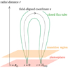 |
Fig. 1 Schematic picture of the system. One-dimensional dynamics along the axis of the closed flux tube is simulated. The axis isindicated by the dotted line, while the flux tube surface is denoted by green lines. The flux tube is intended to be nearly vertical and super-radially expanding. The geometry of the loop is defined by the filling factor f and radial distance r as functions of field-aligned distance s. |
 |
Fig. 2 Shape of the flux-tube axis defined by Eq. (7). x and z denote the horizontal and vertical coordinates, respectively. |
2.3 Basic equations
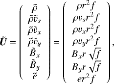
The MHD equations with the equation of state of partially ionised hydrogen, gravity, thermal conduction, radiative cooling, and phenomenology of turbulent heating are selected as the basic equations of the model, which are expressed in the form of conservation law (for derivation, see Appendix A)
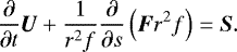 (8)
(8)
The conserved variables U and the corresponding fluxes F are given by
 (9)
(9)
where
 (10)
(10)
 (11)
(11)
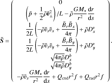
Here, eint denotes the internal energy per unit volume and is defined in Sect. 2.4. The source term S is given by
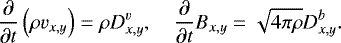
![Mathematical equation: \begin{align*} \vec{S} = \left( \begin{array}{c} 0 \\ \left(p +\dfrac{1}{2} \rho \vec{v}_{\perp}^2 \right)/L - \rho \dfrac{GM_{\odot}}{r^2} \dfrac{\textrm{d}r}{\textrm{d}s} \\ \dfrac{1}{2L} \left(- \rho v_s v_x + \dfrac{B_s B_x}{4\pi} \right) + \rho D^v_x \\ \dfrac{1}{2L} \left(- \rho v_s v_y + \dfrac{B_s B_y}{4\pi} \right) + \rho D^v_y \\ \dfrac{1}{2L} \left(v_s B_x - v_x B_s \right) + \sqrt{4 \pi \rho} D^b_x\\[1.5pt] \dfrac{1}{2L} \left(v_s B_y - v_y B_s \right) + \sqrt{4 \pi \rho} D^b_y\\ - \rho v_s \dfrac{GM_{\ast}}{r^2} \dfrac{\textrm{d}r}{\textrm{d}s} + Q_{\textrm{cnd}} + Q_{\textrm{rad}} \end{array} \right),\end{align*}](/articles/aa/full_html/2021/12/aa41563-21/aa41563-21-eq12.png) (12)
(12)
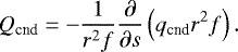
where 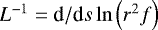 denotes the length scale of the flux-tube expansion. The conduction term Qcnd is defined in terms of conductive flux qcnd as
 (13)
(13)
Because the mean free path of an electron is generally smaller than the system size, the Spitzer–Härm flux (Spitzer & Härm 1953) is applied to qcnd:
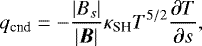 (14)
(14)
where κSH = 10−6 erg cm−1 s−1 K−7∕2. The radiative cooling Qrad and turbulent dissipation  are described in Sects. 2.5 and 2.6, respectively. Because turbulence is considered not as an external force but as a dissipative process, the losses of the kinetic and magnetic energies by turbulence are locally balanced by the gain in the internal energy. Thus, the presence of the turbulence terms does not affect the conservation of the total energy. For the same reason, we do not explicitly consider the numerical dissipation of velocity and magnetic field in the energy equation. We note that the numerical dissipation is unlikely to be the dominant heating mechanism because the coronal Alfvén wave, which has a typical wavelength of ~ 100Mm, is resolved by a sufficiently fine grid in the corona (100km).
2.4 Equation of state
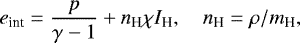
We assume that the plasma consists of neutral hydrogen atoms, protons, and electrons. The internal energy per unit volume eint is composed of the conventionalthermal energy p∕(γ − 1) and the latent heat of the ionised gas:
 (15)
(15)
where χ is the ionisation degree and nH is the number density of hydrogen atoms (proton + neutral hydrogen). IH is the ionisation energy of the hydrogen atom (IH = 13.6eV). We assume that the ionisation degree could be determined from the approximated version of the Saha-Boltzmann equation, in which only the ground state is considered as the bound state (low-temperature limit).
 (16)
(16)
where λe is the thermal de Broglie wavelength of electron.
 (17)
(17)
When chromospheric hydrogen is no longer in thermal equilibrium, the ionisation degree will deviate from the Saha–Boltzmann value (Goodman & Judge 2012), which is beyond the scope of this study. Once the ionisation degree χ is obtained, the pressure and temperature are related by
 (18)
(18)
2.5 Radiation
The radiative cooling rate per unit volume Qrad is given by
 (19)
(19)
 (20)
(20)
where p* is the pressure at the surface (photosphere) and  and
and  approximatethe optically thick and thin cooling rates, respectively. The optically thick and thin functions are seamlessly connected via ξrad. Instead of solving the radiative transfer, we model
  and
and  as follows.
The radiative heating and cooling are approximately balanced near the photosphere to maintain a nearly constant surface temperature. The optically thick radiative loss is approximated by an exponential cooling function that forces the local temperatureto approach the reference value (Gudiksen & Nordlund 2005):
 (21)
(21)
where ρ* is the photospheric mass density and  is the reference internal energy density corresponding to the reference temperature Tref. We simply assume Tref = T⊙, namely, the stellar atmosphere exhibits isothermal behaviour in the absence of other cooling/heating mechanisms.
The optically thin cooling is expressed in terms of the radiative loss function Λ(T) by ne nHΛ(T). In this work, we define the loss function over a wide range of temperature (103 K ≤ T ≤ 107 K) as follows. In the high-temperature range (T ≥ 1.5 × 10⁴ K), the cooling rate is referred from the CHIANTI atomic database with the photospheric abundance (no first ionisation potential (FIP) effect). In the low-temperature range (T ≤ 1.0 × 10⁴ K), the cooling function is deduced by Goodman & Judge (2012), which partially consider the non-LTE effect. In the intermediate-temperature range (1.0 × 10⁴ K < T < 1.5 × 10⁴ K), a bridging law between two loss functions asre employed following the method of Iijima (2016). The chromospheric heating effect by backward coronal radiation is still missing in Λ(T) defined above. To introduce this effect, we quench Λ(T) in the chromospheric temperature range, which gives 
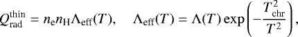 (22)
(22)
where Tchr = 2.0 × 10⁴ K. The effective radiative loss function Λeff(T) is displayed in Fig. 3, along with the original radiative loss function Λ(T) and the CHIANTI loss function defined in T ≥ 104 K.
2.6 Phenomenological model of coronal turbulence
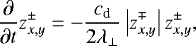
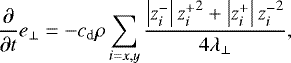
Although the mechanism of the coronal heating is debated, it is of no doubt that magnetic field feeds heat to the corona that maintains the million-Kelvin temperature by dissipation. The formation of tangential discontinuities (electric current sheets) in response to the continuous shuffling of the foot points of coronal magnetic fields is a plausible mechanism of magnetic-field dissipation (Parker 1972, 1983; Sturrock & Uchida 1981; van Ballegooijen 1986; Galsgaard & Nordlund 1996). The ubiquitous current-sheet formation should lead to small-scale impulsive energy release, which is likely to feed a sufficient amount of energy to the corona, possibly in the form of micro- and nano-flares (Parker 1988; Shimizu 1995; Aschwanden & Parnell 2002).
The formation of current sheets can be interpreted as turbulent cascading (Rappazzo et al. 2007, 2008; Verdini et al. 2012). Because the coronal loop is threaded by a strong mean magnetic field, the MHD turbulence evolving in the coronal loop can be accurately approximated by the reduced-MHD turbulence, in which the energy cascades preferentially in the perpendicular direction (Shebalin et al. 1983; Cho & Vishniac 2000; Cho & Lazarian 2003). The energy-cascading (or heating) rate of the reduced-MHD turbulence, Qheat, is precisely approximated by the mean-field quantities as follows (Hossain et al. 1995; Matthaeus et al. 1999; Dmitruk et al. 2002; Verdini & Velli 2007)
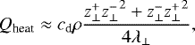 (23)
(23)
where  denotes the (root-mean-squared (RMS)) amplitude of the perpendicular Elsässer variables and λ⊥ is the correlation length of the Elsässer variable (Alfvén wave) perpendicular to the mean field. cd is a dimensionless parameter. By this approximation, we estimate the averaged heating rate using the coronal turbulence (field braiding).
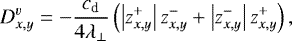
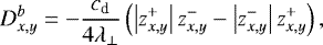
The approximated heating rate in Eq. (23) is implemented by adding the source terms  ,
,  given by Shoda et al. (2018).
 (24)
(24)
 (25)
(25)
where  . The role of these terms is explained below. Without the conservation part
  , the perpendicular components of the equation of motion and induction equation are expressed as
 (26)
(26)
In the limit of the reduced-MHD approximation (time-independent density, ∂ρ∕∂t = 0), Eqs. (24)–(26) are reduced to
 (27)
(27)
which yields the energy conservation law of
 (28)
(28)
where e⊥ is the sum of the kinetic and magnetic energies emerging from the fluctuations of the perpendicular components:
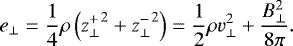 (29)
(29)
Comparing Eqs. (23) and (28), one obtain
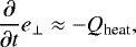 (30)
(30)
indicating that the energy dissipation by the reduced-MHD turbulence is considered appropriately.
The perpendicular correlation length is assumed to increase with the flux-tube radius, that is,
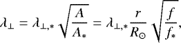 (31)
(31)
where the perpendicular correlation length at the photosphere is set equal to the typical width of the inter-granular lane: λ⊥,* = 150 km. However, the best possible free parameter cd is still debated. In this study, we infer cd = 0.1 from the previous studies of the solar-wind turbulence (van Ballegooijen & Asgari-Targhi 2017; Chandran & Perez 2019; Verdini et al. 2019).
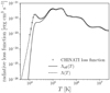 |
Fig. 3 Effective and original optically thin radiative loss functions, Λeff(T) and Λ(T), shown with solid and dashed lines, respectively. Also shown, by crosses, are the loss function from the CHIANTI atomic database with photospheric abundance. |
2.7 Boundary condition and simulation setting
Both boundaries of the simulation domain are located at the photosphere, and the photospheric temperature is fixed to the effective temperature:
 (32)
(32)
The photospheric magnetic field is known to form localised kilo-Gauss patches (Spruit & Zweibel 1979; Tsuneta et al. 2008). These patches are likely to be in thermal equipartition, which equates the gas and magnetic pressures. For the non-magnetised photosphere, the thermal equipartition field is given by
 (33)
(33)
In the magnetised photosphere, as the deeper region tends to be observed (e.g. Keller et al. 2004), the ambient gas is likely to exhibit larger pressure than the non-magnetised photosphere. Thus, the equipartition magnetic field should be larger than this equipartition value. Therefore, we set the photospheric axial magnetic field equal to
 (34)
(34)
We modelled the energy injection from the photosphere by imposing the velocity and magnetic-field fluctuations. Fluctuations were imposed at both ends of the simulation domain. The vertical and horizontal velocity fluctuations were modelled separately. The upward acoustic waves were excited on the photosphere by employing the time-dependent boundary conditions on the density and axial velocity.
 (35)
(35)
![Mathematical equation: \begin{equation*} v_{\textrm{s},\ast} = \int_{\omega^l_{\textrm{min}}}^{\omega^l_{\textrm{max}}} \textrm{d}\omega \ \tilde{v}_{\textrm{s}} \left(\omega \right) \sin \left[ \omega t + \psi^l (\omega) \right], \end{equation*}](/articles/aa/full_html/2021/12/aa41563-21/aa41563-21-eq49.png) (36)
(36)
where  is the time-averaged photospheric density,
  is the isothermal speed of sound on the photosphere, and
  is a random phase function that ranges between 0 and 2π. In the numerical implementation of the integral in Eq. (35), the frequency range was evenly divided into 21 bins and the corresponding 21 components were summed. The time-averaged photospheric density is given by equipartition on the photosphere:
 (37)
(37)
which yields
 (38)
(38)
Here,  is larger than the typical mass density on the solar surface because the magnetised photosphere should be deeper and denser. The (time-averaged) Alfvén speed vA on the photosphere is then expressed as
 (39)
(39)
We arbitrarily set  with
with
 (40)
(40)
The minimum frequency corresponds to the cut-off frequency of the acoustic wave at the photosphere (e.g. Felipe et al. 2018). The magnitude of  was tuned such that the RMS amplitude of vs,* at the photosphere is 0.6 km s−1.
 (41)
(41)
where the overline denotes the time average. Although the longitudinal-wave excitation on the photosphere is explicitly considered, the effect of the longitudinal-wave input is insignificant; the coronal temperature decreases by only 2% when the longitudinal wave injection is terminated.
The horizontal velocity and magnetic field at the bottom boundary are expressed in terms of the Elsässer variables, which are defined as
 (42)
(42)
The free boundary condition was imposed on the downward Elsässer variables.
 (43)
(43)
The upward Elsässer variable was assumed to be non-monochromatic with respect to the frequency.
![Mathematical equation: \begin{align*} z_{x,y,\ast}^+ = \int_{\omega^t_{\textrm{min}}}^{\omega^t_{\textrm{max}}} \textrm{d} \omega \ \tilde{z}^{\pm}_{x,y} \left(\omega \right) \sin \left[ \omega t + \psi^t(\omega) \right],\end{align*}](/articles/aa/full_html/2021/12/aa41563-21/aa41563-21-eq63.png) (44)
(44)
where ψt(ω) is a random phase function that ranges between 0 and 2π. As with Eq. (35), the frequency range was discretised into 21 bins when numerically implementing the integral in Eq. (44). We set  with
with
 (45)
(45)
 corresponds to the 1∕ω energy spectrum discovered in previous solar simulations and observations (Van Kooten & Cranmer 2017). Given that the typical size of a granule is 1000 km and the typical speed of surface convection is 1 km s−1 (Chitta et al. 2012), the maximum wave period corresponds to the turn-over time of granular motion. Similarly, given that the typical size of an inter-granular lane is 100 km, the minimum wave period corresponds to the turn-over time of inter-granular motion. The magnitude of
  was tuned such that the root-mean-squared amplitude of
  at the photosphere is 1.2 km s−1:
 (46)
(46)
where the overline denotes the time average. Although some solar observations have observed the suppression of convective velocity in large-filling-factor regions (e.g. Katsukawa & Tsuneta 2005), we dismiss this effect for simplicity.
By this formulation, the energy flux of the upward Alfvén wave at the footpoint of the flux tube is given by
 (47)
(47)
which is sufficiently larger than the energy flux required to sustain the solar corona (Withbroe & Noyes 1977).
2.8 Numerical method
A non-uniform grid system was used to resolve the computational domain 0 ≤ s ≤ 2lloop. A uniform cell size of Δsmin was used below the critical height s < sge, above which the cell size expands until it reaches the maximum Δsmax. In particular, in 0 ≤ s ≤ lloop, the size of the i-th cell, Δsi, was iteratively defined as
![Mathematical equation: \begin{align*} &\Delta s_i = \max \left[ \Delta s_{\textrm{min}}, \min \left[ \Delta s_{\textrm{max}}, \Delta s_{\textrm{min}} + \frac{2\varepsilon_{\textrm{ge}}}{2 + \varepsilon_{\textrm{ge}}} \left(s_{i-1} - s_{\textrm{ge}} \right) \right] \right], \nonumber \\ &s_i = s_{i-1} + \frac{1}{2} \left(\Delta s_{i-1} + \Delta s_i \right). \end{align*}](/articles/aa/full_html/2021/12/aa41563-21/aa41563-21-eq71.png) (48)
(48)
Letting N be the total number of cells, we express the cell size in the latter half of the domain lloop ≤ s ≤ 2lloop by
 (49)
(49)
The maximum cell size was fixed to Δsmax = 100 km. The relation between the minimum cell size and f* is
 (50)
(50)
This relation is used because a higher resolution is required at the transition region in the large-f* runs (for details, see Appendix B). The grid expansion rate also depends on f* as εge = 2.13 (f* < 0.05) and εge = 1.89 (f*≥ 0.05). The grid expansion height is fixed to sge = 10 000 km, which is greater than the typical height of the transition region that needs to be resolved with the minimum cell size.
In numerically solving Eq. (8), we rewrite the basic equations in terms of the cross-section-weighted conserved variables  and the corresponding fluxes
  defined by
 (51)
(51)
 (52)
(52)
where
 (53)
(53)
Using  and
and  , the basic equation is given by
 (54)
(54)
where
 (55)
(55)
With this variable conversion, any MHD solver designed for the Cartesian coordinate system can be directly applied to Eq. (54). In this study, the Harten–Lax–van Leer discontinuities (HLLD) approximated Riemann solver (Miyoshi & Kusano 2005) is used to calculate  at the cell boundary. For spatial reconstruction, the fifth-order accurate monotonicity-preserving method (Suresh & Huynh 1997) is used to reconstruct the cross-section-weighted conserved variables
  in s ≤ sge and 2lloop − s ≤ sge, whereas the monotonic upstream-centred scheme for the law of conservation (van Leer 1979) with a minmod flux limiter is used in sge < s < 2lloop − sge.
Thermal conduction and the other parts are solved independently by the second-order operator-splitting procedure as follows. First, the thermal conduction is solved for a half step Δt∕2.
 (56)
(56)
where  is the n-th step value of
  . Then, the rest of the basic equations are solved for a full step Δt.
 (57)
(57)
Finally, the thermal conduction is solved again for a half step Δt∕2.
 (58)
(58)
With this procedure, we avoid the severe constraints on the Δt from thermal conduction when updating the MHD equations.
The third-order strong-stability-preserving (SSP) Runge–Kutta method is used in the time integration of the MHD equations (Shu & Osher 1988; Gottlieb et al. 2001). The super-time-stepping method (Meyer et al. 2012, 2014) is used to solve the thermal conduction, which reduce the numerical cost and time with minimum loss of accuracy.
3 Simulation result
3.1 Fiducial (solar) case: atmosphere and spectrum
First, we discuss the simulation run with lloop = 20 Mm and f* = 1.0 × 10⁻² as the fiducial case. In this case, the coronal field strength is ≈20 G, which is within the range of the solar coronal magnetic field strength measured by the coronal seismology technique (Nakariakov & Ofman 2001; Verwichte et al. 2004; Jess et al. 2016), and thus the fiducial case is regarded as the solar case.
Figure 4 illustrates the time-averaged properties of a quasi-steady coronal loop. Panels show the mass density (top) and temperature (middle) along the loop axis and the differential emission measure (DEM, bottom), defined by
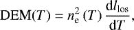 (59)
(59)
where ne(T) is the electron density withtemperature T and llos is the lengthalong the line of sight. Practically, dividing the temperature range into bins and considering the vertical line of sight (llos = r), the DEM and associated emission measure distribution (EMD) are numerically obtained as follows
 (60)
(60)
where ne(Ti) is the total number density of an electron that exhibits a temperature in [Ti − ΔTi∕2, Ti + ΔTi∕2] and Δr(Ti) is the total radial extension of where Ti − ΔTi∕2 ≤ T < Ti + ΔTi∕2. The DEM is calculated in the temperature range of 104 K ≤ T ≤ 107 K with an equal spacing in the logarithmic scale of T. The DEM in the range of T < 104 K is not calculated because, in the low-temperature range, the atmosphere is not optically thin and the DEM loses its meaning. We note that the unit of EMD is cm−5, while the ‘volume’ EMD, which has often been used in the literature (Güdel et al. 2003; Scelsi et al. 2005), represents the distribution of an emission measure over the whole coronal volume and has a different unit (cm−3).
The high-temperature (T > 106 K) corona is successfully reproduced in the fiducial case. Since we are imposing the phenomenological, mean-field formulation of the coronal heating (field braiding/turbulence), the heating tends to be more constant in time and more uniform in space than the actual three-dimensional case in which the heating is intermittent in time and space. Nevertheless, the time-averaged heating rateshould be similar between the 1D approximation and the 3D simulation, because the previous 3D simulation of solar wind yielded a similar mean field to the 1D simulation with turbulence phenomenology (Shoda et al. 2019).
Under the assumption that the upper atmosphere (T ≥ 104 K) is optically thin in the wavelength of interest, the XUV spectrum is obtained from the EMD using the open-source package ChiantiPy based on CHIANTI database ver 10.0 (Del Zanna et al. 2021). In particular, the specific intensity Iλ was calculated from the EMD using the ChiantiPy.core.Spectrum module with the coronal abundance given by Schmelz et al. (2012). Although the radiative loss functionΛ(T) is constructed with photospheric abundance, because the loss function is nearly independent of the FIP effect in the radiation-dominated temperaturerange T ≤ 3 × 10⁵ K, the inconsistency in abundance do not violate the simulation results. Assuming that the stellar corona is a uniformly bright sphere, the spectral flux density at the heliocentric distance r is deduced by (see, for example, Sect. 1.3 of Rybicki & Lightman 1979)
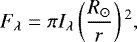 (61)
(61)
which yieldsthe X-ray and EUV luminosities as
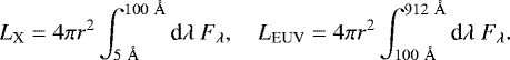 (62)
(62)
In terms of energy, X-ray photons are in the range of 0.12−2.48 keV. Caution must be exercised when calibrating the X-rays because a subtle difference in the bandpass of the instrument can result in large differences in the derived response function and X-ray luminosity (Zhuleku et al. 2020). The procedure for the translation between different instruments is available in Judge et al. (2003).
To test the capability of our model in the prediction of XUV spectrum, we compare in Fig. 5 the spectral flux density obtained from our simulation (red) and that from the observation in a solar activity minimum (blue). The observed spectrum is obtained from the coordinated observation in the Whole Heliosphere Interval (WHI, from March 20, 2008, to April 16, 2008, Woods et al. 2009; Chamberlin et al. 2009). Figure 5 shows that, below the Lyman edge (≤ 912 Å), the simulated spectrum is in a good agreement with the observed spectrum. Above the Lyman edge (≥ 912 Å), the continuum is underestimated, and the emission lines are overestimated in the simulated spectrum, possibly because the optically thin approximation is inadequate in this wavelength range. In this study, because the focus is on the spectrum below the Lyman edge, the simulation is validated with respect to spectrum prediction.
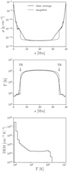 |
Fig. 4 Simulated loop properties of the fiducial case. Top: time-averaged (solid line) and snapshot (dashed line) profiles of mass density along the loop axis. Middle: time-averaged (solid line) and snapshot (dashed line) profiles of temperature along the loop axis. Bottom: time-averaged differential emission measure (solid line). Annotations ‘TR’ in the middle panel indicate the locations of the transition region in the snapshot profile. |
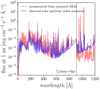 |
Fig. 5 Observed (blue) and simulated (red) spectral flux density of the Sun measured at 1 au. The observed spectrum is retrieved in the solar activity minimum. The two spectra are in a good agreement below the Lyman edge (≤912 Å). |
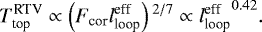
3.2 Loop-length dependence: density and temperature
The coronal loop length is a fundamental parameter that affects the coronal density and temperature. Here, we show the relation between the time-averaged coronal properties and the coronal loop length. For simplicity, we fix the magnetic filling factor to the fiducial (solar) value: f* = f⊙ = 0.01. Hereinafter, the time-averaged value of X will be denoted by Xave.
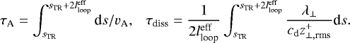
In the discussion on the behaviour of the coronal properties, the results must be compared with the analytical RTV scaling law (Rosner et al. 1978). We note that the half-loop length in the RTV scaling law denotes the length from the transition region to the apex of the loop, whereas lloop stands for the length from the stellar surface to the apex of the loop. For better comparison, instead of lloop, we use the effective half-loop length  , which denotes the coronal length, and is defined as
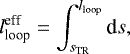 (63)
(63)
where sTR (< lloop) is where Tave = 105 K.
Another factor that should be considered is the gravitational stratification. The effective half-loop length often exceeds the coronal pressure scale height. In such cases, the loop-top pressure in the original RTV scaling law is replaced by the coronal-base pressure (Serio et al. 1981). Given that the pressure is continuous across the transition region, we define the coronal-base pressure pbase as the pressure measured at Tave = 105 K. For the coronal electron density, both the loop-top value ne,top and coronal-base value ne,base are measured. In contrast to pressure, the density is discontinuous across the transition region, and therefore the definition of the coronal-base density is not trivial. Here, we define ne,base as the value measured in the coronal base:
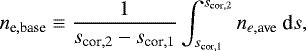 (64)
(64)
where we set scor,1 = 10 Mm and scor,2 = 15 Mm. The loop-top density and temperature are given by
 (65)
(65)
Figure 6 shows the  dependencesof the time-averaged coronal properties (density, temperature and pressure). The loop-top temperature and coronal-basepressure obey a power–law relation with respect to the effective half-loop length, which is formulated as
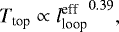 (66)
(66)
 (67)
(67)
The (generalised) RTV scaling law predicts that the loop-top temperature obeys the following relation
 (68)
(68)
where we dismiss the exponential correction term as it is negligible (Serio et al. 1981). A comparison of Eqs. (66)–(68) reveals that the simulation results are consistent with the RTV scaling law.
An alternative form of the RTV scaling law predicts a relation among the coronal energy flux Fcor, loop length  , and loop-top temperature
 , and is expressed as
 (69)
(69)
A comparison of Eqs. (66) and (69) indicates that the energy flux injected into the corona is larger for longer loops. In terms of the heating rate per unit volume Q, the RTV predictions,
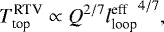 (70)
(70)
 (71)
(71)
and simulation results from Eqs. (66) and (67) indicate that 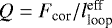 is a decreasing function of
  . These conclusions shall be directly validated in the following section.
The bottom panel of Fig. 6 shows the variations in loop-top and coronal-base electron densities over  . Given that the RTV scaling law predicts a larger loop-top density at a higher loop-top temperature for a uniform corona, the decrease in the loop-topdensity is attributed to gravitational stratification. We note that the coronal-base density exhibits a weaker dependence on
  than the coronal-base pressure, which is contradictory if the coronal-base temperature is constant in
  . It may be interpreted that the coronal-base temperature increases with
  in response to the increasing Ttop with
  .
.
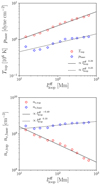 |
Fig. 6 Coronal-property dependences on the effective loop length. Top: relation between the effective half loop length
|


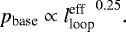
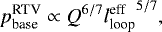
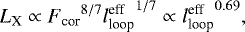
3.3 Loop-length dependence: energy flux and XUV emission
For a better interpretation of the behaviour of coronal properties, the variation in the energy flux entering the corona Fcor with the effective half-loop length  must be revealed.
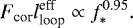
Directly measuring Fcor from the simulation data is, however, not a trivial task. To obtain Fcor, one needs to measure the energy flux at the base of the corona, which moves in time and is broadened after time averaging. Because a significant amount of energy is reflected back at the transition region, a slight difference in the position of the coronal base yields a significant error or uncertainty in Fcor. Therefore, instead of directly measuring Fcor, we measure the backward conductive flux Fcnd, which should be balanced with Fcor by energy conservation.
The top and bottom panels in Fig. 7 show the loop-length (lloop and  ) dependence of the coronal conductive flux. The panels display the simulation runs with a fixed magnetic filling factor of f* = 1.00 × 10⁻². The red circles and blue diamonds represent the conductive flux measured at Tave = 1.0 × 10⁶ K and averaged over 10 Mm ≤ s ≤ 15 Mm, respectively.The black solid lines represent the power-law fittings to the blue diamonds. The coronal conductive flux increases with the loop length. However, the trend deviates from a simple power law. When the loop length is sufficiently small (
 ) or large (
 ), the conductive flux weakly depends on the loop length. The energy flux increases around
  , with the minimum and maximum values differing by a factor of four.
An approximate power-law fit to the blue diamonds yields the following scaling law
 (72)
(72)
which, in combination with the RTV scaling law, predicts
 (73)
(73)
The simulated dependence of Ttop on  , Eq. (66), is reproduced by the semi-analytical arguments. Thus, the results shall be explained semi-analytically once the theoretical behaviour ofFcor (or equivalently Fcnd) has been derived. In Sect. 4, we propose a simple model to produce Fcor.
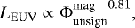
The enhanced energy injection to the corona produces enhanced XUV emissions. Figure 8 depicts the loop-length dependence of the predicted XUV luminosity. For each coronal loop calculation, the XUV spectrum is calculated as in Fig. 5 and converted to XUV luminosity through Eq. (62). Both LX and LEUV exhibit increasing trends as those found in the coronal energy flux Fcnd. In particular, LX exhibits thistrend significantly. The inferred power–law relations are
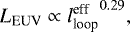 (74)
(74)
 (75)
(75)
The dependence of LX on  is further explained semi-analytically. The X-ray luminosity should be proportional to the emission measure of the corona, that is,
 (76)
(76)
where ncor is the typical number density of the coronal loop that lies between nbase and ntop. Assuming that ncor follows the prediction of the RTV scaling law,
 (77)
(77)
the X-ray luminosity is connected to the coronal energy flux Fcor and loop length  by
by
 (78)
(78)
where the simulated scaling law Eq. (72) is used in the second proportional relation. The actual scaling relation Eq. (75) is in good agreement with the semi-analytical prediction Eq. (78), validating the RTV scaling law in describing the stellar coronal properties.
We note that EUV luminosity LEUV is weakly dependent on the loop length compared with LX because a portion of the EUV photons originates from the upper chromosphere and transition region, which are barely affected by the variation in the coronal loop length. Within the investigated loop-length range, the ratio LEUV∕LX decreases from ~10 to ~ 3 as the effective loop length increases.
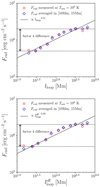 |
Fig. 7 Relation between the coronal conductive flux and loop length. Top: half loop length versus coronal conductive flux measured at Tave = 106 K (red circles) and averaged in 10 Mm ≤ s ≤ 15 Mm (blue diamonds). Also shown, by the solid line, is the power-law fitting to the blue diamonds. Bottom: same as the top panel but with respect to the effective half loop length
|

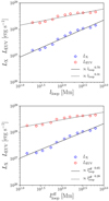 |
Fig. 8 (Effective) loop length versus X-ray luminosity LX (red circles) and EUV luminosity LEUV (blue diamonds). The solid and dashed lines show the power-law fittings to the simulation results. The top and bottom panels show the relation with respect to the half loop length lloop and the effective hal loop length |

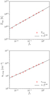 |
Fig. 9 Magnetic filling factor on the photosphere f* versus time-averaged loop-top temperature (Ttop, top panel) and loop-top electron density (ne,top, bottom panel). The half loop length is fixed to lloop = 20 Mm. Red circles show the simulation results and the solid lines show the power-law fittings to them. |
3.4 Filling-factor dependence: density and temperature
The magnetic filling factor of the photosphere appears to have scaled with the Rossby number, or equivalently the magnetic activity level (Saar 1996, 2001; Reiners et al. 2009). Hence, the dependence of the coronal properties on the filling factoris worth investigating as a proxy of the dependence of the stellar corona on the activity level. The simulation results with various magnetic filling factors shall be discussed below, with the half-loop length fixed to lloop = 20 Mm.
Figure 9 shows the filling-factor dependence of the time-averaged loop-top temperature Ttop and electron density ne,top. The coronal density and temperature increase with an increase in the magnetic filling factor following a power–law relationship
 (79)
(79)
 (80)
(80)
Although not explicitly demonstrated, the effective half-loop length also weakly depends on f* as
 (81)
(81)
We note that the RTV scaling law semi-analytically predicts a relation of
 (82)
(82)
which is close to the simulation result Eq. (79). Alternatively, in terms of the heating rate per unit volume Q, the RTV scaling law coupled with Eqs. (79) and (81) yields
 (83)
(83)
while the RTV scaling law Eqs. (80) and (81) yield
 (84)
(84)
The two trends are mostly consistent with each other.
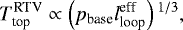
The RTV scaling law predicts that the loop-top temperature Ttop depends on the coronal energy flux Fcor and effective half-loop length  as Eq. (69). A comparison between Eqs. (69) and (79) reveals the mostly proportional relationship between Fcor and f*:
 (85)
(85)
which shall be further investigated in the following section.
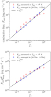 |
Fig. 10 Relation between filling factor and coronal conductive flux. Top: magnetic filling factor on the photosphere f* versus backward conductive flux measured in the corona. The half loop length is fixed to lloop =20 Mm. The red circles and blue diamonds represent the flux measured at Tave = 106 K and averaged in 10 Mm ≤ s ≤ 15 Mm. The black solid line is the power-law fitting to the blue diamonds. Bottom: same as the top panel but the vertical axis denotes |

3.5 Filling-factor dependence: energy flux and XUV emission
The energetics of the corona with various magnetic filling factors shall be discussed here. The top panel of Fig. 10 shows the relation between the filling factor f* and the coronal backward conductive flux measured at Tave = 106 K (red circles) and averaged over 10 Mm ≤ s ≤ 15 Mm (blue diamonds). The two conductive fluxes exhibit different behaviours, with the red circles appearing to saturate within the large f* limit. This difference may arise from the different physical meanings of Tave = 106 K, where the values of the red circles are measured. Tave = 106 K is located near the loop top for the small f* cases and near the transition region for the large ones. Therefore, the blue diamonds may be interpreted as the coronal energy flux.
Given the dependence of the loop-top temperature and RTV scaling law on the filling factor, the relation among the coronal energy flux Fcor, effective loop length  , and filling factor f* is predicted by Eq. (85). This prediction is confirmed in the bottom panel of Fig. 10, which shows the following scaling relation:
 (86)
(86)
This consistency indicates that the RTV scaling law must be applicable to stellar coronae with varying activity levels. The simulation results validate the previous studies on stellar coronal energetics based on the RTV scaling law (Shibata & Yokoyama 2002; Takasao et al. 2020).
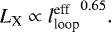
Figure 11 shows the spectra of XUV emission for different magnetic filling factors. For all wavelengths below the Lyman edge (912 Å), the XUV emissions increase as the magnetic filling factor increases. This is a natural consequence of the increased coronal density shown in Fig. 9. In particular, as seen in the central panels of Fig. 11, the enhancement of the energy flux from f* = 0.01 to f* = 1 is centred on ~ 10 with a variance of factor ~5 in the EUV range (100 Å < λ ≤ 912 Å), whereas a significantly larger enhancement occurs in the X-ray range (5 Å < λ ≤ 100 Å). This is because of the sensitivity of the X-ray emissivity to the temperature. Also shown in the right panels of Fig. 11 are the spectra of the total photon number emitted from the star per unit time (photon number luminosity) given by 4πr2λFλ∕(hc). For all f*, the spectrum of the photon number luminosity is flatter than the energy spectrum, implying that the photon population with respect to wavelength is approximately uniform in the XUV range.
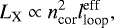
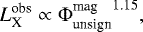
The magnetic-flux dependences of the X-ray luminosity LX and EUV luminosity LEUV are also investigated. Figure 12 reveals the variation in LX (blue diamonds) and LEUV (red circles) with the unsigned magnetic flux  defined by
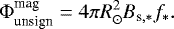 (87)
(87)
Because the photospheric magnetic field is fixed, the filling factor f* is the only variable in the definition of  . We find thatboth LX and LEUV follow power laws with respect to
  and are expressed as follows
 (88)
(88)
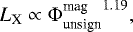 (89)
(89)
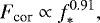
which are represented by the solid and dashed lines in Fig. 12, respectively. A scaling law is observationally discovered between the unsigned magnetic flux and the X-ray luminosity (Pevtsov et al. 2003)
 (90)
(90)
which is shown by the dotted line in Fig. 12. Although the magnitudes of the X-ray luminosity from the simulation are smaller than the observed values, possibly because the proposed model reproduces the coronal properties in the activity minimum (a quiet, quasi-steady corona without flaring activities), the power-law index from the simulation (1.19) is nearly identical to that from the observation (1.15). The reproduction of the observational  –LX relation provides another support to our model. The proposed
  –LEUV relationship, Eq. (88), can be tested by the Sun-as-a-star observations in the EUV range (e.g. Toriumi et al. 2020).
The filling-factor dependence of the EUV photon number luminosity  is also investigated.
  is defined as the total number of EUV photons emitted from the star, that is,
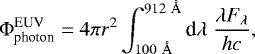 (91)
(91)
which acts as a proxy of the photo-ionised hydrogen number per unit time. Figure 13 shows the EUV photon number luminosity with varying magnetic filling factors. As with LEUV,  also follows a power law with respect to f*, which is given by
 (92)
(92)
A comparison of Eqs. (88) and (92), reveals that LEUV and  follow marginally different power laws with respect to f* (or equivalently
  ).
).
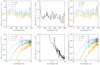 |
Fig. 11 Filling-factor dependence of the XUV spectrum. Left: spectral energy flux at 1 au for f* = 0.01 (orange, solid), f* = 0.1 (green, dashed), and f* = 1 (blue, dotted). Centre: energy-flux ratio of f* = 1 to f* =0.01. Right: photon-number luminosity spectrum for f* = 0.01 (orange, solid), f* = 0.1 (green, dashed), and f* = 1 (blue, dotted). Bottom panels are the same as top panels but with logarithmic x axis thatemphasise the short-wavelength region. For better visualisation, spectra are averaged over 20 Å-bins in the top panels. |
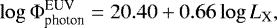
3.6 LX –LEUV and LX – relations
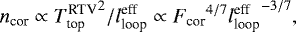
One of the objectives of this study is to propose a method to estimate the stellar EUV luminosity LEUV from other observable quantities. Because the X-ray luminosity LX is measurable and should be correlated with LEUV (see e.g. Sanz-Forcada et al. 2011), the relationship between LX and LEUV over a wide range of filling factors and loop lengths warrants investigation.
The top panel of Fig. 14 highlights the correlation between X-ray luminosity LX and EUV luminosity LEUV. The black circles correspond to the simulation runs listed in Table 2. Although the simulation runs are spread over wide ranges in the filling factor and loop length, a single power-law fit adequately applies to the LX –LEUV relation, which is given by
 (93)
(93)
where LEUV and LX are measured in the unit of erg s−1. The red points with the vertical error bars indicate the observational estimation by Sanz-Forcada et al. (2011). The pure theoretical estimation of LEUV in this study conforms with the pure observational estimation of the same by Sanz-Forcada et al. (2011). Although the power-law index of LX –LEUV relation is 0.86, according to Sanz-Forcada et al. (2011), the coefficient 0.67 in Eq. (93) is, in fact, close to the observational value (0.681) derived from the Extreme Ultraviolet Explorer (EUVE) observations (Johnstone et al. 2021). The fact that the independent methods produces a similar LX –LEUV relation validates the proposed model of stellar coronae and their XUV emissions.
The correlation between the X-ray luminosity LX and the EUV photon-number luminosity  is also highlighted in the bottom panel of Fig. 14. They, too, follow a power–law relationship given by
 (94)
(94)
where  is measured in unit of s−1.
Simulation runs conducted in this study.
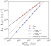 |
Fig. 12 Unsigned magnetic flux |

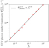 |
Fig. 13 Magnetic filling factor on the photosphere f* versus photon number luminosity in the EUV range. Each simulation run corresponds to each red circle. The black solid line shows the power-law fitting to the simulation results. |
4 Analytical arguments on coronal energy flux
Several scaling relations with respect to the loop length and magnetic filling factor are provided in Sect. 3. In this section, we analytically describe the coronal energy injection process governing the scaling relations. Because energy is mainly transported as transverse fluctuations of the velocity and magnetic field (Alfvén waves), the efficiency of Alfvén-wave transmission into the corona is key to the analysis. This section is devoted to reviewing the linear theory of Alfvén-wave propagation in a stellar atmosphere and to provide analytical arguments for the origin of the scaling laws discovered through the simulation.
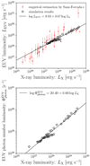 |
Fig. 14 Inferred relations between X-ray luminosity and EUV emission. Top: correlation between the X-ray luminosity LX and EUV luminosity LEUV. X-ray and EUV are defined in terms of wavelength λ as 5 Å < λ ≤ 100 Å and 100 Å < λ ≤ 912 Å, respectively. Each black circle corresponds to the simulation run listed in Table 2, and the black solid line shows the power-law fitting to them. Also shown, by the red points with vertical error bars, are the empirical estimation by Sanz-Forcada et al. (2011). Bottom: same as the top panel but for the X-ray luminosity
LX and photon number luminosity |

4.1 Linear theory of Alfvén-wave propagation and reflection
A significant amount of Alfvén waves excited at the photosphere is reflected before reaching the solar corona (Cranmer & van Ballegooijen 2005; Verdini & Velli 2007). The relationship between the Alfvén-wave transmission efficiency and the loop properties in the linear regime remains unclear and shall be discussed in this section.
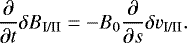
Figure 15 illustrates the schematic of the concerned system. The convection–magnetic field interaction excites the Alfvén waves propagating upwards along the expanding flux tube. In our simulation setting, the Alfvén speed is maintained at a nearly constant value during the tube expansion (Eq. (4)). Because the Alfvén-wave reflection is triggered by a gradient in the Alfvén speed (Stein 1971; An et al. 1989; Vasquez 1990), the Alfvén waves reflected in the flux-tube expansion region are feeble. Therefore, the bulk of the reflection occurs in a layer between the flux-tube merging height (where the flux-tube expansion ends) and the coronal base, which is in between the two vertical dashed lines in Fig. 15.
The Alfvén waves travelling through the reflection layer is considered in the following analysis. For simplicity, the thickness of the layer is disregarded. This approximation is validated by the fact that the reflection-layer thickness (~ 100 Mm) is notably smaller than the typical wavelength of Alfvén waves therein (~ 101−2 Mm). Then, the problem is simplified as a linear-wave transmission through a discontinuity, as described in the lower part of Fig. 15. Hereinafter, we denote the variables in the region on the left/right of the discontinuity as region I/II, respectively.
The equation describing the Alfvén-wave propagation is
![Mathematical equation: \begin{align*} \left[ \frac{\partial^2}{\partial t^2} - v_{A,\textrm{I/II}}^2 \frac{\partial^2}{\partial s^2} \right] \delta v_{\textrm{I/II}} = 0, \end{align*}](/articles/aa/full_html/2021/12/aa41563-21/aa41563-21-eq160.png) (95)
(95)
the solution of which is given by
 (96)
(96)
We note that aI/II (bI/II) denotes the amplitudes of the upward (downward) propagating Alfvén wave in region I/II, respectively. Given the frequency ω, the dispersion relation yields the wavenumber kI/II in each region.
 (97)
(97)
The corresponding magnetic-field fluctuation is deduced from the linearised induction equation, that is,
 (98)
(98)
Because the fluctuations of the velocity and magnetic field are required to be continuous across the boundary, the amplitudes must satisfythe following relations.
 (99)
(99)
 (100)
(100)
Solving these two equations yields
 (101)
(101)
The energy transmission rate TAW is defined asthe ratio of the forward-propagating Alfvén-wave energy in regions I and II. Namely,
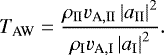 (102)
(102)
We obtain a general form of the energy transmission rate within the limit of ρII ∕ρI ≪ 1 by combining Eqs. (101) and (102):
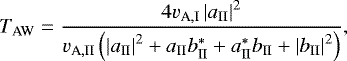 (103)
(103)
where X* denotes the complex conjugate of X. It is interesting to see that the energy transmission rate depends on the values of aII and bII, namely, the wave population in region II (corona).
The transmission rate in the two limiting cases are investigated below. When bII = 0 (no Alfvén waves propagating towards the chromosphere), the energy transmission rate is given by (Hollweg 1984)
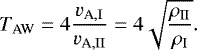 (104)
(104)
The other limiting case is bII = aII (forward and reflected Alfvén waves are equally abundant in the corona), where the transmission rate is given by
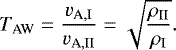 (105)
(105)
To summarise, the transmission rate of Alfvén wave is given by
 (106)
(106)
where the value of cref depends on the population ratio of the forward and backward Alfvén waves in region II.
In the numerical model implemented in this study, the density in the region I should be the mass density at the flux-tube merging height s = hmerge. In the flux-tube model employed in this model, hmerge is expressed as
 (107)
(107)
where H* is the density scale height at the photosphere (see Eq. (5) for definition). Assuming that the density scale height is uniform in 0 ≤ s ≤ hmerge, we can write the mass density at the merging height ρmerge as
 (108)
(108)
Then, using Eq. (102), we obtain the Alfvén-wave transmission rate for our model as
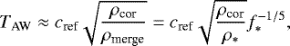 (109)
(109)
where ρcor denotes the mass density at the coronal base. We note that a large f* could lead to a small transmission rate, when ρcor does not increase faster than  .
.
 |
Fig. 15 Model of Alfvén-wave transmission across a free boundary with density jump. |
4.2 Loop-length dependence of the coronal energy flux
In Sect. 3.3, it is shown that the coronal energy flux increases with lloop but saturates at approximately four times the value of the short-loop limit (see Fig. 7). This behaviour is naturally explained by the theory of Alfvén-wave transmission.
The bottom panel of Fig. 6 shows that the mass density of the coronal base remains mostly constant with respect to the loop length. Then, according to Eq. (109), the change in the coronal energy flux is attributed to the change in the value of cref. Because 1 ≤ cref ≤ 4, the coronal energy flux should saturate at approximately four times the basal value, as observed in Fig. 7.
The enhancement of the coronal energy flux at  can be explained in terms of the timescales of Alfvén-wave propagation and dissipation. The backward waves in the corona are originated from the other base of the corona. The backward waves are subject to the turbulent dissipation during their propagation, which results in a smaller amplitude at the reflection layer than the amplitude of the forward waves. The population ratio,
  , should thus depends on the ratio of the Alfvén-crossing time τA to the turbulent dissipation time τdiss, which are respectively defined as
 (110)
(110)
When τA∕τdiss < 1, the coronal Alfvén waves propagating from one coronal base to the other hardly experience any turbulent dissipation. Therefore, the population ratio  should tend to unity in this case. When τA∕τdiss > 1, the coronal Alfvén waves significantly dissipate during the propagation through the corona. Thus, the population ratio
  should be far from unity in this case.
This argument is substantiated by Fig. 16, in which τA (red circles) and τdiss (blue diamonds) are plotted against the half-loop length lloop. The Alfvén crossing time is shorter than the turbulent dissipation time in lloop < 102 Mm and vice versa in lloop > 102 Mm. Therefore, it is likely that, when lloop < 102 Mm, the weak turbulent dissipation yields 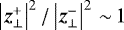 and cref ≈ 1. In the opposite limiting case of lloop > 102 Mm, the backward Alfvén waves significantly decay in the coronal loop, resulting in
 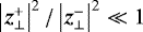 and cref ≈ 4. These arguments underscore the importance of the timescale of turbulent dissipation in a coronal loop.
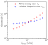 |
Fig. 16 Half loop length versus timescale of Alfvén-wave crossing (τA red circles) and Alfvén-wave turbulent dissipation (τdiss, blue diamonds). For the definitions of τA and τdiss, see Eq. (110). |
4.3 Filling-factor dependence of the coronal energy flux
In Sect. 3.5, the coronal energy flux is found to follow a power law as a function of f* :
 (111)
(111)
or alternatively
 (112)
(112)
These power-law relations are explained by the combined effect of the RTV scaling law and the energy transmission rate Eq. (109). In the absence of the Alfvén-wave dissipation in the chromosphere, the energy flux injected into the corona is given by
 (113)
(113)
where FA,* is the upward Alfvén-wave energy flux at the footpoint of the flux tube, which is fixed for all the simulation runs. According to the RTV scalinglaw, the density and the coronal energy flux are related by
 (114)
(114)
Eqs. (113) and (114) yield
 (115)
(115)
where we use  . As addressed in the previous section, the value of cref depends on the balance between the Alfvén-crossing timescale τA and the turbulent dissipation timescale τdiss in the coronal loop. Given that a larger f* yields a smaller τA∕τdiff (as well as a smaller cref), the predicted dependence of cref on f* is
 (116)
(116)
where αref > 0. Given the limited range of cref (1 ≤ cref ≤ 4), the power index αref is small. Then, the semi-analytical scaling relation,
 (117)
(117)
conforms with the obtained scaling relation Eq. (112).
 |
Fig. 17 Rossby number versus normalised X-ray luminosity (blue diamonds). The Rossby number and the filling factor are connected by Eq. (118). Results for the fixed half loop length lloop =20 Mm are shown. Also shown, by the solid and dashed lines, are the observational relation by Pizzolato et al. (2003) and its scaled-down version (1/8). |
5 Discussion
5.1 Inferred Ro–LX relation
The X-ray behaviour with respect to the stellar Rossby number has been established in the literature (Pizzolato et al. 2003; Wright et al. 2011, 2018; Wright & Drake 2016; Magaudda et al. 2020). By prescribing a relation between the filling factor f* and the Rossby number Ro, we compare the model prediction with the observational relation. The magnetic filling factor follows a power-law relation with respect to the Rossby number (Saar 1996, 2001; Reiners et al. 2009). Given that the magnetic activity saturates at Ro ∕Ro⊙≈ 0.1 and f⊙ ≈ 0.01, the power–law relationship is assumed as follows.
![Mathematical equation: \begin{align*} f_{\ast} = \min \left[1, \ f_{\odot} \left(\frac{\textrm{Ro}}{\textrm{Ro}_{\odot}} \right){}^{-2} \right].\end{align*}](/articles/aa/full_html/2021/12/aa41563-21/aa41563-21-eq191.png) (118)
(118)
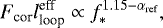
Figure 17 shows the relation between Ro∕Ro⊙ given by Eq. (118) and LX∕L⊙. The blue diamonds represent the simulation results, and the black solid line represents the observational relation observed in Sun-like stars (Pizzolato et al. 2003). Although a gap exists between the simulation results and the observational relation, when the observational relation is scaled down by a factor of eight (represented by the dashed line), the simulation results conform with the observations. Given that the observational data points have a large scatter (an order of magnitude in LX ∕L⊙), and that the proposed model corresponds to the activity minimum where the X-ray luminosity is 10–20 times smaller than the activity maximum (Johnstone & Güdel 2015), the simulation results adequately corroborate with the observations.
5.2 Missing physics and limitations
Although our model self-consistently solves the physical processes of energy injection into the corona, turbulent coronal heating, and thermal responses of the coronal loop, several other physical processes have not been considered as listed below.
The impulsive nature of the coronal heating is disregarded. The phenomenological turbulent dissipation implemented in this study yields the time-averaged heating rate, whereas the actual coronal heating is highly intermittent in space and time, as indicated by previous simulation studies (Einaudi et al. 1996; Cassak et al. 2008; Dahlburg et al. 2016; Kanella & Gudiksen 2018) and observations (Cirtain et al. 2013; Testa et al. 2014; Ishikawa et al. 2017; Antolin et al. 2021). In the presence of localised heating, the DEM extends to the high-temperature side, possibly forming the bi-modal structure observed in active stellar coronae (Güdel et al. 1997). The accuracy of the DEM obtained in this 1D simulation must be tested in the future.
The coronal loop is assumed to be isolated from the ambient plasma. However, previous studies have stated that the interface between the coronal flux tube and its surrounding is a preferential region for heating by phase mixing and resonant absorption (Ionson 1978; Heyvaerts & Priest 1983; Hollweg & Yang 1988; Sakurai et al. 1991; Hood et al. 2002; Pagano & De Moortel 2019; Van Damme et al. 2020). In fact, resonant absorption is observed to occur in the solar corona (Antolin et al. 2015; Okamoto et al. 2015). Although there is no scientific consensus on the ability of phase mixing and/or resonant absorption to feed sufficient thermal energy to the corona, the relation between these processes and XUV emissions must be investigated.
Energy injection by the emergence of magnetic field from the stellar interior (magnetic flux emergence, Takasao et al. 2013) was dismissed. Recent observations of the solar corona indicate that the coronal loops are preferentially heated near the bottom (Berghmans et al. 2021), possibly by its interaction (magnetic reconnection) with adjacent small-scale loops (Chen et al. 2021). Because the (small-scale) coronal loops are formed by the magnetic flux emergence, these observations imply that a fraction of the coronal energy must be supplied by the emergence. Indeed, a recent work on the solar wind indicates the considerable role of magnetic flux emergence in the injection of energy to the open-field regions (Wang 2020).
Throughout this study, the energy spectrum is reconstructed from EMD (DEM) under the optically thin approximation. Although this approximation has been widely used (Sanz-Forcada et al. 2011; Duvvuri et al. 2021), it must be tested in future under a realistic treatment of radiative transfer. For example, the Lyman continuum appears to be optically thick, with an extended source region in the upper chromosphere (Avrett & Loeser 2008). Other studies have claimed that a simple optically thin treatment of the coronal lines may produce incorrect results (Schrijver et al. 1994). To solve this issue, the frequency-dependent radiative transfer equation must be solved in the future.
In converting the single-loop properties retrieved from the simulation results to a global quantity such as LX, we assume thatthe stellar corona has a uniform brightness. The brightness of the actual stellar coronae, however, may be highly structured, as seen in the solar corona. Because emissions from a single active region depends on its size, the size distribution of active regions over the entire stellar surface affects the measured distribution of the total coronal emissions from the star (Takasao et al. 2020). The effect of coronal structuring must be considered in the future by, for instance, the global modelling ofstellar coronae (van der Holst et al. 2014; Alvarado-Gómez et al. 2016; Oran et al. 2017; Airapetian et al. 2021).
These issues need to be considered in future model improvements.
5.3 Extension to other types of stars
In this study, we focused on the main-sequence Sun-like stars that exhibit solar mass, solar radius, solar luminosity, and solar metallicity. Therefore, the application of Eqs. (93) or (94) to other classes of stars would require additional considerations.
First, M-type stars are of particular interest in the context of exoplanet because they occupy a large fraction of the local stellar population (Bochanski et al. 2010; Winters et al. 2019) and often host terrestrial planets within the habitable zones (Bonfils et al. 2013; Dressing & Charbonneau 2015). The applicability of the proposed theoretical predictions to lower-mass stars (especially, M dwarfs) must be investigated in the future. Given the lower metallicity of old M-type stars, the dependence of XUV emissions on metallicity must also be studied (Washinoue & Suzuki 2019). According to Fig. 14 in Johnstone et al. (2021), a single power law between LX and LEUV could be found in low-mass stars with various spectral types, and thus Eqs. (93) and (94) may be directly applicable to lower-mass stars.
Second, the XUV emissions of pre-main-sequence stars significantly alter the evolution of proto-planetary discs and planet formation (Gorti & Hollenbach 2009; Nakatani et al. 2018; Wang et al. 2019). In the case of pre-main-sequence star accretion (classical T-Tauri stars), two effects of accretion on XUV emissions must be considered. First, the XUV emissions from the accretion shocks could be comparable to or even greater than those from the corona (Günther et al. 2007). Second, because the accretion to the stellar surface may excite velocity disturbances on the photosphere, the Alfvén-wave energy injected into the corona is likely to be enhanced (Cranmer 2008, 2009). A model that considers these accretion effects is required to theoretically predict the XUV emissions from pre-main-sequence stars.
6 Conclusion
In this study, we theoretically investigate the coronal properties of the Sun and Sun-like stars. The simulation domain extends from the solar surface to the corona, with energy transport from the surface and dissipation in the corona being solved in a self-consistent manner. The thermal structuring of the stellar atmosphere is also reproduced by implementing thermal conduction and radiative cooling. The behaviours of the coronal properties with respect to the loop length and magnetic filling factor are explained by a combination of the behaviour of the coronal energy flux and the RTV scaling law. With the parameter survey, we reproduce the nearly linear relation between the unsigned magnetic flux and the X-ray luminosity. Scaling relations between the EUV properties (luminosity and photon number luminosity) and the X-ray luminosity are discovered, which will be useful in constraining the stellar EUV parameters from the observable quantity LX.
Acknowledgement
The authors thank Drs. Haruhisa Iijima, Kosuke Namekata, and Riouhei Nakatani for valuable comments. The authors also thank the anonymous referee for a number of constructive comments that significantly improved the quality of this paper. Numerical computations were carried out on the Cray XC50 at the Center for Computational Astrophysics (CfCA), National Astronomical Observatory of Japan. M.S. is supported by a Grant-in-Aid for Japan Society for the Promotion of Science (JSPS) Fellows and by the NINS program for cross-disciplinary study (grant Nos. 01321802 and 01311904) on Turbulence, Transport, and Heating Dynamics in Laboratory and Solar/ Astrophysical Plasmas: “SoLaBo-X.” S.T. is supported by JSPS KAKENHI grant Nos. JP18K13579 and JP21H04487. This work made use of matplotlib, a Python library for publication quality graphics (Hunter 2007), and NumPy (van der Walt et al. 2011).
Appendix A Derivation of basic equations
In this Appendix, the basic equations are derived from the conventional MHD equations (e.g. Priest 2014) given by
 (A.1)
(A.1)
 (A.2)
(A.2)
 (A.3)
(A.3)
![Mathematical equation: \begin{align*} \frac{\partial e}{\partial t} + \nabla \cdot \left[ \left(e + p \right) \vec{v} - \frac{1}{4\pi} \left(\vec{v} \times \vec{B} \right) \times \vec{B} \right] = \rho \vec{v} \cdot \vec{g} + Q_{\textrm{cnd}} + Q_{\textrm{rad}}.\end{align*}](/articles/aa/full_html/2021/12/aa41563-21/aa41563-21-eq195.png) (A.4)
(A.4)
From Eq. (3) and (6), for any vector field X, its divergence and rotation are given by
 (A.5)
(A.5)
 (A.6)
(A.6)
Under the assumption that gravity works only in the field-aligned direction, the gravitational force is simplified as
 (A.7)
(A.7)
where es is the unit vector in the s direction. Combining Eqs. (A.1), (A.4), and (A.5), the mass and energy conservation laws are written as
 (A.8)
(A.8)
![Mathematical equation: \begin{align*}\frac{\partial}{\partial t} e &+ \frac{1}{r^2 f} \frac{\partial}{\partial s} \left[ \left[\left(e+p+\frac{B_x^2 + B_y^2}{8\pi} \right) v_s - \frac{B_s}{4 \pi} \left(v_x B_x + v_y B_y \right) \right] r^2 f \right]\nonumber \\ &= \rho v_s g_s + Q_{\textrm{cnd}} + Q_{\textrm{rad}}, \end{align*}](/articles/aa/full_html/2021/12/aa41563-21/aa41563-21-eq200.png) (A.9)
(A.9)
where we use
![Mathematical equation: \begin{align*} & \left[ \left(e + p \right) \vec{v} - \frac{1}{4\pi} \left(\vec{v} \times \vec{B} \right) \times \vec{B} \right] \cdot \vec{e}_s \nonumber \\ & = \left(e+p+\frac{B_x^2 + B_y^2}{8\pi} \right) v_s - \frac{B_s}{4 \pi} \left(v_x B_x + v_y B_y \right). \end{align*}](/articles/aa/full_html/2021/12/aa41563-21/aa41563-21-eq201.png) (A.10)
(A.10)
The advection term and Lorentz force in Eq. (A.2) are written as
![Mathematical equation: \begin{align*} \left(\vec{v} \cdot \nabla \right) \vec{v} &= \left(\nabla \times \vec{v} \right) \times \vec{v} + \frac{1}{2} \nabla \left(v^2 \right), \nonumber \\ & = \left[ v_s \frac{\partial}{\partial s} v_s - \frac{1}{2} \left(v_x^2 + v_y^2 \right) \frac{d}{ds} \ln \left(r^2 f \right) \right] \vec{e}_s \nonumber \\ & + \frac{v_s}{r \sqrt{f}} \frac{\partial}{\partial s} \left(r \sqrt{f} v_x \right) \vec{e}_x + \frac{v_s}{r \sqrt{f}} \frac{\partial}{\partial s} \left(r \sqrt{f} v_y \right) \vec{e}_y, \end{align*}](/articles/aa/full_html/2021/12/aa41563-21/aa41563-21-eq202.png) (A.11)
(A.11)
![Mathematical equation: \begin{align*} \left(\nabla \times \vec{B} \right) \times \vec{B} &= \left[ - \frac{B_x}{r \sqrt{f}} \frac{\partial}{\partial s} \left(r \sqrt{f} B_x \right) - \frac{B_y}{r \sqrt{f}} \frac{\partial}{\partial s} \left(r \sqrt{f} B_y \right) \right] \vec{e}_s \nonumber \\ &+ \frac{B_s}{r \sqrt{f}} \frac{\partial}{\partial s} \left(r \sqrt{f} B_x \right) \vec{e}_x + \frac{B_s}{r \sqrt{f}} \frac{\partial}{\partial s} \left(r \sqrt{f} B_y \right) \vec{e}_y. \end{align*}](/articles/aa/full_html/2021/12/aa41563-21/aa41563-21-eq203.png) (A.12)
(A.12)
The s-component of Eq. (A.2) is given by
![Mathematical equation: \begin{align*} & \frac{\partial}{\partial t} v_s + v_s \frac{\partial}{\partial s} v_s - \frac{1}{2} \left(v_x^2 + v_y^2 \right) \frac{d}{ds} \ln \left(r^2 f \right) + \frac{1}{\rho} \frac{\partial}{\partial s}p \nonumber \\ & + \frac{1}{4 \pi \rho} \left[ \frac{B_x}{r \sqrt{f}} \frac{\partial}{\partial s} \left(r \sqrt{f} B_x \right) + \frac{B_y}{r \sqrt{f}} \frac{\partial}{\partial s} \left(r \sqrt{f} B_y \right) \right] = g_s, \end{align*}](/articles/aa/full_html/2021/12/aa41563-21/aa41563-21-eq204.png) (A.13)
(A.13)
which is, after some algebra, written in terms of conservation law as
![Mathematical equation: \begin{align*} \frac{\partial}{\partial t} \left(\rho v_s \right) &+ \frac{1}{r^2 f} \frac{\partial}{\partial s} \left[ \left(\rho v_s^2 + p + \frac{B_x^2 + B_y^2}{8 \pi} \right) r^2 f \right] \nonumber \\ &= \left[ p + \frac{1}{2} \rho \left(v_x^2 + v_y^2 \right) \right] \frac{d}{ds} \ln \left(r^2 f \right) + \rho g_s.\end{align*}](/articles/aa/full_html/2021/12/aa41563-21/aa41563-21-eq205.png) (A.14)
(A.14)
The transverse components (v⊥ = vxex + vyey) of Eq. (A.2) are
 (A.15)
which is written in terms of conservation law as
![Mathematical equation: \begin{align*} \frac{\partial}{\partial t} \left(\rho \vec{v}_{\perp} \right) &+ \frac{1}{r^2 f} \frac{\partial}{\partial s} \left[ \left(\rho v_s \vec{v}_{\perp} - \frac{B_s \vec{B}_{\perp}}{4 \pi} \right) r^2 f \right] \nonumber \\ &= -\frac{1}{2} \left(\rho v_s \vec{v}_{\perp} - \frac{B_s \vec{B}_{\perp}}{4 \pi} \right) \frac{d}{ds} \ln \left(r^2 f \right). \end{align*}](/articles/aa/full_html/2021/12/aa41563-21/aa41563-21-eq207.png) (A.16)
(A.16)
The actual basic equation is obtained by adding a phenomenological turbulence term  on the right-hand side, namely,
![Mathematical equation: \begin{align*} \frac{\partial}{\partial t} \left(\rho \vec{v}_{\perp} \right) &+ \frac{1}{r^2 f} \frac{\partial}{\partial s} \left[ \left(\rho v_s \vec{v}_{\perp} - \frac{B_s \vec{B}_{\perp}}{4 \pi} \right) r^2 f \right] \nonumber \\ &= -\frac{1}{2} \left(\rho v_s \vec{v}_{\perp} - \frac{B_s \vec{B}_{\perp}}{4 \pi} \right) \frac{d}{ds} \ln \left(r^2 f \right) + \rho \vec{D}_{\perp}^v.\end{align*}](/articles/aa/full_html/2021/12/aa41563-21/aa41563-21-eq209.png) (A.17)
(A.17)
The rotation of the electromotive force in Eq. (A.3) is given by
![Mathematical equation: \begin{align*} \nabla \times \left(\vec{v} \times \vec{B} \right) = &-\frac{1}{r \sqrt{f}} \frac{\partial}{\partial s} \left[ \left(v_s B_x - v_x B_s \right) r \sqrt{f} \right] \vec{e}_x \nonumber \\ &- \frac{1}{r \sqrt{f}} \frac{\partial}{\partial s} \left[ \left(v_s B_y - v_y B_s \right) r \sqrt{f} \right] \vec{e}_y. \end{align*}](/articles/aa/full_html/2021/12/aa41563-21/aa41563-21-eq210.png) (A.18)
(A.18)
Then, the transverse components (B⊥ = Bxex + Byey) of the induction equation are
![Mathematical equation: \begin{align*} \frac{\partial}{\partial t} \vec{B}_{\perp} + \frac{1}{r\sqrt{f}} \frac{\partial}{\partial s} \left[ \left(v_s \vec{B}_{\perp} - \vec{v}_{\perp} B_s \right) r \sqrt{f} \right] = 0, \end{align*}](/articles/aa/full_html/2021/12/aa41563-21/aa41563-21-eq211.png) (A.19)
(A.19)
which is rewritten in terms of conservation law as
![Mathematical equation: \begin{align*} \frac{\partial}{\partial t} \vec{B}_{\perp} &+ \frac{1}{r^2 f} \frac{\partial}{\partial s} \left[ \left(v_s \vec{B}_{\perp} - \vec{v}_{\perp} B_s \right) r^2 f \right] \nonumber \\ &= \frac{1}{2} \left(v_s \vec{B}_{\perp} - \vec{v}_{\perp} B_s \right) \frac{d}{ds} \ln \left(r^2 f \right). \end{align*}](/articles/aa/full_html/2021/12/aa41563-21/aa41563-21-eq212.png) (A.20)
(A.20)
The basic equation is obtained after adding the phenomenological turbulence term:
![Mathematical equation: \begin{align*} \frac{\partial}{\partial t} \vec{B}_{\perp} &+ \frac{1}{r^2 f} \frac{\partial}{\partial s} \left[ \left(v_s \vec{B}_{\perp} - \vec{v}_{\perp} B_s \right) r^2 f \right] \nonumber \\ &= \frac{1}{2} \left(v_s \vec{B}_{\perp} - \vec{v}_{\perp} B_s \right) \frac{d}{ds} \ln \left(r^2 f \right) + \sqrt{4 \pi \rho} \vec{D}_{\perp}^b.\end{align*}](/articles/aa/full_html/2021/12/aa41563-21/aa41563-21-eq213.png) (A.21)
(A.21)
Eqs. (A.8), (A.9), (A.14), (A.17) and (A.21) are the basic equations used in this study.
Appendix B Transition-region problem and dependence on numerical methods
A crucial difficulty in the simulation of coronal heating is that the transition region needs to be resolved with extremely fine grids, otherwise the coronal density is significantly underestimated (Bradshaw & Cargill 2013). This complex problem shall be referred to as the ‘transition-region problem’. Here, we investigate the relation between the coronal density and grid size in the transition region and the numerical scheme.
The numerical settings of the test calculations are listed in Table B.1. Two types of the approximated Riemann solver are used in this test: Harten-van Leer-Lax (HLL) and HLL-Discontinuity (HLLD) schemes. In exchange for its simplicity, the HLL scheme has the disadvantage that the contact discontinuities (entropy modes) suffer from significant numerical diffusion. Meanwhile, by explicitly considering the substructures inside the Riemann fan, the contact (and rotational) discontinuities are better resolved in the HLLD scheme. Because the transition region is a type of contact discontinuity, its numerical diffusion in the HLL and HLLD schemes should behave differently even with the same grid spacing. Accordingly, the transition-region problem should also change. Therefore, dependence on the choice of the Riemann solver, as well as the spatial resolution, is also investigated.
List of the simulation runs executed to study the transition-region problem. We note that Δsmin corresponds to the spatial resolution of the transition region.
Figure B.1 shows the time evolution of the loop-top electron density (ne,top, top panel) and loop-top temperature (Ttop, bottom panel) for a fixed magnetic filling factor at the surface (f* = 0.05). The orange-dashed, green-solid, and blue-dotted lines correspond to the results of the HLL (Δsmin = 5 km), HLLD (Δsmin = 5 km), and HLLD (Δsmin = 2 km) schemes, respectively. As indicated in the top panel of Figure B.1, the three lines exhibit subtle differences in behaviour. A low resolution with a large numerical diffusion at the transition region yields a small loop-top density, as reported in Bradshaw &Cargill (2013). Meanwhile, the loop-top temperature is nearly independent of the resolution, which is also consistent with Bradshaw & Cargill (2013). Although Bradshaw & Cargill (2013) state that the transition region must be resolved within 1 km to ensure the numerical convergence of coronal density, the test in this study proves the numerical convergence for Δsmin = 5 km, when f* = 0.05. This gap can be attributed to the different numerical settings. Bradshaw &Cargill (2013) consider the thermal response to strong impulsive heating, whereas this study considers quasi-steady uniform coronal heating.
 |
Fig. B.1 Time evolution of the loop-top electron density ne,top (top panel) and temperature Ttop (bottom panel) for fixed filling factor f* = 0.05 and half loop length lloop = 20 Mm. Three lines show the results with Δsmin = 5 km and HLL solver (red), Δsmin = 5 km and HLLD solver (green), and Δsmin = 2 km and HLLD solver (blue), respectively. |
Figure B.2 is the same as Figure B.1 but for f* = 1. The difference in the loop-top density is more significant than f* = 0.05. The HLL and HLLD schemes produce largely different results despite the same grid size at the transition region. The reason is that, in the HLL method, the numerical diffusivity of the entropy mode is roughly proportional to the speed of the fastest wave. At the transition region, the fastest wave speed is the fast magneto-acoustic velocity that increases with the field strength. Thus, with HLL, f* = 1 yields a higher wave speed and larger numerical diffusion at the transition region. Such an enhanced numerical diffusion of the entropy mode is suppressed in the HLLD method because the contact discontinuity inside the Riemann fan is resolved. Thus, the difference between the HLL and HLLD schemes is more remarkable for f* = 1, as shown in Figure B.2. The weak dependence of the loop-top temperature on the numerical scheme is also confirmed.
 |
Fig. B.2 Same as Figure B.1 but for f* = 1 and lloop = 20 Mm. |
To test the numerical convergence of the physical variables in the coronal loop on the actual values, the simulation result is compared with the results of the RTV scaling law. Figure B.3 displays the loop-top temperatures obtained in the simulation and those predicted by the RTV scaling law:
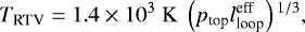 (B.1)
(B.1)
where ptop is the loop-top pressure and  is the effective half-loop length, both of which are measured in the cgs unit. In Figure B.3, as the resolution of the transition region increases, the numerical value monotonically approaches the RTV-predicted value. We note that the deviation of the results of the simulation from those of the RTV prediction is not necessarily evidence of inaccuracy, although, as a general trend, a higher resolution of the transition region should lead to a value closer to the RTV prediction. Deviations from the RTV value in a low-resolution run is prominent at higher coronal temperatures. However, it remains to be seen if the large discrepancy from the RTV value at high coronal temperatures is due to the large numerical diffusion at the transition region or the increase in the required resolution. The coronal-temperature dependence of the transition-region problem should be investigated in the future.
 |
Fig. B.3 Comparison of the time-averaged loop-top temperature Ttop and the loop-top temperature predicted by the RTV scaling law TRTV. |
Finally, we note that there are physical mechanisms that can produce the broadening of the transition region, including ambipolar diffusion (Fontenla et al. 1990; Lanzafame 1995). The transition-region problem should also be revisited considering the additional diffusive processes in future.
Appendix C XUV spectrum from different atmospheric layers
The XUV photons of a specific wavelength (band) do not originate from the plasma with a specific temperature. Indeed, narrow-band filters in the Atmospheric Imaging Assembly of the Solar Dynamics Observatory have broad response functions in terms of temperature (Boerner et al. 2012). Although there is no direct correlation between temperatureand wavelength, it is still useful to understand the energy spectrum emanating from plasma with a specific temperature.
Figure C.1 shows the correlation between the emission measure distribution in a given temperature bin (top panel) and the corresponding spectral energy flux normalised at 1 au (bottom panel) for the fiducial case (f* = 0.01, lloop = 20 Mm). For better visualisation, the spectral energy fluxes averaged over 10 Å are shown in the bottom panel. The black dotted line in the top panel represents the total emission measure distribution, while the black dottedline represents the corresponding spectral energy flux in the bottom panel. We consider three temperature bins centred on T =104 K, T =105 K, and T =106 K corresponding to the upperchromosphere, transition region, and corona, respectively. The corresponding spectral energy fluxes are highlighted with the same colours in the bottom panel, which showcase the following three properties. First, emissions from the upper chromosphere (T ≈ 104 K) dominate the Lyman continuum but negligible in ≤ 600 Å. Second, emissions from the transition region (T ≈ 105 K) are nearly uniform in the middle of the EUV wavelength (200 Å ≤ λ ≤ 800 Å) but negligible in the X-ray range. Third, emissions from the corona (T ≈ 106 K) are the dominant sources of stellar X-rays. The contribution to the EUV emission is also non-negligible, especially in the shorter wavelength.
 |
Fig. C.1 Emission measure in the limited range of temperature and corresponding spectral energy flux at 1 au. For better visualisation, the spectral energy fluxes in the bottom panel are averaged over 10 Å. Orange, green and blue lines correspond to the emission measures and spectral energy fluxes of T ≈ 104 K (chromosphere), T ≈ 105 K (transition region) and T ≈ 106 K (corona), respectively. Black dotted lines show the full emission measure distribution and corresponding full spectral energy flux. |
As a general trend, the low-energy photons tend to originate from the low-temperature plasma and vice versa. We note that a non-negligible fraction of EUV photons originates from the chromosphere and the transition region, and therefore including them in the model is essential in predicting the XUV spectrum.
References
- Airapetian, V. S., Glocer, A., Khazanov, G. V., et al. 2017, ApJ, 836, L3 [NASA ADS] [CrossRef] [Google Scholar]
- Airapetian, V. S., Jin, M., Lueftinger, T., et al. 2021, ApJ, 916, 96 [NASA ADS] [CrossRef] [Google Scholar]
- Alfvén, H. 1947, MNRAS, 107, 211 [CrossRef] [Google Scholar]
- Alvarado-Gómez, J. D., Hussain, G. A. J., Cohen, O., et al. 2016, A&A, 588, A28 [NASA ADS] [CrossRef] [EDP Sciences] [Google Scholar]
- An, C. H., Musielak, Z. E., Moore, R. L., & Suess, S. T. 1989, ApJ, 345, 597 [NASA ADS] [CrossRef] [Google Scholar]
- Antiochos, S. K., & Sturrock, P. A. 1978, ApJ, 220, 1137 [NASA ADS] [CrossRef] [Google Scholar]
- Antiochos, S. K., MacNeice, P. J., Spicer, D. S., & Klimchuk, J. A. 1999, ApJ, 512, 985 [Google Scholar]
- Antolin, P., & Shibata, K. 2010, ApJ, 712, 494 [NASA ADS] [CrossRef] [Google Scholar]
- Antolin, P., Okamoto, T. J., De Pontieu, B., et al. 2015, ApJ, 809, 72 [Google Scholar]
- Antolin, P., Pagano, P., Testa, P., Petralia, A., & Reale, F. 2021, Nat. Astron., 5, 54 [NASA ADS] [CrossRef] [Google Scholar]
- Aschwanden, M. J., & Parnell, C. E. 2002, ApJ, 572, 1048 [NASA ADS] [CrossRef] [Google Scholar]
- Avrett, E. H., & Loeser, R. 2008, ApJS, 175, 229 [Google Scholar]
- Barnes, S. A. 2003, ApJ, 586, 464 [Google Scholar]
- Berghmans, D., Auchère, F., Long, D. M., et al. 2021, A&A, 656, L4 [NASA ADS] [CrossRef] [EDP Sciences] [Google Scholar]
- Bochanski, J. J., Hawley, S. L., Covey, K. R., et al. 2010, AJ, 139, 2679 [NASA ADS] [CrossRef] [Google Scholar]
- Boerner, P., Edwards, C., Lemen, J., et al. 2012, Sol. Phys., 275, 41 [Google Scholar]
- Bonfils, X., Delfosse, X., Udry, S., et al. 2013, A&A, 549, A109 [NASA ADS] [CrossRef] [EDP Sciences] [Google Scholar]
- Bradshaw, S. J., & Cargill, P. J. 2013, ApJ, 770, 12 [NASA ADS] [CrossRef] [Google Scholar]
- Cassak, P. A., Mullan, D. J., & Shay, M. A. 2008, ApJ, 676, L69 [NASA ADS] [CrossRef] [Google Scholar]
- Chamberlin, P. C., Woods, T. N., Crotser, D. A., et al. 2009, Geophys. Res. Lett., 36, L05102 [CrossRef] [Google Scholar]
- Chandran, B. D. G., & Perez, J. C. 2019, J. Plasma Phys., 85, 905850409 [NASA ADS] [CrossRef] [Google Scholar]
- Chen, Y., Przybylski, D., Peter, H., et al. 2021, A&A, 656, L7 [NASA ADS] [CrossRef] [EDP Sciences] [Google Scholar]
- Chitta, L. P., van Ballegooijen, A. A., Rouppe van der Voort, L., DeLuca, E. E., & Kariyappa, R. 2012, ApJ, 752, 48 [Google Scholar]
- Cho, J., & Lazarian, A. 2003, MNRAS, 345, 325 [NASA ADS] [CrossRef] [Google Scholar]
- Cho, J., & Vishniac, E. T. 2000, ApJ, 539, 273 [CrossRef] [Google Scholar]
- Cirtain, J. W., Golub, L., Winebarger, A. R., et al. 2013, Nature, 493, 501 [NASA ADS] [CrossRef] [Google Scholar]
- Claire, M. W., Sheets, J., Cohen, M., et al. 2012, ApJ, 757, 95 [Google Scholar]
- Cranmer, S. R. 2008, ApJ, 689, 316 [NASA ADS] [CrossRef] [Google Scholar]
- Cranmer, S. R. 2009, ApJ, 706, 824 [Google Scholar]
- Cranmer, S. R. 2017, ApJ, 840, 114 [NASA ADS] [CrossRef] [Google Scholar]
- Cranmer, S. R., & van Ballegooijen, A. A. 2005, ApJS, 156, 265 [Google Scholar]
- Dahlburg, R. B., Einaudi, G., Taylor, B. D., et al. 2016, ApJ, 817, 47 [NASA ADS] [CrossRef] [Google Scholar]
- Del Zanna, G., Dere, K. P., Young, P. R., & Landi, E. 2021, ApJ, 909, 38 [NASA ADS] [CrossRef] [Google Scholar]
- De Pontieu, B., McIntosh, S. W., Carlsson, M., et al. 2007, Science, 318, 1574 [Google Scholar]
- Dere, K. P., Landi, E., Mason, H. E., Monsignori Fossi, B. C., & Young, P. R. 1997, A&AS, 125, 149 [NASA ADS] [CrossRef] [EDP Sciences] [Google Scholar]
- Diamond-Lowe, H., Youngblood, A., Charbonneau, D., et al. 2021, AJ, 162, 10 [NASA ADS] [CrossRef] [Google Scholar]
- Dmitruk, P., Matthaeus, W. H., Milano, L. J., et al. 2002, ApJ, 575, 571 [NASA ADS] [CrossRef] [Google Scholar]
- Dressing, C. D., & Charbonneau, D. 2015, ApJ, 807, 45 [Google Scholar]
- Duvvuri, G. M., Pineda, J. S., Berta-Thompson, Z. K., et al. 2021, ApJ, 913, 40 [NASA ADS] [CrossRef] [Google Scholar]
- Edlén, B. 1943, ZAp, 22, 30 [Google Scholar]
- Ehrenreich, D., Bourrier, V., Wheatley, P. J., et al. 2015, Nature, 522, 459 [Google Scholar]
- Einaudi, G., Velli, M., Politano, H., & Pouquet, A. 1996, ApJ, 457, L113 [NASA ADS] [Google Scholar]
- Felipe, T., Kuckein, C., & Thaler, I. 2018, A&A, 617, A39 [NASA ADS] [CrossRef] [EDP Sciences] [Google Scholar]
- Fontenla, J. M., Avrett, E. H., & Loeser, R. 1990, ApJ, 355, 700 [NASA ADS] [CrossRef] [Google Scholar]
- France, K., Arulanantham, N., Fossati, L., et al. 2018, ApJS, 239, 16 [Google Scholar]
- Galsgaard, K., & Nordlund, Å. 1996, J. Geophys. Res., 101, 13445 [NASA ADS] [CrossRef] [Google Scholar]
- Goodman, M. L., & Judge, P. G. 2012, ApJ, 751, 75 [NASA ADS] [CrossRef] [Google Scholar]
- Gorti, U., & Hollenbach, D. 2009, ApJ, 690, 1539 [Google Scholar]
- Gottlieb, S., Shu, C.-W., & Tadmor, E. 2001, SIAM Rev., 43, 89 [NASA ADS] [CrossRef] [Google Scholar]
- Güdel, M., Guinan, E. F., & Skinner, S. L. 1997, ApJ, 483, 947 [Google Scholar]
- Güdel, M., Audard, M., Kashyap, V. L., Drake, J. J., & Guinan, E. F. 2003, ApJ, 582, 423 [Google Scholar]
- Gudiksen, B. V., & Nordlund, Å. 2005, ApJ, 618, 1020 [NASA ADS] [CrossRef] [Google Scholar]
- Guinan, E. F., Engle, S. G., & Durbin, A. 2016, ApJ, 821, 81 [NASA ADS] [CrossRef] [Google Scholar]
- Günther, H. M., Schmitt, J. H. M. M., Robrade, J., & Liefke, C. 2007, A&A, 466, 1111 [NASA ADS] [CrossRef] [EDP Sciences] [Google Scholar]
- Hansteen, V., Guerreiro, N., De Pontieu, B., & Carlsson, M. 2015, ApJ, 811, 106 [NASA ADS] [CrossRef] [Google Scholar]
- Heyvaerts, J., & Priest, E. R. 1983, A&A, 117, 220 [NASA ADS] [Google Scholar]
- Hollweg, J. V. 1984, Sol. Phys., 91, 269 [CrossRef] [Google Scholar]
- Hollweg, J. V., & Yang, G. 1988, J. Geophys. Res., 93, 5423 [Google Scholar]
- Hollweg, J. V., Jackson, S., & Galloway, D. 1982, Sol. Phys., 75, 35 [NASA ADS] [CrossRef] [Google Scholar]
- Hood, A. W., Brooks, S. J., & Wright, A. N. 2002, Proc. Roy. Soc. London Ser. A, 458, 2307 [NASA ADS] [CrossRef] [Google Scholar]
- Hossain, M., Gray, P. C., Pontius, et al. 1995, Physics of Fluids, 7, 2886 [NASA ADS] [CrossRef] [Google Scholar]
- Hunter, J. D. 2007, Computi. Sci. Eng., 9, 90 [NASA ADS] [CrossRef] [Google Scholar]
- Iijima, H. 2016, PhD thesis, The University of Tokyo, Japan [Google Scholar]
- Iijima, H., & Imada, S. 2021, ApJ, 917, 65 [NASA ADS] [CrossRef] [Google Scholar]
- Ionson, J. A. 1978, ApJ, 226, 650 [NASA ADS] [CrossRef] [Google Scholar]
- Irwin, J., & Bouvier, J. 2009, IAU Symp., 258, 363 [Google Scholar]
- Ishikawa, S.-n., Glesener, L., Krucker, S., et al. 2017, Nat. Astron., 1, 771 [Google Scholar]
- Ishikawa, R., Trujillo Bueno, J., del Pino Aleman, T., et al. 2021, Sci. Adv., 7, eabe8406 [NASA ADS] [CrossRef] [Google Scholar]
- Jess, D. B., Reznikova, V. E., Ryans, R. S. I., et al. 2016, Nat. Phys., 12, 179 [NASA ADS] [CrossRef] [Google Scholar]
- Johnston, C. D., & Bradshaw, S. J. 2019, ApJ, 873, L22 [NASA ADS] [CrossRef] [Google Scholar]
- Johnston, C. D., Hood, A. W., Cargill, P. J., & De Moortel, I. 2017, A&A, 597, A81 [NASA ADS] [CrossRef] [EDP Sciences] [Google Scholar]
- Johnston, C. D., Hood, A. W., De Moortel, I., Pagano, P., & Howson, T. A. 2021, A&A, 654, A2 [NASA ADS] [CrossRef] [EDP Sciences] [Google Scholar]
- Johnstone, C. P., & Güdel, M. 2015, A&A, 578, A129 [NASA ADS] [CrossRef] [EDP Sciences] [Google Scholar]
- Johnstone, C. P., Bartel, M., & Güdel, M. 2021, A&A, 649, A96 [EDP Sciences] [Google Scholar]
- Judge, P. G., Solomon, S. C., & Ayres, T. R. 2003, ApJ, 593, 534 [NASA ADS] [CrossRef] [Google Scholar]
- Kanella, C., & Gudiksen, B. V. 2018, A&A, 617, A50 [NASA ADS] [CrossRef] [EDP Sciences] [Google Scholar]
- Katsukawa, Y., & Tsuneta, S. 2005, ApJ, 621, 498 [NASA ADS] [CrossRef] [Google Scholar]
- Kawaler, S. D. 1988, ApJ, 333, 236 [Google Scholar]
- Keller, C. U., Schüssler, M., Vögler, A., & Zakharov, V. 2004, ApJ, 607, L59 [NASA ADS] [CrossRef] [Google Scholar]
- Klimchuk, J. A. 2006, Sol. Phys., 234, 41 [Google Scholar]
- Klimchuk, J. A., Lemen, J. R., Feldman, U., Tsuneta, S., & Uchida, Y. 1992, PASJ, 44, L181 [NASA ADS] [CrossRef] [Google Scholar]
- Klimchuk, J. A., Patsourakos, S., & Cargill, P. J. 2008, ApJ, 682, 1351 [Google Scholar]
- Kochukhov, O., Hackman, T., Lehtinen, J. J., & Wehrhahn, A. 2020, A&A, 635, A142 [NASA ADS] [CrossRef] [EDP Sciences] [Google Scholar]
- Kraft, R. P. 1967, ApJ, 150, 551 [Google Scholar]
- Kudoh, T., & Shibata, K. 1999, ApJ, 514, 493 [NASA ADS] [CrossRef] [Google Scholar]
- Lanzafame, A. C. 1995, A&A, 302, 839 [NASA ADS] [Google Scholar]
- Lecavelier des Etangs, A., Bourrier, V., Wheatley, P. J., et al. 2012, A&A, 543, L4 [NASA ADS] [CrossRef] [EDP Sciences] [Google Scholar]
- Lemen, J. R., Title, A. M., Akin, D. J., et al. 2012, Sol. Phys., 275, 17 [Google Scholar]
- Linsky, J. L., Fontenla, J., & France, K. 2014, ApJ, 780, 61 [Google Scholar]
- Magaudda, E., Stelzer, B., Covey, K. R., et al. 2020, A&A, 638, A20 [NASA ADS] [CrossRef] [EDP Sciences] [Google Scholar]
- Malanushenko, A., Cheung, M. C. M., DeForest, C. E., Klimchuk, J. A., & Rempel, M. 2021, ApJ, submitted [arXiv:2106.14877] [Google Scholar]
- Matsumoto, T., & Shibata, K. 2010, ApJ, 710, 1857 [NASA ADS] [CrossRef] [Google Scholar]
- Matt, S. P., Brun, A. S., Baraffe, I., Bouvier, J., & Chabrier, G. 2015, ApJ, 799, L23 [Google Scholar]
- Matthaeus, W. H., Zank, G. P., Oughton, S., Mullan, D. J., & Dmitruk, P. 1999, ApJ, 523, L93 [NASA ADS] [CrossRef] [Google Scholar]
- McIntosh, S. W., de Pontieu, B., Carlsson, M., et al. 2011, Nature, 475, 477 [Google Scholar]
- Meyer, C. D., Balsara, D. S., & Aslam, T. D. 2012, MNRAS, 422, 2102 [NASA ADS] [CrossRef] [Google Scholar]
- Meyer, C. D., Balsara, D. S., & Aslam, T. D. 2014, J. Comput. Phys., 257, 594 [NASA ADS] [CrossRef] [Google Scholar]
- Miyoshi, T., & Kusano, K. 2005, J. Comput. Phys., 208, 315 [NASA ADS] [CrossRef] [Google Scholar]
- Moriyasu, S., Kudoh, T., Yokoyama, T., & Shibata, K. 2004, ApJ, 601, L107 [NASA ADS] [CrossRef] [Google Scholar]
- Nakariakov, V. M., & Ofman, L. 2001, A&A, 372, L53 [NASA ADS] [CrossRef] [EDP Sciences] [Google Scholar]
- Nakatani, R., Hosokawa, T., Yoshida, N., Nomura, H., & Kuiper, R. 2018, ApJ, 865, 75 [Google Scholar]
- Okamoto, T. J., Antolin, P., De Pontieu, B., et al. 2015, ApJ, 809, 71 [NASA ADS] [CrossRef] [Google Scholar]
- Oran, R., Landi, E., van der Holst, B., Sokolov, I. V., & Gombosi, T. I. 2017, ApJ, 845, 98 [CrossRef] [Google Scholar]
- Osterbrock, D. E. 1961, ApJ, 134, 347 [NASA ADS] [CrossRef] [Google Scholar]
- Owen, J. E., & Wu, Y. 2013, ApJ, 775, 105 [Google Scholar]
- Pagano, P., & De Moortel, I. 2019, A&A, 623, A37 [NASA ADS] [CrossRef] [EDP Sciences] [Google Scholar]
- Pallavicini, R., Golub, L., Rosner, R., et al. 1981, ApJ, 248, 279 [NASA ADS] [CrossRef] [Google Scholar]
- Parker, E. N. 1972, ApJ, 174, 499 [NASA ADS] [CrossRef] [Google Scholar]
- Parker, E. N. 1983, ApJ, 264, 642 [Google Scholar]
- Parker, E. N. 1988, ApJ, 330, 474 [Google Scholar]
- Peres, G., Serio, S., Vaiana, G. S., & Rosner, R. 1982, ApJ, 252, 791 [NASA ADS] [CrossRef] [Google Scholar]
- Pesnell, W. D., Thompson, B. J., & Chamberlin, P. C. 2012, Sol. Phys., 275, 3 [Google Scholar]
- Pevtsov, A. A., Fisher, G. H., Acton, L. W., et al. 2003, ApJ, 598, 1387 [Google Scholar]
- Pizzolato, N., Maggio, A., Micela, G., Sciortino, S., & Ventura, P. 2003, A&A, 397, 147 [NASA ADS] [CrossRef] [EDP Sciences] [Google Scholar]
- Priest, E. 2014, Magnetohydrodynamics of the Sun (Cambridge: Cambridge University Press) [Google Scholar]
- Rappazzo, A. F., Velli, M., Einaudi, G., & Dahlburg, R. B. 2007, ApJ, 657, L47 [Google Scholar]
- Rappazzo, A. F., Velli, M., Einaudi, G., & Dahlburg, R. B. 2008, ApJ, 677, 1348 [Google Scholar]
- Reale, F., & Micela, G. 1998, A&A, 334, 1028 [NASA ADS] [Google Scholar]
- Reale, F., Güdel, M., Peres, G., & Audard, M. 2004, A&A, 416, 733 [NASA ADS] [CrossRef] [EDP Sciences] [Google Scholar]
- Reiners, A., Basri, G., & Browning, M. 2009, ApJ, 692, 538 [NASA ADS] [CrossRef] [Google Scholar]
- Rempel, M. 2017, ApJ, 834, 10 [Google Scholar]
- Ribas, I., Guinan, E. F., Güdel, M., & Audard, M. 2005, ApJ, 622, 680 [Google Scholar]
- Rosner, R., Tucker, W. H., & Vaiana, G. S. 1978, ApJ, 220, 643 [Google Scholar]
- Rumph, T., Bowyer, S., & Vennes, S. 1994, AJ, 107, 2108 [NASA ADS] [CrossRef] [Google Scholar]
- Rybicki, G. B., & Lightman, A. P. 1979, Radiative Processes in Astrophysics (Hoboken: Wiley-VCH) [Google Scholar]
- Saar, S. H. 1996, in Stellar Surface Structure, eds. K. G. Strassmeier, & J. L. Linsky (Berlin: Springer), 176, 237 [NASA ADS] [Google Scholar]
- Saar, S. H. 2001, ASP Conf. Ser., 223, 292 [NASA ADS] [Google Scholar]
- Sakurai, T., Goossens, M., & Hollweg, J. V. 1991, Sol. Phys., 133, 227 [Google Scholar]
- Sanz-Forcada, J., Micela, G., Ribas, I., et al. 2011, A&A, 532, A6 [NASA ADS] [CrossRef] [EDP Sciences] [Google Scholar]
- Scelsi, L., Maggio, A., Peres, G., & Pallavicini, R. 2005, A&A, 432, 671 [NASA ADS] [CrossRef] [EDP Sciences] [Google Scholar]
- Schmelz, J. T., Reames, D. V., von Steiger, R., & Basu, S. 2012, ApJ, 755, 33 [NASA ADS] [CrossRef] [Google Scholar]
- Schrijver, C. J., van den Oord, G. H. J., & Mewe, R. 1994, A&A, 289, L23 [NASA ADS] [Google Scholar]
- See, V., Matt, S. P., Folsom, C. P., et al. 2019, ApJ, 876, 118 [Google Scholar]
- Serio, S., Peres, G., Vaiana, G. S., Golub, L., & Rosner, R. 1981, ApJ, 243, 288 [NASA ADS] [CrossRef] [Google Scholar]
- Shebalin, J. V., Matthaeus, W. H., & Montgomery, D. 1983, J. Plasma Phys., 29, 525 [Google Scholar]
- Shibata, K., & Yokoyama, T. 2002, ApJ, 577, 422 [CrossRef] [Google Scholar]
- Shimizu, T. 1995, PASJ, 47, 251 [NASA ADS] [Google Scholar]
- Shoda, M., Yokoyama, T., & Suzuki, T. K. 2018, ApJ, 853, 190 [Google Scholar]
- Shoda, M., Suzuki, T. K., Asgari-Targhi, M., & Yokoyama, T. 2019, ApJ, 880, L2 [Google Scholar]
- Shoda, M., Suzuki, T. K., Matt, S. P., et al. 2020, ApJ, 896, 123 [Google Scholar]
- Shu, C.-W., & Osher, S. 1988, J. Comput. Phys., 77, 439 [NASA ADS] [CrossRef] [Google Scholar]
- Skumanich, A. 1972, ApJ, 171, 565 [Google Scholar]
- Spitzer, L., & Härm, R. 1953, Phys. Rev., 89, 977 [Google Scholar]
- Spruit, H. C., & Zweibel, E. G. 1979, Sol. Phys., 62, 15 [NASA ADS] [CrossRef] [Google Scholar]
- Sreejith, A. G., Fossati, L., Youngblood, A., France, K., & Ambily, S. 2020, A&A, 644, A67 [NASA ADS] [CrossRef] [EDP Sciences] [Google Scholar]
- Srivastava, A. K., Shetye, J., Murawski, K., et al. 2017, Sci. Rep., 7, 43147 [Google Scholar]
- Stein, R. F. 1971, ApJS, 22, 419 [Google Scholar]
- Steiner, O., Grossmann-Doerth, U., Knölker, M., & Schüssler, M. 1998, ApJ, 495, 468 [NASA ADS] [CrossRef] [Google Scholar]
- Sturrock, P. A., & Uchida, Y. 1981, ApJ, 246, 331 [NASA ADS] [CrossRef] [Google Scholar]
- Suresh, A., & Huynh, H. T. 1997, J. Comput. Phys., 136, 83 [Google Scholar]
- Suzuki, T. K., & Inutsuka, S.-i. 2005, ApJ, 632, L49 [NASA ADS] [CrossRef] [Google Scholar]
- Takasao, S., Isobe, H., & Shibata, K. 2013, PASJ, 65, 62 [Google Scholar]
- Takasao, S., Mitsuishi, I., Shimura, T., et al. 2020, ApJ, 901, 70 [NASA ADS] [CrossRef] [Google Scholar]
- Telleschi, A., Güdel, M., Briggs, K., et al. 2005, ApJ, 622, 653 [Google Scholar]
- Testa, P., De Pontieu, B., Allred, J., et al. 2014, Science, 346, 1255724 [Google Scholar]
- Toriumi, S., Airapetian, V. S., Hudson, H. S., et al. 2020, ApJ, 902, 36 [CrossRef] [Google Scholar]
- Tsuneta, S., Ichimoto, K., Katsukawa, Y., et al. 2008, ApJ, 688, 1374 [Google Scholar]
- Tu, L., Johnstone, C. P., Güdel, M., & Lammer, H. 2015, A&A, 577, L3 [NASA ADS] [CrossRef] [EDP Sciences] [Google Scholar]
- van Ballegooijen, A. A. 1986, ApJ, 311, 1001 [NASA ADS] [CrossRef] [Google Scholar]
- van Ballegooijen, A. A., & Asgari-Targhi, M. 2017, ApJ, 835, 10 [CrossRef] [Google Scholar]
- van Ballegooijen, A. A., Asgari-Targhi, M., Cranmer, S. R., & DeLuca, E. E. 2011, ApJ, 736, 3 [Google Scholar]
- Van Damme, H. J., De Moortel, I., Pagano, P., & Johnston, C. D. 2020, A&A, 635, A174 [NASA ADS] [CrossRef] [EDP Sciences] [Google Scholar]
- van der Holst, B., Sokolov, I. V., Meng, X., et al. 2014, ApJ, 782, 81 [Google Scholar]
- van der Walt, S., Colbert, S. C., & Varoquaux, G. 2011, Comput. Sci. Eng., 13, 22 [Google Scholar]
- Van Kooten, S. J., & Cranmer, S. R. 2017, ApJ, 850, 64 [NASA ADS] [CrossRef] [Google Scholar]
- van Leer, B. 1979, J. Comput. Phys., 32, 101 [Google Scholar]
- Vasquez, B. J. 1990, ApJ, 356, 693 [CrossRef] [Google Scholar]
- Verdini, A., & Velli, M. 2007, ApJ, 662, 669 [Google Scholar]
- Verdini, A., Grappin, R., & Velli, M. 2012, A&A, 538, A70 [NASA ADS] [CrossRef] [EDP Sciences] [Google Scholar]
- Verdini, A., Grappin, R., & Montagud-Camps, V. 2019, Sol. Phys., 294, 65 [Google Scholar]
- Verwichte, E., Nakariakov, V. M., Ofman, L., & Deluca, E. E. 2004, Sol. Phys., 223, 77 [Google Scholar]
- Vidal-Madjar, A., Lecavelier des Etangs, A., Désert, J. M., et al. 2003, Nature, 422, 143 [Google Scholar]
- Vidotto, A. A., Gregory, S. G., Jardine, M., et al. 2014, MNRAS, 441, 2361 [Google Scholar]
- Wang, Y. M. 2020, ApJ, 904, 199 [NASA ADS] [CrossRef] [Google Scholar]
- Wang, L., Bai,X.-N., & Goodman, J. 2019, ApJ, 874, 90 [NASA ADS] [CrossRef] [Google Scholar]
- Washinoue, H., & Suzuki, T. K. 2019, ApJ, 885, 164 [NASA ADS] [CrossRef] [Google Scholar]
- Weber, E. J., & Davis, Leverett, J. 1967, ApJ, 148, 217 [Google Scholar]
- Winters, J. G., Henry, T. J., Jao, W.-C., et al. 2019, AJ, 157, 216 [NASA ADS] [CrossRef] [Google Scholar]
- Withbroe, G. L., & Noyes, R. W. 1977, ARA&A, 15, 363 [Google Scholar]
- Woods, T. N., Chamberlin, P. C., Harder, J. W., et al. 2009, Geophys. Res. Lett., 36, L01101 [NASA ADS] [CrossRef] [Google Scholar]
- Wright, N. J.,& Drake, J. J. 2016, Nature, 535, 526 [NASA ADS] [CrossRef] [Google Scholar]
- Wright, N. J., Drake, J. J., Mamajek, E. E., & Henry, G. W. 2011, ApJ, 743, 48 [Google Scholar]
- Wright, N. J., Newton, E. R., Williams, P. K. G., Drake, J. J., & Yadav, R. K. 2018, MNRAS, 479, 2351 [Google Scholar]
- Youngblood, A., France, K., Loyd, R. O. P., et al. 2017, ApJ, 843, 31 [Google Scholar]
- Zhuleku, J., Warnecke, J., & Peter, H. 2020, A&A, 640, A119 [NASA ADS] [CrossRef] [EDP Sciences] [Google Scholar]
All Tables
List of the simulation runs executed to study the transition-region problem. We note that Δsmin corresponds to the spatial resolution of the transition region.
All Figures
|
Fig. 1 Schematic picture of the system. One-dimensional dynamics along the axis of the closed flux tube is simulated. The axis isindicated by the dotted line, while the flux tube surface is denoted by green lines. The flux tube is intended to be nearly vertical and super-radially expanding. The geometry of the loop is defined by the filling factor f and radial distance r as functions of field-aligned distance s. |
| In the text | |
|
Fig. 2 Shape of the flux-tube axis defined by Eq. (7). x and z denote the horizontal and vertical coordinates, respectively. |
| In the text | |
|
Fig. 3 Effective and original optically thin radiative loss functions, Λeff(T) and Λ(T), shown with solid and dashed lines, respectively. Also shown, by crosses, are the loss function from the CHIANTI atomic database with photospheric abundance. |
| In the text | |
|
Fig. 4 Simulated loop properties of the fiducial case. Top: time-averaged (solid line) and snapshot (dashed line) profiles of mass density along the loop axis. Middle: time-averaged (solid line) and snapshot (dashed line) profiles of temperature along the loop axis. Bottom: time-averaged differential emission measure (solid line). Annotations ‘TR’ in the middle panel indicate the locations of the transition region in the snapshot profile. |
| In the text | |
|
Fig. 5 Observed (blue) and simulated (red) spectral flux density of the Sun measured at 1 au. The observed spectrum is retrieved in the solar activity minimum. The two spectra are in a good agreement below the Lyman edge (≤912 Å). |
| In the text | |
|
Fig. 6 Coronal-property dependences on the effective loop length. Top: relation between the effective half loop length
|
| In the text | |
|
Fig. 7 Relation between the coronal conductive flux and loop length. Top: half loop length versus coronal conductive flux measured at Tave = 106 K (red circles) and averaged in 10 Mm ≤ s ≤ 15 Mm (blue diamonds). Also shown, by the solid line, is the power-law fitting to the blue diamonds. Bottom: same as the top panel but with respect to the effective half loop length
|
| In the text | |
|
Fig. 8 (Effective) loop length versus X-ray luminosity LX (red circles) and EUV luminosity LEUV (blue diamonds). The solid and dashed lines show the power-law fittings to the simulation results. The top and bottom panels show the relation with respect to the half loop length lloop and the effective hal loop length |
| In the text | |
|
Fig. 9 Magnetic filling factor on the photosphere f* versus time-averaged loop-top temperature (Ttop, top panel) and loop-top electron density (ne,top, bottom panel). The half loop length is fixed to lloop = 20 Mm. Red circles show the simulation results and the solid lines show the power-law fittings to them. |
| In the text | |
|
Fig. 10 Relation between filling factor and coronal conductive flux. Top: magnetic filling factor on the photosphere f* versus backward conductive flux measured in the corona. The half loop length is fixed to lloop =20 Mm. The red circles and blue diamonds represent the flux measured at Tave = 106 K and averaged in 10 Mm ≤ s ≤ 15 Mm. The black solid line is the power-law fitting to the blue diamonds. Bottom: same as the top panel but the vertical axis denotes |
| In the text | |
|
Fig. 11 Filling-factor dependence of the XUV spectrum. Left: spectral energy flux at 1 au for f* = 0.01 (orange, solid), f* = 0.1 (green, dashed), and f* = 1 (blue, dotted). Centre: energy-flux ratio of f* = 1 to f* =0.01. Right: photon-number luminosity spectrum for f* = 0.01 (orange, solid), f* = 0.1 (green, dashed), and f* = 1 (blue, dotted). Bottom panels are the same as top panels but with logarithmic x axis thatemphasise the short-wavelength region. For better visualisation, spectra are averaged over 20 Å-bins in the top panels. |
| In the text | |
|
Fig. 12 Unsigned magnetic flux |
| In the text | |
|
Fig. 13 Magnetic filling factor on the photosphere f* versus photon number luminosity in the EUV range. Each simulation run corresponds to each red circle. The black solid line shows the power-law fitting to the simulation results. |
| In the text | |
|
Fig. 14 Inferred relations between X-ray luminosity and EUV emission. Top: correlation between the X-ray luminosity LX and EUV luminosity LEUV. X-ray and EUV are defined in terms of wavelength λ as 5 Å < λ ≤ 100 Å and 100 Å < λ ≤ 912 Å, respectively. Each black circle corresponds to the simulation run listed in Table 2, and the black solid line shows the power-law fitting to them. Also shown, by the red points with vertical error bars, are the empirical estimation by Sanz-Forcada et al. (2011). Bottom: same as the top panel but for the X-ray luminosity
LX and photon number luminosity |
| In the text | |
|
Fig. 15 Model of Alfvén-wave transmission across a free boundary with density jump. |
| In the text | |
|
Fig. 16 Half loop length versus timescale of Alfvén-wave crossing (τA red circles) and Alfvén-wave turbulent dissipation (τdiss, blue diamonds). For the definitions of τA and τdiss, see Eq. (110). |
| In the text | |
|
Fig. 17 Rossby number versus normalised X-ray luminosity (blue diamonds). The Rossby number and the filling factor are connected by Eq. (118). Results for the fixed half loop length lloop =20 Mm are shown. Also shown, by the solid and dashed lines, are the observational relation by Pizzolato et al. (2003) and its scaled-down version (1/8). |
| In the text | |
|
Fig. B.1 Time evolution of the loop-top electron density ne,top (top panel) and temperature Ttop (bottom panel) for fixed filling factor f* = 0.05 and half loop length lloop = 20 Mm. Three lines show the results with Δsmin = 5 km and HLL solver (red), Δsmin = 5 km and HLLD solver (green), and Δsmin = 2 km and HLLD solver (blue), respectively. |
| In the text | |
|
Fig. B.2 Same as Figure B.1 but for f* = 1 and lloop = 20 Mm. |
| In the text | |
|
Fig. B.3 Comparison of the time-averaged loop-top temperature Ttop and the loop-top temperature predicted by the RTV scaling law TRTV. |
| In the text | |
|
Fig. C.1 Emission measure in the limited range of temperature and corresponding spectral energy flux at 1 au. For better visualisation, the spectral energy fluxes in the bottom panel are averaged over 10 Å. Orange, green and blue lines correspond to the emission measures and spectral energy fluxes of T ≈ 104 K (chromosphere), T ≈ 105 K (transition region) and T ≈ 106 K (corona), respectively. Black dotted lines show the full emission measure distribution and corresponding full spectral energy flux. |
| In the text | |
Current usage metrics show cumulative count of Article Views (full-text article views including HTML views, PDF and ePub downloads, according to the available data) and Abstracts Views on Vision4Press platform.
Data correspond to usage on the plateform after 2015. The current usage metrics is available 48-96 hours after online publication and is updated daily on week days.
Initial download of the metrics may take a while.