| Issue |
A&A
Volume 656, December 2021
|
|
|---|---|---|
| Article Number | A86 | |
| Number of page(s) | 12 | |
| Section | The Sun and the Heliosphere | |
| DOI | https://doi.org/10.1051/0004-6361/202141500 | |
| Published online | 07 December 2021 | |
Investigation of the subsurface structure of a sunspot based on the spatial distribution of oscillation centers inferred from umbral flashes⋆
1
Astronomy Program, Department of Physics and Astronomy, Seoul National University, Seoul, 08826
Republic of Korea
e-mail: This email address is being protected from spambots. You need JavaScript enabled to view it.
2
Max Planck Institute for Solar System Research, Justus-von-Liebig-Weg 3, 37077 Göttingen, Germany
Received:
9
June
2021
Accepted:
13
September
2021
Abstract
The subsurface structure of a solar sunspot is important for the stability of the sunspot and the energy transport therein. Two subsurface structure models have been proposed, the monolithic and cluster models, but no clear observational evidence supporting a particular model has been found to date. To obtain clues about the subsurface structure of sunspots, we analyzed umbral flashes in merging sunspots registered by IRIS Mg II 2796 Å slit-jaw images. Umbral flashes are regarded as an observational manifestation of magnetohydrodynamic shock waves originating from convection cells below the photosphere. By tracking the motion of individual umbral flashes, we determined the position of the convection cells that are the oscillation centers located below the umbra. We found that the oscillation centers are preferentially located at dark nuclei in the umbral cores rather than in bright regions such as light bridges or umbral dots. Moreover, the oscillation centers tend to deviate from the convergent interface of the merging sunspots where vigorous convection is expected to occur. We also found that the inferred depths of the convection cells have no noticeable regional dependence. These results suggest that the subsurface of the umbra is an environment where convection can occur more easily than the convergent interface, and hence support the cluster model. For more concrete results, further studies based on umbral velocity oscillations in the lower atmosphere are required.
Key words: sunspots / Sun: chromosphere / Sun: oscillations / Sun: helioseismology
Movie is available at https://www.aanda.org
© ESO 2021
1. Introduction
The subsurface structure of sunspots is an important topic in solar physics. This veiled structure situated below the photosphere should be interacting with convective flows, playing a key role in the formation, evolution, and dissipation of the sunspots. The subsurface structure of sunspots is also important in thermal energy transfer. It determines the intensity of the umbrae and gives an indication of the formation mechanism of the inhomogeneous small-scale structures inside sunspots (Borrero & Ichimoto 2011).
Previous studies have proposed two representative models of the sunspot subsurface structure: the monolithic model (Hoyle 1949) and the cluster model (Parker 1979). The monolithic model treats a sunspot as a single magnetic flux tube. By contrast, in the cluster model, also known as the jellyfish or spaghetti model, a sunspot is considered to be an assembly of small flux tubes. There are several observational and theoretical works to verify each model, but they remain inconclusive.
The early magnetic field measurements of sunspots seemed to support the monolithic model. It is well known that a sunspot has a systematic magnetic field structure (Hoyle 1949) that is characterized by monotonically decreasing field strength and increasing field inclination from the sunspot center toward its boundary; this favors the monolithic model. However, it is reported that the power of the magnetic field strength oscillations has isolated multiple peaks inside sunspots (Rueedi et al. 1998; Balthasar 1999). Each penumbral fibril regarded as a magnetic flux tube shows independent behavior, which is referred to as uncombed penumbra (Thomas & Weiss 2004). These findings hint toward the cluster model rather than the monolithic model.
High resolution observations revealed the existence of subarcsecond structures inside sunspot umbrae that are represented by umbral dots and light bridges. These structures are closely related to convective motions (Ortiz et al. 2010; Watanabe et al. 2012). Initially, it was suggested that they cannot be formed in the strong magnetic field environment due to the inhibition of horizontal motions in plasma convection. They were naturally regarded as a tip of the field-free hot gases between magnetic flux tubes in the cluster models (Parker 1979; Choudhuri 1986). Contrary to this expectation, recent magnetohydrodynamic (MHD) simulations based on the monolithic model have successfully reproduced realistic umbral dots (Schüssler & Vögler 2006) or even the sunspots’ overall fine structures (Rempel 2011). It implies that the magneto-convection, which is the convection of magnetized plasma, can produce tiny field-free regions inside large flux tubes. Accordingly, it still remains debatable whether these small-scale structures are intrusions between small magnetic flux tubes or internal structures of large flux tubes caused by magneto-convection (see Borrero & Ichimoto 2011 and references therein).
Local helioseismology provides information about the physical quantities below the photosphere. One of these quantities is the subsurface converging flow, which is required for the cluster model as it helps individual small flux tubes to keep together. Zhao et al. (2001) reported a converging downflow 1500 to 5000 km below the photospheric surface of a sunspot. On the contrary, Gizon et al. (2009) found a horizontal outflow between the solar surface and the depth of 4500 km. Therefore, further helioseismic works need to be carried out for a solid conclusion.
This debate on the sunspot subsurface structure is also inconclusive in theoretical studies. Meyer et al. (1974) investigated the instability below a sunspot, and conjectured that the small-scale mixing of magnetized and non-magnetized gas will occur below 2000 km, which matches a picture of the monolithic model. On the other hand, Parker (1975) argued that a sunspot below the photosphere cannot be a single magnetic structure due to fluting or interchange instabilities. In conclusion, at present we do not have a solidly established view of the subsurface structure of sunspots.
To resolve this problem, we investigate here the subsurface structure of a sunspot using umbral flashes. Beckers & Tallant (1969) obtained a time series of Ca II K-line filtergrams and found that small regions inside sunspot umbrae often brighten for a short period time; they named this phenomenon umbral flashes. They were later identified with umbral oscillations. Giovanelli (1972) examined the time series of Hα Dopplergrams, and found the oscillations of velocity at fixed points inside sunspot umbrae. It was revealed that these velocity oscillations are upward propagating slow MHD waves (Lites 1984; Centeno et al. 2006). The umbral flashes are now usually understood as a shock, the nonlinear development of the slow MHD waves (Rouppe van der Voort et al. 2003).
We expect that umbral flashes provide information about the wave sources in the interior. These sources may be very relevant to the subsurface structure of a sunspot. Recent studies show that it is possible to estimate the wave sources by analyzing oscillatory phenomena (Zhao et al. 2015; Felipe & Khomenko 2017; Kang et al. 2019; Cho & Chae 2020). It is expected that the wave sources are located between 1000 and 5000 km below the photosphere. If we assume that the waves are generated by convective motions, we can infer the distribution of convection cells below the sunspot photosphere. As we mentioned above, umbral dots or light bridges are considered to be the photospheric signature of the convection. Previous studies reported the observational evidence for the relation between umbral dots in the photosphere and three-minute umbral velocity oscillations at the temperature minimum region (Chae et al. 2017; Cho et al. 2019). It implies that oscillations inside umbrae can be a good tool for investigating the site of the convection below sunspots.
We determine the spatial distribution of convection cells by analyzing the motion of umbral flashes and infer the subsurface structure of the sunspot based on these results. This is similar to the method of finding fault lines or plate boundaries in the Earth’s crust. Seismic waves of an earthquake typically occur near a convergent boundary of plates and are a useful tool for investigating the internal structure of the Earth. We expect that umbral flashes can be used in a similar way to investigate the source of slow MHD waves and ascertain the subsurface structure of sunspots.
2. Hypothesis
An oscillation center is defined as the first detected position of a horizontally propagating oscillation pattern in an umbra (Cho et al. 2019). Observations support the hypothesis that the wave source is located below the oscillation center. Cho & Chae (2020) nicely demonstrate that the observed horizontal pattern of propagation is very much consistent with the picture of generation of the fast MHD waves by a subsurface source and quasi-spherical propagation in the interior. The convective motions are assumed as the physical mechanism of the wave generation (Lee 1993; Moore 1973). Therefore, an oscillation center gives us the spatial information about the convection cell below the sunspot.
It is expected that the wave generation process is different between the two sunspot subsurface structure models. Although it must be magneto-convection that excites waves in both models, the cluster model will generate more waves. The cluster model has field-free region between small flux tubes, whereas the monolithic model does not. The existence of field-free region will facilitate the horizontal motion of plasma, and the wave generation will be easily activated. The main challenge is to determine quantitatively which model can explain the observed wave generation rate in a sunspot.
It is therefore important to establish a comparison target in order to distinguish between the two models. When two sunspots merge and become one, it is possible to identify the remnant interface between the two sunspots as a light bridge for a while even after merging. We call this remnant a convergent interface. This convergent interface is our comparison target. Figure 1 illustrates our hypothesis. Generally, a sunspot has funnel-shaped field lines. Thus, when two sunspots are merging, a field-free cusp structure forms on the convergent interface, and is observed as a light bridge in the photosphere. The cusp structure may be maintained for a while even after the end of the merging process at the photosphere. The cusp structures in both models certainly resemble the field-free region in the cluster model. In the monolithic model (Fig. 1a) it is thus expected that more waves will be generated in the cusp structure rather than in the large flux tube. This will cause more oscillation centers to occur near the convergent interface than on the umbral cores (Fig. 1b). If the subsurface structure of the sunspot is close to the cluster model, on the contrary, the cusp structure can be considered one of the many field-free gaps (Fig. 1c). Therefore, the oscillation centers will be found regardless of the convergent interface position (Fig. 1d). Hence, the spatial distribution of oscillation centers in relation to the convergent interface serves as a useful observational basis to determine which model is more plausible.
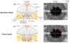 |
Fig. 1. Schematic representation of the hypothesis of this study. Left: cross sections of two merging sunspots in (a) the monolithic model and (c) the cluster model. The black solid arrows indicate magnetic field lines. The yellow region is a magnetic field-free region. The vertical dashed line indicates the convergent interface. The red circular arrows indicate the general convection cells. The opaque red circular arrows indicate the magneto-convection cells. Right: distributions of the oscillation centers on the plane of the sky (panels b and d). The oscillation centers are indicated with red concentric circles. |
3. Data and analysis
For the present study we used data taken by the Interface Region Imaging Spectrograph (IRIS; De Pontieu et al. 2014). We selected data suitable for our study by applying the following criteria. First, we chose data that captured the merging process of two sunspots. Simple sunspots were favored because their convergent interface can be easy to determine. Second, we selected IRIS slit-jaw images (SJIs) taken through the Mg II 2796 Å filter. One of the typical chromospheric lines is Mg II, which clearly shows the umbral flashes (Tian et al. 2014; Yurchyshyn et al. 2020). The SJIs have a spatial sampling of less than 0.33″, which is sufficient to identify the shape of umbral flash. Third, we imposed a shorter time cadence of 45 s or less as the main power of the umbral oscillations is generally three minutes. Fourth, to obtain large number of successive umbral flashes we searched for uninterrupted time sequences of about one hour or longer.
We found that the leading sunspots of AR 12470 are quite suitable for our study. The two sunspots initially had a simple round shape until they merged into a single sunspot. They were observed by IRIS for three days from Dec. 16 to Dec. 18, for about one hour a day. We explored the SJI 2796 Å data for the identification of the umbral flashes, and used simultaneously obtained SJI 2832 Å images to check on the fine photospheric structures inside the umbra. The SJI observations are summarized in Table 1. Additionally, intensity images and vector magnetograms from the Helioseismic and Magnetic Imager (HMI, Schou et al. 2012) were used as supplementary data. The intensity images show the photospheric long-term evolution of the sunspots, and the vector magnetograms provide information about the temporal evolution of the photospheric magnetic field strength.
Summary of the IRIS SJI data used in this study.
Figure 2 illustrates the process of identification of umbral flash events in the IRIS SJI 2796 Å images. First, we applied a 1−8 min bandpass filter to the data I(x, y) to reduce the noise and other instrumental effects (Fig. 2a). An umbral flash appears as a bright patch in that image. We applied a 2D Gaussian filter G(σG) with a width σG of 1 pixel to simplify the shape of the umbral flashes (Fig. 2b). We then extracted the area of the umbral flashes. The umbral area was defined by an ellipse with major and minor axes of about 23″ and 13″, respectively. We calculated the second derivative sign in the gradient direction and the perpendicular to the gradient direction for every pixel and generated a binary map B(x, y) by collecting pixels whose second gradient signs are both negative (Fig. 2c). We defined spatially connected pixels that have an area S greater than 9π pixels as the umbral flash, which means that we only selected the umbral flashes with effective sizes ( ) greater than 2″.
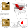 |
Fig. 2. Illustration of how a bright patch group is defined. a: 1−8 min bandpass-filtered IRIS SJI 2796 Å image. b: Gaussian filtered SJI image. c: binary map. The red area indicates the extracted umbral flash. d: 3D binary map. The red volume indicates an umbral flash event. |
We produced a 3D binary cube B(x, y, t) by stacking binary maps for each observing time. In the binary cube a group of connected voxels can be obtained (Fig. 2d). We defined the group of voxels as an umbral flash event, which is regarded as a phenomenon that occurs as a wavefront with the same propagation phase (Cho & Chae 2020). We only selected umbral flash events with a lifetime longer than 65 s (identified in five successive images). The effective size of the umbral flash events was defined as the mean value of the effective size of the umbral flashes composing that event. The time cadence of the IRIS SJIs is short enough to follow individual umbral flash events. In our data the typical size and horizontal speed of the umbral flashes are approximately 2000 km and 40 km s−1, respectively (see Figs. 4 and 7b), which is consistent with previous reports (e.g., Beckers & Schröter 1969). It implies that an umbral flash generally takes about 50 s to move away from its original position, which is much longer than the IRIS SJI time cadence of 13 s. There might be a concern that extremely fast-moving umbral flashes (2000 km/13 s ≳ 150 km s−1) could be identified as separate umbral flash events. However, such an event would be split into several events with shorter lifetimes, so it is very likely for them to be filtered out by our lower limit of lifetime (65 s).
The center of each umbral flash UFcen was determined by the 2796 Å intensity-weighted center
 (1)
(1)
The position of an UFcen is located inside that umbral flash except in some special cases when the umbral flashes are in the shape of an arc or concentric circle. These kinds of cases are rare, however, so we think the resulting error is statistically insignificant. We analyzed the motion of umbral flashes using the identified centers UFcen. The center of the first detected umbral flash, which is the bottom-most part in the 3D voxels, was determined as the oscillation center of the umbral flash event. This method is similar to that of previous studies using umbral flashes (Liang et al. 2011; Yurchyshyn et al. 2020) and umbral velocity oscillations (Cho et al. 2019). In these studies their origins were manually identified as the first detected positions of the umbral flashes or umbral oscillations. Figure 3 shows some examples of umbral flash events detected by our method. The merging or splitting of umbral flash events was frequently detected. We counted the umbral flash events based on the oscillation centers. We expect that the merging of different events may cause a small error in tracking their positions.
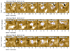 |
Fig. 3. Some examples of the identified umbral flash events. The background image is IRIS SJI 2796 Å and the umbral flashes identified by our method are indicated with blue contours. Each row shows the evolution of the identified umbral flashes for different events. The blue cross indicates the oscillation center. |
4. Results
Figure 4 and an animation associated with Fig. A.1 show the evolution process of the merging sunspot. It is very likely that there were two separate magnetic field structures at the initial stage. The two primordial sunspots were divided by a strong light bridge (Fig. 4a). The strong light bridge had a width of about 7″; it appears as a narrow photospheric region similar to the region outside of the sunspots. The light bridge became thinner and weaker with time, then eventually it disappeared (Fig. 4b). Finally, the two sunspots merged and became a single round sunspot. This process occurred within three days. The three SJI data sets we found show three stages of the light bridge: thin, faint, and extinct. The light bridge dividing the two sunspots existed near x = 0″ on Dec. 16, so we assumed an imaginary line with x = 0″ as the convergent interface.
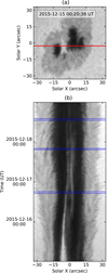 |
Fig. 4. Sunspot evolution observed by SDO/HMI intensitygram. a: initial stage of the merging sunspot on Dec. 15, 2015. The red solid line indicates the slit position for the following time-distance map. b: time-distance map of intensity from Dec. 15 to 18, 2015. The three time domains (blue solid lines) indicate the time covered by IRIS SJI data sets. |
We identified about 1000 umbral flashes for each of the SJI 2796 Å data sets. Only some of them satisfied our criteria described in the previous section and were counted as umbral flash events. The total number of selected umbral flash events increased from 78 to 99 and 135 for the three data sets.
Figure 5 shows the distributions of two parameters, the effective size and lifetime, of the selected umbral flash events. The effective size shows a normal distribution with a mean value of about 2.7″ and a standard deviation of about 0.2″. These values did not change significantly over time. Shorter lifetime events were found to be dominant. Most of the umbral flash events had a lifetime shorter than 150 s. The proportion of long-lasting events slightly increased with time. The effective size and the lifetime had a weak positive correlation. Long-lasting umbral flash events consisted of larger umbral flashes. It is not clear whether this tendency reflects the nature of the umbral flash events or if it is caused by the limitation of the algorithm related to the merging of the umbral flash events.
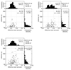 |
Fig. 5. Scatter plots between the effective size and lifetime of identified brightening features from the three SJI 2796 Å data sets. The probability density histogram of effective size and lifetime are shown respectively at the top and to the right of the scatter plots. The date, time, total number of the identified umbral flash events N, mean value m, and standard deviation σ are indicated in each panel. The dotted gray line indicates the mean value of each parameter. The methodological lower limits of the effective size and lifetime are 2″ and 65 s, respectively. |
Figures 6a and b show the detailed structure of the sunspot. On the first day the light bridge was split into two strands near the convergent interface. The two strands were deformed, weakened, and slightly closer to each other on the second day, and finally disappeared on the third day. The light bridge had weak magnetic field strength that was about 1000 G weaker than that of the umbral core which is consistent with previous reports (Beckers & Schröter 1969; Rueedi et al. 1995; Jurčák et al. 2006).
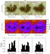 |
Fig. 6. Analysis results of spatial distribution of the identified oscillation centers. a: positions of the oscillation centers (red dots). The background image is from the IRIS SJI 2832 Å data, which shows the solar atmosphere at the photospheric height. The white ellipse and dashed line indicate a defined umbral region for identifying the umbral flashes and the convergent interface, respectively. b: HMI magnetic field strength map. The black contour indicates the umbral-penumbral boundary obtained from the IRIS SJI 2832 Å image. c: distribution of the oscillation centers from the convergent interface. Each column represents a different observation date. |
Figure 6a shows the spatial distribution of the oscillation centers for each data set. The most important finding is that the oscillation centers appear without any noticeable spatial relationship to the convergent interface. They are not crowded near the convergent interface indicated by the vertical dashed line in Fig. 6a. Figure 6c also clearly shows that the convergent interface (x = 0″) is not a special region for the oscillation centers. This characteristic persists in all three data sets.
A careful examination reveals some details on the spatial distribution of the oscillations. We find that there are voids, areas where there are very few oscillation centers or none at all. These voids may be partly attributed to the difficulty of identifying umbral flashes. The most representative example of such a void is the area around (−4″, 0″) on the first day (see Fig. 6a). There was a conspicuous light bridge in the photosphere of this area, and we found just a few oscillation centers within a radius of about 3″, which is matched by the abscissa value x = −4″ in Fig. 6c, first panel. We identified recursive strong jets anchored in this light bridge from the IRIS SJI 2796 Å data. This kind of jet occurrence may have kept us from clearly identifying the umbral flashes. Another example is found on the third day. In the right column of Fig. 6c a dip at x = 7″ can be seen because the IRIS slit, shown as a dark vertical line in the right column of Fig. 6a, had a fixed position as the observations were taken in sit-and-stare mode on the third day. Thus, the umbral flashes were not properly identified there on the third day.
We found that the voids occur as a result of the identification problem of umbral flashes, but it seems that some voids located on bright photospheric regions, such as light bridges and umbral dots, are real. In Fig. 6a it can be seen that the oscillation centers are not found at the core of the bright umbral dots or the light bridges, but several oscillation centers are located at their edges. Figure 6c shows this more clearly. In the histograms, dips are found at x = 4″ on the first day and x = 0″ on the second day. It indicates that fewer oscillation centers are found in the locations where bright umbral dots and light bridges were concentrated. We could not find strong jet phenomena there.
We investigated the characteristics of the IRIS SJI 2832 Å intensity and magnetic field strength in the HMI data at the oscillation centers (Fig. 7). The black scatter plot shows the relation between the two parameters at the oscillation centers. We also plotted the results from the IRIS SJI pixels composing the umbra in light blue. Both scatter plots clearly exhibit a negative correlation. However, there are differences between the photospheric characteristics at the positions of the oscillation centers and those in the whole umbra. The oscillation centers tend to occur in darker photospheric regions and stronger magnetic field locations known as dark nuclei of the umbral core (Sobotka et al. 1993). This is more clearly seen in each histogram. The probability density function of the photospheric intensity at the oscillation centers is similar to those from the whole umbra, but slightly more inclined toward lower intensity. The mean values of the IRIS SJI 2832 Å intensities at the oscillation center positions range from 11 DN to 14 DN, which are about 0.5σ lower than those from the whole umbra. Similarly, the oscillation centers are located above regions with a stronger magnetic field strength. The mean values of magnetic field strength at the oscillation centers range from about 2500 G to 2600 G, which is about 0.5σ higher than those of the whole umbra in each data set. These results agree with our finding in the above that the oscillation centers are not found near the light bridge and umbral dots (see Fig. 6).
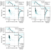 |
Fig. 7. Scatter plots between the IRIS SJI 2832 Å intensity and the HMI magnetic field strength. The format is similar to Fig. 5. The IRIS SJI 2832 Å intensity and magnetic field strength histograms are shown above and to the right, respectively, of each scatter plot. The black and light blue plots indicate respectively the results from the oscillation centers and the whole umbra defined by the inside of the ellipse in Fig. 6a. The IRIS SJI 2832 Å intensity is plotted in a logarithmic scale. |
We also analyzed the motions of the umbral flashes (Fig. 8a). The behavior of each umbral flash is quite complex, displaying azimuthal or rotating motion as well, which is consistent with previous reports (Rouppe van der Voort et al. 2003; Sych & Nakariakov 2014; Su et al. 2016; Felipe et al. 2019; Kang et al. 2019). Their behavior is quite distinct from the systematic photospheric motions of umbral dots and penumbral grains that move radially toward the center of the umbra (Sobotka & Puschmann 2009; Kilcik et al. 2020).
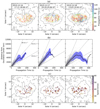 |
Fig. 8. Analysis results of the motion of umbral flashes. a: trajectory of the identified umbral flashes. The solid line indicates the movement of the center of the umbral flashes for each event. The color indicates the propagation time from the beginning of each event. b: time-distance plot of umbral flash motion. Each gray solid line represents the propagation of an umbral flash from its oscillation center. The black solid line and blue area indicate the mean value of the distance and standard deviation of the distance. The guidelines at 20, 40, and 80 km s−1 are shown with dashed lines. c: positions of the oscillation centers with averaged receding speed. The color corresponds to the averaged radial propagation speed, which is equivalent to the mean gradient of each gray line in (b). The black contour indicates the umbral-penumbral boundary in the IRIS SJI 2832 Å. Each column represents a different observational date. |
We find that umbral flashes recede from their oscillation centers. Figure 8b clearly shows that the distance between an umbral flash and its oscillation center increased with time in most cases. The receding speed ranges from 20 km s−1 to 80 km s−1 with a mean value of about 40 km s−1. This mean value persisted for about 150 s, and after that it started to decrease. We speculate that this decrease in the receding speed is presumably an error caused by the merging of long-lasting umbral flashes. Our results on the receding motion of umbral flashes are similar to the results on the apparent horizontal propagation of umbral oscillations previously reported by Cho et al. (2019), Kang et al. (2019), and modeled by Cho & Chae (2020).
We are able to estimate the source depth of the waves from the trajectory of the umbral flashes. Cho & Chae (2020) described the radial propagation of simple concentric umbral oscillations as an apparent motion. They modeled quasi-spherically propagating fast MHD waves below the photosphere and showed that the time lag near the photospheric level causes the apparent motion. According to their model, the radially receding speed from the oscillation center should be closely related to the source depth. A faster radially receding speed corresponds to a deeper source depth, which was also demonstrated by Felipe & Khomenko (2017) using numerical simulations. This relation is not only limited to a simple concentric propagation. Kang et al. (2019) presented an analytic solution of spiral wave patterns which appear as rotating umbral oscillations patterns with very complicated shapes. They showed that the radial and azimuthal motions are caused by fast MHD waves originating from a 1600 km source depth and cylindrical harmonic oscillations, respectively. Therefore, we believe that the radially receding speed shown in Figs. 8b and c is also closely related to the source depth although the model in Cho & Chae (2020) is simple, and the trajectories of the umbral flashes found here were chaotic (Fig. 8a).
Based on this interpretation, our results imply that the depth of the wave sources also seems not to be associated with the convergent interface. Cho & Chae (2020) showed that an average receding speed of 20 km s−1 to 40 km s−1 indicates about a 2000 km to 5000 km source depth. Simply applying this relation to our results, the light and dark dots in Fig. 8c indicate shallower (∼2000 km) and deeper (≥5000 km) depths, respectively. We can therefore conclude that shallow and deep sources were mixed inside the umbra, and there was no regional dependency of the source depth.
5. Discussion
In this study we investigated the subsurface structure of a merging sunspot by analyzing umbral flashes extracted from IRIS SJI Mg II 2796 Å images. We developed an algorithm to identify the umbral flashes and umbral flash events. Most of the umbral flash events had a lifetime shorter than 150 s and an effective size of about 2.7″. By tracking the motion of the umbral flashes we were able to determine the position of the oscillation centers. They are distributed over the whole umbra regardless of the convergent interface. They preferentially exist at the dark nuclei and tend to avoid the regions such as light bridges and umbral dots. We also estimated the source depth of the waves. According to our analysis, the source depths also showed no clear spatial dependence. These characteristics related to the umbral flashes changed little during the three merging stages.
Our finding of the distribution of the oscillation centers is consistent with previous reports. Liang et al. (2011) determined the positions of wave sources in Ca II H intensity image series, which is similar to oscillation centers. The 19 sources identified were found near the umbral cores away from the light bridge. Su et al. (2016) studied the interference of umbral waves on light bridges. They found that the umbral waves do not propagate from the light bridge, but move toward the light bridges. This also implies that oscillation centers do not exist near the light bridges. Yurchyshyn et al. (2020) reported that the origin of umbral flashes is mainly found in dark nuclei with a magnetic field strength of about 3000 G. Rouppe van der Voort et al. (2003) and Sych et al. (2020) also found that sources of chromospheric waves are displaced relative to the photospheric umbral dots. In line with these studies, we obtained the results that the oscillation centers are mainly located at the dark nuclei rather than near bright and weak field regions.
Our results support the notion that the subsurface structure of the sunspot is close to the cluster model. The oscillation centers are spread over the whole umbra. It implies that convection cells as the wave sources also exist everywhere beneath the photosphere. We emphasize that what we investigated is not a typical single sunspot, but a merging sunspot. Even though the merging sunspot consisted of two distinct environments represented by umbral cores and a convergent interface, it seems that this kind of special configuration does not affect the position of the convection cells. It signifies that the convergent interface of the merging sunspot may not differ from the umbral cores in the aspect of the wave generation. In other words, the field-free gaps that are supposed to exist below the convergent interface are likely to exist even below the subregions in the umbral cores. This finding closely matches the cluster model.
The distribution of the source depth also supports the cluster model. There was no regional dependency on the source depth. It indicates that the environment of the wave generation was not much different between the convergent interface and the umbral core. Moreover, all the characteristics from analyzing the umbral flashes persisted for the three days. This may imply that the subsurface structure of the sunspot did not change dramatically during the merging process because the sunspot was already an aggregation of small flux tubes. Therefore, we conjecture that the subsurface structure of the sunspot was similar to the cluster model.
Interestingly, our results are contrary to our previous studies from velocity oscillations. Chae et al. (2017) found strong oscillation power near a light bridge and umbral dot groups. Similarly, Cho et al. (2019) reported that individual umbral oscillation patterns originate from umbral dots. These findings of our previous studies are incompatible with our current results. This discrepancy may be partially resolved by noting that both previous studies used velocity oscillations inferred from the Fe I 5435 Å line formed around the temperature minimum region. There are two aspects to consider. One is the position error of oscillation centers caused by the propagating direction of waves from the low atmospheric level to the higher level. The other is the efficiency of nonlinearly developing strong intensity fluctuations from waves.
First, we note that the horizontal locations of oscillation centers may change with height if waves cannot propagate predominantly in the vertical direction. It is reported that the magnetic field configuration over light bridges is found to be complex (Felipe et al. 2016; Yuan & Walsh 2016; Toriumi et al. 2015). Similarly, umbral dots have a higher magnetic field inclination than other umbral regions (Socas-Navarro et al. 2004; Watanabe et al. 2009). Accordingly, as slow MHD waves propagate along the non-vertical magnetic field, the oscillation center determined at the upper atmosphere may deviate from the horizontal position of the wave source in a light bridge or an umbral dot.
Second, we note that umbral flashes preferentially occur in strong magnetic field environments. The intensity oscillations such as umbral flashes are considered to be a result of highly compressed gas by nonlinear propagation of slow MHD waves. It is likely that the gas compression may not fully develop in relatively weak field regions because the waveguiding effect of magnetic field is expected to be weaker in weaker field regions than in stronger field regions. This will cause a lower occurrence rate of umbral flashes in weak field medium. Light bridges are relatively weak field regions at the photosphere (Beckers & Schröter 1969; Rueedi et al. 1995; Jurčák et al. 2006). If this weak field environment extends to the upper atmosphere, fewer umbral flashes will be found above the light bridges. Umbral dots are also not free from this effect because of their weak field nature (Socas-Navarro et al. 2004; Riethmüller et al. 2008). Therefore, the configuration and strength of the magnetic field may cause a biased detection of wave phenomena.
To fully resolve the above discrepancy, further research based on velocity oscillations in the lower atmosphere is required. The velocity is more useful than intensity for the description of waves in a medium. Measurements at lower heights reduce the error of the oscillation center position arose from the magnetic field inclination. Therefore, we need to identify the relation between velocity oscillations at lower atmosphere and chromospheric umbral flashes and to draw a more solid conclusion on the subsurface structure of sunspots using it.
Movie
Movie associated with Fig. A.1. Access Supplementary Material
Acknowledgments
We greatly appreciate the referee’s constructive comments. This research was supported by Basic Science Research Program through the National Research Foundation of Korea (NRF) funded by the Ministry of Education (NRF-2020R1I1A1A01068789). MM acknowledges DFG-grant WI 3211/8-1. MM was supported by the National Research Foundation of Korea (NRF-2019H1D3A2A01099143, NRF-2020R1A2C2004616). IRIS is a NASA small explorer mission developed and operated by LMSAL with mission operations executed at NASA Ames Research Center and major contributions to downlink communications funded by ESA and the Norwegian Space Centre.
References
- Balthasar, H. 1999, Sol. Phys., 187, 389 [NASA ADS] [CrossRef] [Google Scholar]
- Beckers, J. M., & Schröter, E. H. 1969, Sol. Phys., 10, 384 [Google Scholar]
- Beckers, J. M., & Tallant, P. E. 1969, Sol. Phys., 7, 351 [NASA ADS] [CrossRef] [Google Scholar]
- Borrero, J. M., & Ichimoto, K. 2011, Liv. Rev. Sol. Phys., 8, 4 [Google Scholar]
- Centeno, R., Collados, M., & Trujillo Bueno, J. 2006, ApJ, 640, 1153 [Google Scholar]
- Chae, J., Lee, J., Cho, K., et al. 2017, ApJ, 836, 18 [Google Scholar]
- Cho, K., & Chae, J. 2020, ApJ, 892, L31 [NASA ADS] [CrossRef] [Google Scholar]
- Cho, K., Chae, J., Lim, E.-K., et al. 2019, ApJ, 879, 67 [NASA ADS] [CrossRef] [Google Scholar]
- Choudhuri, A. R. 1986, ApJ, 302, 809 [NASA ADS] [CrossRef] [Google Scholar]
- De Pontieu, B., Title, A. M., Lemen, J. R., et al. 2014, Sol. Phys., 289, 2733 [Google Scholar]
- Felipe, T., & Khomenko, E. 2017, A&A, 599, L2 [NASA ADS] [CrossRef] [EDP Sciences] [Google Scholar]
- Felipe, T., Collados, M., Khomenko, E., et al. 2016, A&A, 596, A59 [NASA ADS] [CrossRef] [EDP Sciences] [Google Scholar]
- Felipe, T., Kuckein, C., Khomenko, E., et al. 2019, A&A, 621, A43 [NASA ADS] [CrossRef] [EDP Sciences] [Google Scholar]
- Giovanelli, R. G. 1972, Sol. Phys., 27, 71 [NASA ADS] [CrossRef] [Google Scholar]
- Gizon, L., Schunker, H., Baldner, C. S., et al. 2009, Space Sci. Rev., 144, 249 [Google Scholar]
- Hoyle, F. 1949, Some Recent Researches in Solar Physics (Cambridge: Cambridge University Press) [Google Scholar]
- Jurčák, J., Martínez Pillet, V., & Sobotka, M. 2006, A&A, 453, 1079 [NASA ADS] [CrossRef] [EDP Sciences] [Google Scholar]
- Kang, J., Chae, J., Nakariakov, V. M., et al. 2019, ApJ, 877, L9 [NASA ADS] [CrossRef] [Google Scholar]
- Kilcik, A., Sarp, V., Yurchyshyn, V., et al. 2020, Sol. Phys., 295, 58 [NASA ADS] [CrossRef] [Google Scholar]
- Lee, J. W. 1993, ApJ, 404, 372 [NASA ADS] [CrossRef] [Google Scholar]
- Liang, H., Ma, L., Yang, R., et al. 2011, PASJ, 63, 575 [NASA ADS] [CrossRef] [Google Scholar]
- Lites, B. W. 1984, ApJ, 277, 874 [NASA ADS] [CrossRef] [Google Scholar]
- Meyer, F., Schmidt, H. U., Weiss, N. O., et al. 1974, MNRAS, 169, 35 [NASA ADS] [CrossRef] [Google Scholar]
- Moore, R. L. 1973, Sol. Phys., 30, 403 [NASA ADS] [CrossRef] [Google Scholar]
- Ortiz, A., Bellot Rubio, L. R., & Rouppe van der Voort, L. 2010, ApJ, 713, 1282 [Google Scholar]
- Parker, E. N. 1975, Sol. Phys., 40, 291 [NASA ADS] [CrossRef] [Google Scholar]
- Parker, E. N. 1979, ApJ, 234, 333 [NASA ADS] [CrossRef] [Google Scholar]
- Rempel, M. 2011, ApJ, 740, 15 [NASA ADS] [CrossRef] [Google Scholar]
- Riethmüller, T. L., Solanki, S. K., & Lagg, A. 2008, ApJ, 678, L157 [Google Scholar]
- Rouppe van der Voort, L. H. M., Rutten, R. J., Sütterlin, P., et al. 2003, A&A, 403, 277 [NASA ADS] [CrossRef] [EDP Sciences] [Google Scholar]
- Rueedi, I., Solanki, S. K., & Livingston, W. 1995, A&A, 302, 543 [NASA ADS] [Google Scholar]
- Rueedi, I., Solanki, S. K., Stenflo, J. O., et al. 1998, A&A, 335, L97 [Google Scholar]
- Schou, J., Scherrer, P. H., Bush, R. I., et al. 2012, Sol. Phys., 275, 229 [Google Scholar]
- Schüssler, M., & Vögler, A. 2006, ApJ, 641, L73 [Google Scholar]
- Sobotka, M., & Puschmann, K. G. 2009, A&A, 504, 575 [NASA ADS] [CrossRef] [EDP Sciences] [Google Scholar]
- Sobotka, M., Bonet, J. A., & Vazquez, M. 1993, ApJ, 415, 832 [NASA ADS] [CrossRef] [Google Scholar]
- Socas-Navarro, H., Martínez Pillet, V., Sobotka, M., et al. 2004, ApJ, 614, 448 [CrossRef] [Google Scholar]
- Su, J. T., Ji, K. F., Cao, W., et al. 2016, ApJ, 817, 117 [NASA ADS] [CrossRef] [Google Scholar]
- Sych, R., & Nakariakov, V. M. 2014, A&A, 569, A72 [NASA ADS] [CrossRef] [EDP Sciences] [Google Scholar]
- Sych, R., Zhugzhda, Y., & Yan, X. 2020, ApJ, 888, 84 [Google Scholar]
- Thomas, J. H., & Weiss, N. O. 2004, ARA&A, 42, 517 [Google Scholar]
- Tian, H., DeLuca, E., Reeves, K. K., et al. 2014, ApJ, 786, 137 [NASA ADS] [CrossRef] [Google Scholar]
- Toriumi, S., Cheung, M. C. M., & Katsukawa, Y. 2015, ApJ, 811, 138 [Google Scholar]
- Watanabe, H., Kitai, R., & Ichimoto, K. 2009, ApJ, 702, 1048 [NASA ADS] [CrossRef] [Google Scholar]
- Watanabe, H., Bellot Rubio, L. R., de la Cruz Rodríguez, J., et al. 2012, ApJ, 757, 49 [NASA ADS] [CrossRef] [Google Scholar]
- Yuan, D., & Walsh, R. W. 2016, A&A, 594, A101 [NASA ADS] [CrossRef] [EDP Sciences] [Google Scholar]
- Yurchyshyn, V., Kilcik, A., Şahin, S., et al. 2020, ApJ, 896, 150 [NASA ADS] [CrossRef] [Google Scholar]
- Zhao, J., Kosovichev, A. G., & Duvall, T. L. 2001, ApJ, 557, 384 [NASA ADS] [CrossRef] [Google Scholar]
- Zhao, J., Chen, R., Hartlep, T., et al. 2015, ApJ, 809, L15 [NASA ADS] [CrossRef] [Google Scholar]
Appendix A: Online material
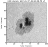 |
Fig. A.1. Animation sequence of the HMI intensitygram showing sunspot evolution for three days from 2015 Dec 15 00:20 UT. |
All Tables
All Figures
|
Fig. 1. Schematic representation of the hypothesis of this study. Left: cross sections of two merging sunspots in (a) the monolithic model and (c) the cluster model. The black solid arrows indicate magnetic field lines. The yellow region is a magnetic field-free region. The vertical dashed line indicates the convergent interface. The red circular arrows indicate the general convection cells. The opaque red circular arrows indicate the magneto-convection cells. Right: distributions of the oscillation centers on the plane of the sky (panels b and d). The oscillation centers are indicated with red concentric circles. |
| In the text | |
|
Fig. 2. Illustration of how a bright patch group is defined. a: 1−8 min bandpass-filtered IRIS SJI 2796 Å image. b: Gaussian filtered SJI image. c: binary map. The red area indicates the extracted umbral flash. d: 3D binary map. The red volume indicates an umbral flash event. |
| In the text | |
|
Fig. 3. Some examples of the identified umbral flash events. The background image is IRIS SJI 2796 Å and the umbral flashes identified by our method are indicated with blue contours. Each row shows the evolution of the identified umbral flashes for different events. The blue cross indicates the oscillation center. |
| In the text | |
|
Fig. 4. Sunspot evolution observed by SDO/HMI intensitygram. a: initial stage of the merging sunspot on Dec. 15, 2015. The red solid line indicates the slit position for the following time-distance map. b: time-distance map of intensity from Dec. 15 to 18, 2015. The three time domains (blue solid lines) indicate the time covered by IRIS SJI data sets. |
| In the text | |
|
Fig. 5. Scatter plots between the effective size and lifetime of identified brightening features from the three SJI 2796 Å data sets. The probability density histogram of effective size and lifetime are shown respectively at the top and to the right of the scatter plots. The date, time, total number of the identified umbral flash events N, mean value m, and standard deviation σ are indicated in each panel. The dotted gray line indicates the mean value of each parameter. The methodological lower limits of the effective size and lifetime are 2″ and 65 s, respectively. |
| In the text | |
|
Fig. 6. Analysis results of spatial distribution of the identified oscillation centers. a: positions of the oscillation centers (red dots). The background image is from the IRIS SJI 2832 Å data, which shows the solar atmosphere at the photospheric height. The white ellipse and dashed line indicate a defined umbral region for identifying the umbral flashes and the convergent interface, respectively. b: HMI magnetic field strength map. The black contour indicates the umbral-penumbral boundary obtained from the IRIS SJI 2832 Å image. c: distribution of the oscillation centers from the convergent interface. Each column represents a different observation date. |
| In the text | |
|
Fig. 7. Scatter plots between the IRIS SJI 2832 Å intensity and the HMI magnetic field strength. The format is similar to Fig. 5. The IRIS SJI 2832 Å intensity and magnetic field strength histograms are shown above and to the right, respectively, of each scatter plot. The black and light blue plots indicate respectively the results from the oscillation centers and the whole umbra defined by the inside of the ellipse in Fig. 6a. The IRIS SJI 2832 Å intensity is plotted in a logarithmic scale. |
| In the text | |
|
Fig. 8. Analysis results of the motion of umbral flashes. a: trajectory of the identified umbral flashes. The solid line indicates the movement of the center of the umbral flashes for each event. The color indicates the propagation time from the beginning of each event. b: time-distance plot of umbral flash motion. Each gray solid line represents the propagation of an umbral flash from its oscillation center. The black solid line and blue area indicate the mean value of the distance and standard deviation of the distance. The guidelines at 20, 40, and 80 km s−1 are shown with dashed lines. c: positions of the oscillation centers with averaged receding speed. The color corresponds to the averaged radial propagation speed, which is equivalent to the mean gradient of each gray line in (b). The black contour indicates the umbral-penumbral boundary in the IRIS SJI 2832 Å. Each column represents a different observational date. |
| In the text | |
|
Fig. A.1. Animation sequence of the HMI intensitygram showing sunspot evolution for three days from 2015 Dec 15 00:20 UT. |
| In the text | |
Current usage metrics show cumulative count of Article Views (full-text article views including HTML views, PDF and ePub downloads, according to the available data) and Abstracts Views on Vision4Press platform.
Data correspond to usage on the plateform after 2015. The current usage metrics is available 48-96 hours after online publication and is updated daily on week days.
Initial download of the metrics may take a while.