| Issue |
A&A
Volume 656, December 2021
|
|
|---|---|---|
| Article Number | A155 | |
| Number of page(s) | 15 | |
| Section | Galactic structure, stellar clusters and populations | |
| DOI | https://doi.org/10.1051/0004-6361/202141408 | |
| Published online | 16 December 2021 | |
Young giants of intermediate mass
Evidence of rotation and mixing⋆
1
GEPI, Observatoire de Paris, Université PSL, CNRS, 5 place Jules Janssen, 92195 Meudon, France
e-mail: This email address is being protected from spambots. You need JavaScript enabled to view it.
2
Department of Astronomy, University of Geneva, Chemin Pegasi 51, 1290 Versoix, Switzerland
3
IRAP, CNRS UMR 5277 and Université de Toulouse, 14 Avenue Edouard Belin, 31400 Toulouse, France
4
Departamento de Ciencias Fisicas, Universidad Andres Bello, Fernandez Concha 700, Las Condes, Santiago, Chile
5
INAF, Osservatorio Astronomico di Trieste, Via Tiepolo 11, 34143 Trieste, Italy
6
IFPU, Istitute for the Fundamental Physics of the Universe, Via Beirut, 2, 34151 Grignano, Trieste, Italy
7
INFN, Sezione di Trieste, Via A. Valerio 2, 34127 Trieste, Italy
8
Dipartimento di Fisica e Astronomia, Università degli Studi di Bologna, Via Gobetti 93/2, 40129 Bologna, Italy
9
INAF – Osservatorio di Astrofisica e Scienza dello Spazio di Bologna, Via Gobetti 93/3, 40129 Bologna, Italy
Received:
28
May
2021
Accepted:
24
September
2021
Abstract
Context. In the search of a sample of metal-poor bright giants using Strömgren photometry, we serendipitously found a sample of 26 young (ages younger than 1 Gyr) metal-rich giants, some of which have high rotational velocities.
Aims. We determined the chemical composition and rotational velocities of these stars in order to compare them with predictions from stellar evolution models. These stars where of spectral type A to B when on the main sequence, and we therefore wished to compare their abundance pattern to that of main-sequence A and B stars.
Methods. Stellar masses were derived by comparison of the position of the stars in the colour-magnitude diagram with theoretical evolutionary tracks. These masses, together with Gaia photometry and parallaxes, were used to derive the stellar parameters. We used spectrum synthesis and model atmospheres to determine chemical abundances for 16 elements (C, N, O, Mg, Al, Ca, Fe, Sr, Y, Ba, La, Ce, Pr, Nd, Sm, and Eu) and rotational velocities.
Results. The age-metallicity degeneracy can affect photometric metallicity calibrations. We identify 15 stars as likely binary stars. All stars are in prograde motion around the Galactic centre and belong to the thin-disc population. All but one of the sample stars present low [C/Fe] and high [N/Fe] ratios together with constant [(C+N+O)/Fe], suggesting that they have undergone CNO processing and first dredge-up. The observed rotational velocities are in line with theoretical predictions of the evolution of rotating stars.
Key words: stars: abundances / stars: evolution / stars: atmospheres
Based on observations obtained at Observatoire de Haute Provence, Canada-France-Hawaii Telescope and Telescopio Nazionale Galileo.
© L. Lombardo et al. 2021
 Open Access article, published by EDP Sciences, under the terms of the Creative Commons Attribution License (https://creativecommons.org/licenses/by/4.0), which permits unrestricted use, distribution, and reproduction in any medium, provided the original work is properly cited.
1. Introduction
The project Measuring at Intermediate metallicity Neutron Capture Elements (MINCE) (Cescutti et al., in prep.) has the goal of obtaining chemical abundances for stars in the intermediate metallicity range (− 2.5 ≤ [Fe/H] ≤ − 1). The aim is a detailed inventory of the neutron-capture elements.
The target selection of the first few observational runs in the northern hemisphere heavily relied on Strömgren photometry. As detailed in Sect. 2, this selection was unsuccessful in finding metal-poor giants. Its sample even proved to consist of young stars with masses in the range 2.5–6 solar masses in a narrow metallicity range of about solar metallicity.
The most frequently studied G-K stars in this mass range are particular cases of peculiar stars, such as Ba stars (Bidelman & Keenan 1951; Sneden et al. 1981; Antipova et al. 2003; Liang et al. 2003; Allen & Barbuy 2006; Smiljanic et al. 2007; Pereira et al. 2011; de Castro et al. 2016) and Cepheids (Lemasle et al. 2007, 2008, 2013; Genovali et al. 2014, 2015). As these stars were of A to B type when they were on the main sequence, the serendipitous discovery of this sample of giant stars allowed us to study this evolutionary stage directly. This stage is not very well characterised by observations so far because the time spent by stars in this phase is short. In addition, it allows a direct comparison with the properties of A- to B-type stars. For this reason, it is a unique opportunity for testing the predictions of stellar evolutionary models in terms of the evolution of chemical abundances and rotational velocities.
We expect a large number of such stars to be observed in the course of wide-field surveys such as WEAVE (Dalton et al. 2020) and 4MOST (de Jong et al. 2019). The findings of our investigation can be used to select these stars from the wide surveys.
2. Target selection
For the stars presented in this paper, we used the Strömgren photometry from the Paunzen (2015) catalogue and the metallicity calibration for giants of Casagrande et al. (2014) to select candidate intermediate-metallicity stars. To our surprise, all the stars appeared to be at about solar metallicity when we inspected the spectra, and several rotate rapidly (are therefore young and massive).
The question was whether a mistake was made in the star selection. We examined the synthetic photometry of Parsec solar metallicity isochrones of ages in the range 0.1–1 Gyr (Bressan et al. 2012). As shown in Fig. 1, in the region of the Gaia Early Data Release 3 (EDR3) (Gaia Collaboration 2016, 2021) colour-magnitude diagram in which our targets lie, the young solar metallicity isochrones clearly overlap the locus occupied by the red giant branch (RGB) of old metal-poor isochrones. This is what is meant by age-metallicity degeneracy. Furthermore, the Strömgren indices of many of the points along the young solar metallicity isochrones are within the validity range of the Casagrande et al. (2014) calibration. If they were used as input to the Casagrande et al. (2014) calibration, the majority of these photometric values would provide a metal-poor metallicity estimate. This is another manifestation of the age-metallicity degeneracy. The Casagrande et al. (2014) calibration in our opinion performs poorly on such metal-rich young stars because these stars were absent from the calibrators used by Casagrande et al. (2014) to define the calibration. However, even if these calibrators had been used, it is not clear if the degeneracy could have been lifted without introducing some age-sensitive quantity in the calibration.
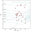 |
Fig. 1. Colour-magnitude diagram of Gaia EDR3 absolute magnitude G and dereddened colour GBP − GRP comparing the observed stars with Parsec isochrones with solar metallicity and ages between 0.1 and 1 Gyr (cyan), and with [Fe/H] = −2.0 dex and age 12 Gyr (grey). |
3. Observations
The spectra used in this paper have been obtained with three different telescopes and spectrographs. The log of the observations and the observed radial velocities are provided in Table 1.
Log of the observations.
3.1. SOPHIE at OHP
SOPHIE (Bouchy & Sophie Team 2006) is a fibre-fed high-resolution spectrograph operated at the Observatoire de Haute Provence (OHP) 1.93 m telescope. The spectra were obtained in visitor mode during three nights from September 13th to 16th 2019, the observer was one of the co-authors (A.d.M. Matas Pinto). The SOPHIE high-resolution mode, which provides a resolving power R ∼ 75 000, was used for all the observations. The spectral range we covered is 387.2 nm to 694.3 nm. The wavelength calibration relied on a Th-Ar lamp and on a Fabry-Pérot etalon. The data were reduced automatically on the fly by the SOPHIE pipeline. Radial velocities (vrad) were provided with the K5 template from the SOPHIE pipeline. For HD 192045 and HD 213036, the SOPHIE pipeline failed because the input radial velocity, taken from the Gaia second data release (hereafter Gaia DR2, Gaia Collaboration 2016, 2018; Arenou et al. 2018; Sartoretti et al. 2018), was too different from the observed radial velocity of the star. The vrad were derived by us by measuring the cross-correlation function over the interval 500 nm ≤ λ ≤ 650 nm. A synthetic template with appropriate stellar parameters was used.
3.2. ESPaDOnS at CFHT
ESPaDOnS (Donati et al. 2006) is a fibre-fed spectropolarimeter operated at the 3.6 m Canada-France-Hawaii telescope (CFHT) on the summit of Mauna Kea. The observation were obtained in the Queued Service Observation mode of the CFHT in November 2019. The spectroscopic mode “Star+Sky” was used, providing a resolving power of R ∼ 65 000. It covers the spectral range 370 nm–1051 nm. The data were delivered to us reduced with the Upena pipeline1, which uses the routines of the Libre-ESpRIT software (Donati et al. 1997). The output spectrum is provided in an order-by-order format. We merged the orders using an ESO-MIDAS2 script written by ourselves. Radial velocities were derived measuring the cross-correlation function over the interval 420 nm ≤ λ ≤ 680 nm.
3.3. HARPS-N at TNG
HARPS-N (Cosentino et al. 2012) is a fibre-fed high-resolution spectrograph operated at the 3.5 m Telescopio Nazionale Galileo (TNG) at the Canary Island La Palma. It is essentially a copy of HARPS (Mayor et al. 2003), operated by ESO on its 3.6 m telescope at La Silla. The observations were obtained in service mode in December 2019. We used the high-resolution mode, which provides a resolving power R ∼ 115 000. The wavelength range covered is 383 nm to 690 nm. The data were reduced on the fly by the HARPS pipeline. Radial velocities were provided with the G2 template from the HARPS-N pipeline.
4. Analysis
4.1. Stellar parameters
To derive stellar parameters, we used Gaia EDR3 photometry (G and GBP − GRP) and parallaxes. We defined a grid in the parameter space using the ATLAS 9 model atmosphere grids by Mucciarelli et al. (in prep.). The range of atmospheric parameters covered by the grid is shown in Table 2.
Range of atmospheric parameters of the ATLAS 9 model atmosphere grid.
We computed theoretical values of GBP − GRP, bolometric correction (BCG), and extinction coefficients AG, E(GBP − GRP) using the reddening law of Fitzpatrick et al. (2019) for the whole grid. Effective temperatures (Teff) and surface gravities (log g) were derived iteratively with the following procedure:
-
The mass and the metallicity of the star were fixed at input values.
-
Teff was derived by interpolating in GBP − GRP at fixed metallicity, and the bolometric correction was derived by interpolation from the new Teff.
-
log g was derived using Teff and bolometric correction found in the previous step from the equation
 (1)
(1)where M is the stellar mass, G0 is the dereddened apparent G magnitude, BCG is the bolometric correction, and p is the parallax.
-
AG and E(GBP − GRP) were derived by interpolating in the theoretical grid adopting the E(B − V) from STILISM maps (Capitanio et al. 2017).
-
G and GBP − GRP were dereddened using E(GBP − GRP).
-
The procedure was iterated until the difference between the new and the old Teff was smaller than ±50 K and the difference between the new and the old log g was smaller than 0.05 dex.
After we derived the stellar parameters, we used the measured equivalent widths (EWs) of the Fe I lines (see Sect. 4.2) and the GALA code (Mucciarelli et al. 2013) to derive the metallicity of the stars. With the new metallicity values, we again derived the stellar parameters and stopped the iteration when the difference between the new and the old Teff was smaller than ±50 K. To confirm the values of Teff and log g obtained from the procedure, we derived effective temperatures and surface gravities using a new implementation of the Mucciarelli & Bellazzini (2020) InfraRed Flux Method (IRFM) colour-Teff calibration for giants stars based on EDR3 data (Mucciarelli et al. 2021). The two effective temperatures agree well, in particular, Teff from IRFM calibration is 70 K cooler on average than those estimated with the method described above.
As final parameters, we adopted Teff and log g derived from the Mucciarelli et al. calibration because the IRFM method is less dependent on the adopted models with respect to the method described in the procedure. We fixed the uncertainty on Teff at ±100 K, according to the dispersion of the Mucciarelli et al. calibration. In Table 3 we present the stellar parameters. Microturbulent velocities (ξ) were estimated using the calibration derived by Dutra-Ferreira et al. (2016). The uncertainty on ξ is ±0.1 km s−1 according to the uncertainty of Dutra-Ferreira et al. calibration.
Coordinates, atmospheric parameters, metallicities, and rotational velocities of the observed stars.
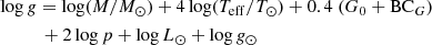
In Fig. 2 we compare Gaia EDR3 photometry of the observed stars to the Ekström et al. (2012) evolutionary tracks without rotation at solar metallicity for stellar masses between 2.5 M⊙ and 6.0 M⊙ provided by the SYCLIST code (Georgy et al. 2014), or interpolated between fully computed tracks. From Fig. 2 we deduce that these stars are very young, with ages between 0.1 Gyr (0.06 Gyr if we consider the evolutionary track for 6 M⊙) and 0.55 Gyr. The stellar masses we deduced from the evolutionary tracks are listed in Table 3. The uncertainty on stellar mass depends on the parallax error and on the stellar model adopted. If we adopt stellar models with rotation, for example, the evolutionary tracks are more luminous than the respective tracks without rotation (see Fig. 10 in Georgy et al. 2013). For this reason, we estimate an uncertainty in mass from 0.5 M⊙ for the less massive stars to 1 M⊙ for those that lie in the region of the colour-magnitude diagram in which different evolutionary tracks overlap. We estimated an uncertainty of ±0.1 dex on log g by varying the stellar mass in Eq. (1) according to the mass error.
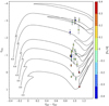 |
Fig. 2. Colour-magnitude diagram of Gaia EDR3 absolute magnitude G and dereddened colour GBP − GRP comparing the observed stars with Ekström et al. (2012) evolutionary tracks without rotation at metallicity Z = 0.014 for stellar masses between 2.5 M⊙ and 6.0 M⊙. Error bars represent the uncertainty on Gabs, corresponding to 3σ error on parallax. The colour index indicates our derived [Fe/H] of the stars. |
4.2. Iron abundances
Fe abundances were derived from the EW of the lines. The EWs were measured with the FITLINE code developed by P. François (Lemasle et al. 2007). FITLINE is a semi-interactive FORTRAN program that measures EWs of high-resolution spectra using genetic algorithms (Charbonneau 1995). Lines are fitted by a Gaussian defined by four parameters: the central wavelength, the width and depth of the line, and the continuum value. For each line, the algorithm runs as follows: (1) the program generates an initial set of Gaussians, giving random values to the four parameters of the Gaussian. (2) The fit quality is estimated by calculating the χ2. (3) A new “generation” of Gaussians is calculated from the 20 best fits after adding random modifications to the initial set of parameters. (4) The new set of parameters replaces the old set, and its accuracy is estimated again using a χ2 evaluation. Finally, (5) the process is iterated until the convergence to the best Gaussian fit is achieved. For the most highly rotating stars (HD 21269, HD 278, HD 40509, HD 55077, and HD 61107) FITLINE was modified to take the Gaussian and rotational profile of the lines into account. To derive Fe abundances from EWs, we used the GALA code (Mucciarelli et al. 2013), which compares the measured EW for each line with the theoretical EW computed from the curve of growth of the line. The Fe I and Fe II abundances we derived for this sample of stars are listed in Table 3.
4.3. Rotational velocities
Rotational velocities (v sin i) were measured by fitting the observed line profiles with the corresponding theoretical line profiles that were obtained from a synthetic spectrum computed with the spectral synthesis code SYNTHE (Kurucz 2005; Sbordone et al. 2004) based on ATLAS 9 1D plane-parallel model atmospheres (Kurucz 2005). In order to better compare v sin i between different stars, we selected a set of Fe I lines to be fitted. The list of Fe I lines we used to measure v sin i is shown in Table 4. For each line, we performed a χ2 minimisation fit on the observed line profile using three synthetic spectra computed with different rotational velocities. The metallicity of the synthetic spectra was fixed at the value of iron abundance derived from the EW of the single line. We made the assumption that the line broadening of synthetic spectra was equal to the instrumental broadening. The values of v sin i we obtained are presented in Table 3. This approach does not allow us to distinguish between v sin i and other sources of line broadening, such as macroturbulence. The spectra of five stars with similar Teff but different v sin i are shown in Fig. 3. For the faster-rotating stars, the line profile is dominated by the rotational profile, and we can assume that other broadening effects are negligible with respect to v sin i. For the more slowly rotating stars, however, the contribution of macroturbulence in line broadening is comparable to the rotational contribution, so that the values of v sin i obtained for these stars must be interpreted as upper limits.
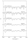 |
Fig. 3. Spectra of five stars with similar Teff and different v sin i. The spectra have been normalised and are shifted to facilitate visualisation. |
Fe I lines used to derive the rotational velocity of stars.
4.4. Chemical abundances of other elements
We were able to derive for the stars in the sample the elemental abundances of C, N, O, Mg, Al, and Ca and for the neutron capture elements Sr, Y, Ba, La, Ce, Pr, Nd, Sm, and Eu. For all elements we adopted the solar abundances determined by Caffau et al. (2011) and Lodders et al. (2009) (see Table 5). The chemical abundances we obtained are listed in Tables A.1–A.3. The values A(X) are expressed in the form A(X) = log(X/H) + 12. The abundance ratios [X/Fe]3 are expressed as [X/Fe]=[X/H]−[Fe/H] for elements up to Ca and as [X/Fe]=[X/H]−[FeII/H] for O and n-capture elements.
Solar abundance values adopted in this work.
The carbon abundance was derived from the G-band by minimisation of the χ2 when we compared the observed spectrum to a grid of synthetic spectra with different C abundances. The synthetic spectra were computed with SYNTHE (Kurucz 2005) using the ATLAS 9 model (Kurucz 2005) computed for each star (see Bonifacio & Caffau 2003, for details). The G-band is strong for all the stars, and we estimate an uncertainty in the range 0.2–0.5 dex in the C abundances, which is mainly related to the continuum placement. The nitrogen abundances were determined in a similar way using the violet CN band at 412.5 nm, assuming the C abundance derived from the G-band to be fixed. The error is mainly due to the uncertainty of placing the continuum and is in the range 0.3–0.6 dex. Oxygen was determined from the EW of the [OI] 630 nm line. This was measured with the iraf4 task splot only when the line was not affected by blends with telluric lines or the blend was minor and could be taken into account using the deblend option of splot. Mg, Al, and Ca abundances were derived using the procedure described in Sect. 4.2. The uncertainty showed in Table A.2 represents the line-to-line scatter if the abundance was derived from ≥2 lines, otherwise it represents the abundance error due to continuum placement. For the neutron-capture elements, the abundance was determined by matching the observed spectrum around each line of the list with a synthetic spectrum computed using the local thermodynamic equilibrium (LTE) spectral line analysis code turbospectrum (Alvarez & Plez 1998; Plez 2012), which treats scattering in detail. The computed errors in the elemental abundances ratios due to uncertainties in the stellar parameters are listed in Table A.4. The errors were estimated varying Teff by ±100 K, log g by ±0.5 dex, and ξ by ±0.5 dex in the model atmosphere of HD 13882. The results for other stars are similar. The main uncertainty comes from the error in the continuum placement when the synthetic line profiles are matched to the observed spectra. This error is of the order of 0.1 dex. When several lines are available, the typical line-to-line scatter for a given element is 0.1 dex.
5. Possible binary stars
Stars HD 195375 and HD 278 are listed in the Washington Double Star Catalog (Mason et al. 2001). We checked the Gaia EDR3 astrometric parameters of these two binary systems. We found that HD 278 and its companion have different parallaxes, so that these stars are probably in a visual double system but not in a physical one, as suggested by Muller (1984). In contrast, HD 195375 and its companion have consistent parallaxes, which implies that they are in a physical binary system. As binarity is a possible cause of radial velocity variability, we compared our measured radial velocities with those of Gaia DR2 (Gaia Collaboration 2018). The brightness of our stars implies that the error on the radial velocity due to photon noise is smaller than 1 km s−1 (Sartoretti et al. 2018). As shown in Table 6, six stars have a larger error, which means that they are very likely radial velocity variables. The Gaia radial velocity of eight stars differs by more than 5σ from our measured velocity. They are again very likely radial velocity variables. Ten stars have been identified as probable binary stars by Kervella et al. (2019) from the comparison between HIPPARCOS (ESA 1997) and Gaia DR2 proper motions. We note that stars HD 192045 and HD 213036 show all the properties mentioned above. This strongly suggests that they are binary stars. It is likely that the end-of-mission Gaia data, which will combine astrometry, epoch photometry, and radial velocities, will allow us to determine the orbits of the confirmed binaries.
Comparison between Gaia DR2 and observed radial velocities for our stars.
6. Kinematics and Galactic orbits
We characterised the stellar orbital parameters with the Galpot code5 (McMillan 2017; Dehnen & Binney 1998) using the stellar coordinates, radial velocities, Gaia DR2 distances, and proper motions. We derived the stellar coordinates and velocity components in the galactocentric cylindrical (R, z, φ, vR, vZ, vφ) and Cartesian systems (X, Y, Z, vX, vY, vZ). We derived the minimum and maximum cylindrical (Rmin, Rmax) and spherical (rmin, rmax) radii, the eccentricity (e = (rmax − rmin)/(rmax + rmin)), the maximum height above the Galactic plane (Zmax), the total energy (E), and the z-component of the angular momentum (LZ). We found that all stars have typical disc kinematics. All stars have prograde motions, and the eccentricity (e < 0.11) for 25 out of 26 stars (e ∼ 0.2 for HD 278) is very low. The maximum height above the Galactic plane is lower than 400 pc for 25 out of 26 stars (Zmax ∼ 600 pc for TYC 2813-1979-1).
7. Discussion
7.1. Photometric logg versus spectroscopic logg
In order to verify the values of log g that we obtained from Gaia photometry and parallaxes, we derived surface gravities by imposing the ionisation equilibrium of the Fe I and Fe II lines. As shown in Table 7, photometric and spectroscopic log g are compatible within 0.1 dex for ten stars, while the difference between photometric and spectroscopic gravities is −0.6 ≤ Δ log g ≤ 0.9 dex for the remaining stars. We deduced the corresponding stellar masses from spectroscopic gravities by inverting Eq. (1). We obtained that the masses should be 0.7 ≤ M/M⊙ ≤ 18.9; two stars have M < 0.8 M⊙. These very low masses are incompatible with stellar evolutionary models (unless we assume that they are older than 14 Gyr). We therefore conclude that the spectroscopic gravities are not reliable for the majority of these stars. The reason for the observed discrepancy is not trivial because for solar metallicity stars, we expect spectroscopic and photometric approaches to be equivalent (see the discussion in Mucciarelli & Bonifacio 2020). As the difference in log g reflects the difference between Fe I and Fe II abundances, the discrepancy for the most highly rotating stars could be due to a bias in the line selection. Stellar rotation allowed us to detect only the strongest and consequently most saturated Fe II lines. However, the same discrepancy is found for some stars with low rotational velocity, therefore some other effect must be responsible for it. The observed scatter in Δ log g for stars with v sin i < 10 km s−1 seems to suggest that this effect is due to inadequacies of the adopted physics, in particular, the assumption of 1D geometry and LTE, as discussed for metal-poor giants in Mucciarelli & Bonifacio (2020). We confirmed that non-LTE (NLTE) effects under the assumption of 1D geometry are not sufficient to solve the log g discrepancy. We applied the NLTE corrections provided by Bergemann et al. (2012)6 to the Fe I lines of the star HD 191066, for which we obtained [FeI/FeII] = 0.26 dex using photometric log g. We found that the mean correction value was 0.005 dex with a maximum value of 0.06 dex for the Fe I line at 5956.693 Å. This means that applying this NLTE correction to Fe I the imbalance would be even worse.
Comparison between photometric and spectroscopic log g and derived stellar masses.
7.2. Chemical composition
7.2.1. C, N, O
In Fig. 4 we show our measured C, N and O abundance ratios. The [C/Fe] ratios are lower than solar for all stars in our sample (⟨[C/Fe]⟩ = −0.44 dex and σ = 0.17), with the exception of two stars with [Fe/H] ∼ 0.4 dex that show a [C/Fe] of about zero. Our interpretation is that all the stars with sub-solar [C/Fe] show material in the photosphere that has been mixed with material that has experienced nuclear hydrogen burning through the CNO cycle. This interpretation is supported by the super-solar [N/Fe] ratios. The [(C+N+O)/Fe] ratio is shown in Fig. 5. This quantity is nearly constant and close to the solar value within the error bars. This indicates that the underabundances in C and the overabundances in N result from pure H-burning via the CNO cycle, and that no He-burning products have yet been transported to the stellar surface. The value of [C/Fe] of a given star is probably independent of the original [C/Fe] value that characterised the star on the main sequence, but depends only on the amount of mixing. This is supported by the fact that there is no clear trend of [C/Fe] with metallicity. If our interpretation is correct, the two more metal-rich stars of our sample are mixed very little with respect to the others. Some mixing is only suggested by a slight enhancement of [N/Fe] in both stars. These two stars belong to the stars with the highest gravity in the sample, which is in line with the notion of little or no mixing. We caution, however, that there are stars with similarly high log g that have a low [C/Fe]. There clearly is no one-to-one correspondence between surface gravity and mixing.
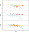 |
Fig. 4. [C/Fe], [N/Fe] and [O/Fe] abundances as a function of [Fe/H]. Comparison with targets from Takeda et al. (2018) (cyan crosses), Royer et al. (2014) (blue squares), Delgado Mena et al. (2010) (yellow crosses) and Ecuvillon et al. (2004) (grey diamonds). |
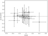 |
Fig. 5. [(C+N+O)/Fe] abundance ratios as a function of [Fe/H]. |
It is interesting to compare our results with those in the literature. We selected two samples of CNO abundances in A-type stars (Takeda et al. 2018 and Royer et al. 2014). The Takeda and Royer samples both consists of A-type main-sequence stars. Royer stars are also characterised by v sin i ≤ 65 km s−1. We also added samples of CNO samples in FGK dwarf stars with a metallicity comparable to that of our sample: Delgado Mena et al. (2010) provided C and O abundances for 370 FGK dwarfs stars, and Ecuvillon et al. (2004) provided N abundances for 91 solar-type stars. The top panel of Fig. 4 clearly shows that the majority of our stars have lower [C/Fe] than the FGK dwarfs (yellow crosses), with the exception of the two stars with the highest metallicity, which appear to be quite compatible. It is striking that the [C/Fe] abundance in A-type stars displays a decreasing trend with increasing metallicity for the samples of Takeda et al. (2018) (cyan crosses) and Royer et al. (2014) (blue squares). This trend is at odds with the flat trend shown by FGK stars. This trend in A stars has been noted and discussed by Takeda et al. (2018, see also references therein). A stars show the phenomenon of chemical peculiarities (CP stars), which gives rise to many sub-classes of CP stars (see Ghazaryan et al. 2018, and references therein). The most popular explanation of the chemical peculiarities for most classes of CP stars is diffusion (see e.g., Richer et al. 2000, and references therein), possibly in the presence of rotational mixing (Talon et al. 2006). As pointed out by Takeda et al. (2018), this anti-correlation of [C/Fe] with [Fe/H] can be understood if the mechanism causing the chemical peculiarities acts in opposite directions for CNO and Fe. We do not detect any chemical peculiarities, except for the CNO pattern expected from mixing on the RGB and Ba (see Sect. 7.2.3). This strongly suggests that these peculiarities, even if they were present when the star was on the main sequence, are erased as the star evolves to the RGB by the onset of convective mixing as the star cools and its atmosphere is no longer in radiative equilibrium, as was the case while the star was on the main sequence.
7.2.2. Mg, Al, and Ca
Figure 6 shows Mg, Al, and Ca abundance ratios as a function of [Fe/H]. Our results are compared to the analysis by Adibekyan et al. (2012) (yellow crosses) and Royer et al. (2014) (blue squares). The Adibekyan sample consists of F, G, and K dwarf stars, which means that they have lower masses than our sample stars, but Teff is similar. Our derived [Mg/Fe], [Al/Fe], and [Ca/Fe] abundance ratios appear to be in line with the results obtained by other authors. The dispersion in [Mg/Fe] (⟨[Mg/Fe]⟩ = 0.10 dex and σ = 0.16), [Al/Fe] (⟨[Al/Fe]⟩ = 0.02 dex and σ = 0.17) and [Ca/Fe] (⟨[Ca/Fe]⟩ = 0.06 dex and σ = 0.15) is larger than is expected from our estimated errors. In the case of [Mg/Fe], we note that the Adibekyan et al. and Royer et al. stars also show a large dispersion despite the high quality of spectra. The observed scatter is therefore probably intrinsic. The [Mg/Fe] ratio of two stars in our sample appears to be compatible with the values of stars in the upper sequence in the Adibekyan et al. sample. They were labelled thick-disc stars by the authors. However, the kinematics of these two stars clearly shows that they are thin-disc stars. A purely chemical selection is not sufficient to distinguish between thin- and thick-disc stars, as has been pointed out by several authors (see e.g., Franchini et al. 2020; Romano et al. 2021). Specifically, Romano et al. (2021) reported that only 25% of the high-α stars in their sample can be classified kinematically as belonging to the thick-disc population. It is therefore not surprising that we find thin-disc high-α stars. Some unexpected results were found for stars HD 278 and HD 21269. Star HD 278 shows a higher Al abundance than the other stars in the sample ([Al/Fe] = 0.55 dex, σ = 0.24). Star HD 21269 instead shows a higher than solar Mg abundance ([Mg/Fe] = 0.11 dex, σ = 0.36) and lower than solar Al and Ca abundance ([Al/Fe] = −0.30 dex, σ = 0.11; [Ca/Fe] = −0.47, σ = 0.26). These stars rotate rapidly (v sin i ∼ 22 km s−1 for HD 278 and v sin i ∼ 16 km s−1 for HD 21269) and the uncertainty on the abundances is large. As discussed in Sect. 7.1, rotation can affect the estimate of the EW of the lines, which may lead to an incorrect abundance estimate. However, we note that some stars in the Adibekyan et al. sample show the same Al abundance. This implies that it is possible for a star to have such a low [Al/Fe] ratio.
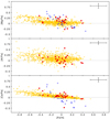 |
Fig. 6. [Mg/Fe], [Al/Fe], and [Ca/Fe] abundances as a function of [Fe/H]. Comparison with targets from Adibekyan et al. (2012) (yellow crosses) and Royer et al. (2014) (blue squares). |
7.2.3. Neutron-capture elements
In Figs. 7–9 we show the abundances of several neutron-capture elements. The Sr abundance ratio is compared to the analysis by Royer et al. (2014) (blue squares) and Battistini & Bensby (2016) (grey crosses), and the [Y/Fe] and [Ba/Fe] ratios are compared to the results of the analysis by Royer et al. (2014) (blue squares) and Bensby et al. (2014) (grey crosses). The La, Ce, Nd, Sm, and Eu abundances ratios are compared to the analysis by Battistini & Bensby (2016) (grey crosses). The Bensby et al. (2014) sample consists of F and G dwarf and subgiant stars, and Battistini & Bensby (2016) provided abundances of several n-capture elements for the same stars. We observe that in the case of n-capture elements, the abundances ratios we measured are also in line with the results found by other authors. A remarkable result is the Ba abundance, which is higher than solar for the majority of stars in our sample. The same result has been found for main-sequence stars by Royer et al. (2014). The NLTE correction for Ba lines provided by Korotin et al. (2015) would decrease the Ba abundances by 0.1 dex, which is insufficient to match the observed values with other n-capture abundances. We exclude the possibility that an atmospheric phenomenon could explain the observed Ba abundance: if the Ba overabundance were due to atmospheric processes during the main-sequence phase, it would be erased by mixing when the star evolves to the red giant phase.
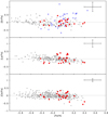 |
Fig. 7. [Sr/Fe], [La/Fe], and [Ce/Fe] abundances as a function of [Fe/H]. Comparison with targets from Battistini & Bensby (2016) (grey crosses) and Royer et al. (2014) (blue squares). |
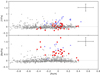 |
Fig. 8. [Y/Fe] and [Ba/Fe] abundances as a function of [Fe/H]. Comparison with targets from Bensby et al. (2014) (grey crosses) and Royer et al. (2014) (blue squares). |
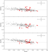 |
Fig. 9. [Nd/Fe], [Sm/Fe], and [Eu/Fe] abundances as a function of [Fe/H]. Comparison with targets from Battistini & Bensby (2016) (grey crosses). |
In Fig. 10 we compare our results to the s-process abundance ratios [s/Fe], that is, the mean abundance ratio [X/Fe] of s-process elements [Y/Fe], [La/Fe], [Ce/Fe], and [Nd/Fe] of barium stars derived by de Castro et al. (2016). We observe that three stars in our sample have [s/Fe] above 0.25 dex, which is the lower limit for [s/Fe] in Ba stars according to de Castro et al. (2016), and only one star (HD 63856) has [s/Fe] = 0.38 dex. These low values of the [s/Fe] ratio are compatible with those of mild Ba stars, which have weaker s-process enhancements than classical barium stars, only few or no anomalous molecular band strengths (Eggen 1972; Morgan & Keenan 1973), and no carbon enrichment (Sneden et al. 1981). However, we stress that the Ba II abundance is strongly dependent on microturbulent velocity. We note that an increase in microturbulence of 0.6 km s−1 decreases the Ba abundance by 0.6 dex for star HD 55077. This effect was first observed by Hyland & Mould (1974), who showed that high microturbulent velocities might cause the Ba II resonance lines to become anomalously strong in stars with solar s-process elements. In our case, we have no observation that supports such a high microturbulence, which would also affect the abundances of other elements. There probably is no strong evidence implying that stars in our sample are mild Ba stars, but the high [Ba/Fe] ratios are puzzling and unexplained.
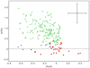 |
Fig. 10. Mean abundance ratio [s/Fe] of s-process elements ([Y/Fe], [La/Fe], [Ce/Fe], and [Nd/Fe]) as a function of [Fe/H]. Red circles represent the [s/Fe] ratio for the stars analysed in this work. Green squares represent barium stars analysed in de Castro et al. (2016). Black squares represent the targets rejected as barium stars in de Castro et al. (2016). |
In their study of dwarf stars in five open clusters and one star-forming region, Baratella et al. (2021) found an enhancement in Ba similar to what we have found in our stars. Remarkably, Ba is more enhanced for the younger clusters. The Ba enhancement is accompanied by mild Y enhancement of the order of 0.2 dex. A larger enhancement is again found for the younger clusters. These two results are consistent with our findings. At face value, our derived [Y/Fe] abundance ratios are ∼0.2 dex, but we do not give much weight to the Y enhancement as it is consistent with [Y/Fe] = 0 within the errors. Baratella et al. (2021) examined several causes for this Ba anomaly, including the role of magnetic fields. They failed to propose any convincing explanation of their observations, however. We therefore conclude that the increase in Ba that we observe may be related to what has been observed in other young stars.
7.2.4. Chemical abundances and rotational velocities
We investigated the presence of trends between elemental abundances and rotational velocity in our sample. To limit evolutionary effects, we considered only stars with metallicity in the range −0.1 < [Fe/H]< 0.1. We found that for only four elements ([O/H], [Ca/H], [Ba/H], and [Eu/H]) does non-parametric Kendall’s τ test provides a correlation probability higher than 95% with v sin i. However, parametric fitting did not confirm any trend between these quantities. We therefore conclude that the correlations are not significant.
7.3. Comparison with models
We compared our results with the predictions of two sets of stellar evolution models including the effects of rotation: the models of Georgy et al. (2013), which were computed with the Geneva stellar evolution code (GENEC), and the models of Lagarde et al. (2012), which were computed with the code STAREVOL (Mowlavi & Forestini 1994; Siess et al. 2000; Palacios et al. 2003, 2006; Decressin et al. 2009); see Lagarde et al. (2012) for a comparison between these two sets of models.
Because the observed rotational velocities depend on the inclination angle of the stars along the line of sight, a direct comparison between observed and predicted rotational velocities is not possible. However, the observed values of v sin i are lower limits for the actual surface rotation of stars. As shown in the upper panel of Fig. 11, the v sin i we obtained for stars with 3.5 M⊙ and 4 M⊙ in the metallicity range −0.1 < [Fe/H]< 0.1 (5 < v sin i < 22 km s−1) are compatible with the rotational velocity values predicted by the Georgy et al. models with 0.3 < ω < 0.67 at solar metallicity for stars in the corresponding region of the log Teff versus log g diagram.
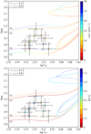 |
Fig. 11. Log Teff vs. log g diagram for the Georgy et al. (2013) evolutionary tracks with Z = 0.014, M = 3 M⊙, 4 M⊙, and ω = 0.3 (solid lines) and 0.6 (dashed lines). Stars in the sample with −0.1 < [Fe/H]< 0.1 and M = 3.5 M⊙, 4 M⊙ are shown with error bars. Upper panel: colour index indicates the equatorial velocity for evolutionary tracks and the observed v sin i for sample stars. Lower panel: colour index indicates the [N/C] abundance ratio. |
As described in Sect. 7.2.1, we found that almost all stars in the sample show lower than solar C abundances and higher than solar N abundances. This indicates that the stars have undergone mixing and that the products of the H-burning CNO cycle are visible on the stellar surface. In the lower panel of Fig. 11, the observed [N/C] abundance ratios of stars with 3.5 M⊙ and 4.0 M⊙ in the metallicity range −0.1 < [Fe/H]< 0.1 are compared with the values predicted by the Georgy et al. models for stars in the same region of the log Teff versus log g diagram. The stars are warmer than the maximum extent of the clump, or blue loop, where stars are located when they undergo central He-burning. However, because this phase is much longer than the crossing of the Hertzsprung gap, we consider it to be highly probable that all the stars are on the clump. We also note that the [N/C] abundance ratios for the majority of stars are consistent with the values predicted for clump stars in the Georgy et al. models. For all these quantities, a similar agreement is obtained with the models of Lagarde et al. (2012), as shown in Fig. 12.
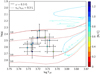 |
Fig. 12. Comparison between the Georgy et al. (2013) (solid lines) and Lagarde et al. (2012) (dashed lines) evolutionary tracks with rotation at Z = 0.014 for M = 3 M⊙, 4 M⊙. Stars in the sample with M = 3.5 M⊙, 4 M⊙ and −0.1 < [Fe/H]< 0.1 are shown with error bars. The colour index indicates the [N/C] abundance ratios. |
8. Conclusions
We observed a sample of 26 bright giant stars that had a photometric metallicity estimated to be in the range −2.5 ≤ [Fe/H]≤ − 1. The aim was a detailed inventory of the neutron-capture elements. The analysis of the sample showed that all stars were metal rich (−0.4 ≤ [Fe/H]≤0.4), with ages between 0.1 Gyr and 0.55 Gyr. Ten stars rotate rapidly (v sin i > 10 km s−1).
The main conclusions of our study are listed below.
-
Photometric metallicity calibrations may show an age-metallicity degeneracy.
-
Several stars show radial velocity variability, with an error on the Gaia DR2 radial velocity above 1 km s−1 and/or a Gaia DR2 radial velocity that differs by more than 5σ from our observed vrad. Ten stars have also been identified as binary stars by Kervella et al. (2019) from proper motion anomalies. Stars HD 192045 and HD 213036 show radial velocity and proper motion variations. We therefore suggest that they are binary stars.
-
The kinematic data indicate that all the stars are in prograde rotation around the Galactic centre on low-eccentricity orbits. This is typical of members of the thin-disc population.
-
Stellar masses between 2.5 M⊙ and 6.0 M⊙ suggest that the sample is composed of evolved stars that were of A and B type when they were on the main sequence. This hypothesis is supported by the chemistry of the stars, which is similar to that of A- and B-type stars in other studies.
-
The A-type stars include chemically peculiar stars (see the catalogue of Ghazaryan et al. 2018, and references therein). None of the stars observed by us shows any of the typical signs of CP stars, but they are similar to the normal A stars studied by Royer et al. (2014). This suggests that chemical peculiarities are an atmospheric phenomenon that is erased when the stars evolve to the red giant phase.
-
The derived v sin i agree with the theoretical values that have been predicted for these stars by two sets of stellar evolution models computed by the Geneva group with two different codes that include rotation effects in a similar way. This implies that the residual rotational velocity is the result of the secular expansion of the stellar radius in post-main-sequence evolution.
-
The [C/Fe] ratio is lower than solar and [N/Fe] is higher than solar in all the stars except one. This suggests that the stars have undergone mixing and that the material shows the effects of CNO processing. This is in line with the predictions from stellar evolution models.
-
The stars show a Ba enhancement but a low [s/Fe] ratio. This makes them similar to mild Ba stars. This might be due to a microturbulence that is higher than what we have assumed.
-
We did not robustly detect any correlation between chemical abundances and rotational velocities. Again, this is in line with theoretical predictions.
[X/Fe] = log10(X/Fe) − log10(X/Fe)⊙.
ω = Ωin/Ωcrit.
Acknowledgments
We are grateful to the anonymous referee whose report helped us to improve our paper. P.B. is grateful to Luca Casagrande for an interesting exchange on photometric metallicity calibrations. We gratefully acknowledge support from the French National Research Agency (ANR) funded project “Pristine” (ANR-18-CE31-0017). This work was partially supported by the EU COST Action CA16117 (ChETEC). C. C. acknowledges support from the Swiss National Science Foundation (Project 200020-192039 PI CC). G. M. has received funding from the European Research Council (ERC) under the European Union’s Horizon 2020 research and innovation programme (grant agreement No 833925, project STAREX). This work has made use of data from the European Space Agency (ESA) mission Gaia (https://www.cosmos.esa.int/gaia), processed by the Gaia Data Processing and Analysis Consortium (DPAC, https://www.cosmos.esa.int/web/gaia/dpac/consortium). Funding for the DPAC has been provided by national institutions, in particular the institutions participating in the Gaia Multilateral Agreement.
References
- Adibekyan, V. Z., Sousa, S. G., Santos, N. C., et al. 2012, A&A, 545, A32 [NASA ADS] [CrossRef] [EDP Sciences] [Google Scholar]
- Allen, D. M., & Barbuy, B. 2006, A&A, 454, 895 [NASA ADS] [CrossRef] [EDP Sciences] [Google Scholar]
- Alvarez, R., & Plez, B. 1998, A&A, 330, 1109 [NASA ADS] [Google Scholar]
- Antipova, L. I., Boyarchuk, A. A., Pakhomov, Y. V., et al. 2003, Astron. Rep., 47, 648 [CrossRef] [Google Scholar]
- Arenou, F., Luri, X., Babusiaux, C., et al. 2018, A&A, 616, A17 [NASA ADS] [CrossRef] [EDP Sciences] [Google Scholar]
- Baratella, M., D’Orazi, V., Sheminova, V., et al. 2021, A&A, 653, A67 [NASA ADS] [CrossRef] [EDP Sciences] [Google Scholar]
- Battistini, C., & Bensby, T. 2016, A&A, 586, A49 [NASA ADS] [CrossRef] [EDP Sciences] [Google Scholar]
- Bensby, T., Feltzing, S., & Oey, M. S. 2014, A&A, 562, A71 [NASA ADS] [CrossRef] [EDP Sciences] [Google Scholar]
- Bergemann, M., Lind, K., Collet, R., et al. 2012, MNRAS, 427, 27 [NASA ADS] [CrossRef] [Google Scholar]
- Bidelman, W. P., & Keenan, P. C. 1951, ApJ, 114, 473 [Google Scholar]
- Bonifacio, P., & Caffau, E. 2003, A&A, 399, 1183 [NASA ADS] [CrossRef] [EDP Sciences] [Google Scholar]
- Bouchy, F., & Sophie Team 2006, Tenth Anniversary of 51 Peg-b: Status of and prospects for hot Jupiter studies, 319 [Google Scholar]
- Bressan, A., Marigo, P., Girardi, L., et al. 2012, MNRAS, 427, 127 [NASA ADS] [CrossRef] [Google Scholar]
- Caffau, E., Ludwig, H.-G., Steffen, M., et al. 2011, Sol. Phys., 268, 255 [NASA ADS] [CrossRef] [Google Scholar]
- Capitanio, L., Lallement, R., Vergely, J. L., et al. 2017, A&A, 606, A65 [NASA ADS] [CrossRef] [EDP Sciences] [Google Scholar]
- Casagrande, L., Silva Aguirre, V., Stello, D., et al. 2014, ApJ, 787, 110 [CrossRef] [Google Scholar]
- Charbonneau, P. 1995, ApJS, 101, 309 [Google Scholar]
- Cosentino, R., Lovis, C., Pepe, F., et al. 2012, Proc. SPIE, 8446, 84461V [Google Scholar]
- Dalton, G., Trager, S., Abrams, D. C., et al. 2020, Proc. SPIE, 11447, 1144714 [NASA ADS] [Google Scholar]
- de Castro, D. B., Pereira, C. B., Roig, F., et al. 2016, MNRAS, 459, 4299 [NASA ADS] [CrossRef] [Google Scholar]
- Decressin, T., Mathis, S., Palacios, A., et al. 2009, A&A, 495, 271 [NASA ADS] [CrossRef] [EDP Sciences] [Google Scholar]
- Dehnen, W., & Binney, J. 1998, MNRAS, 294, 429 [Google Scholar]
- Delgado Mena, E., Israelian, G., González Hernández, J. I., et al. 2010, ApJ, 725, 2349 [NASA ADS] [CrossRef] [Google Scholar]
- de Jong, R. S., Agertz, O., Berbel, A. A., et al. 2019, Messenger, 175, 3 [Google Scholar]
- Donati, J.-F., Semel, M., Carter, B. D., et al. 1997, MNRAS, 291, 658 [NASA ADS] [CrossRef] [Google Scholar]
- Donati, J.-F., Catala, C., Landstreet, J. D., et al. 2006, Sol. Polarization 4, 358, 362 [Google Scholar]
- Dutra-Ferreira, L., Pasquini, L., Smiljanic, R., et al. 2016, A&A, 585, A75 [NASA ADS] [CrossRef] [EDP Sciences] [Google Scholar]
- Ecuvillon, A., Israelian, G., Santos, N. C., et al. 2004, A&A, 418, 703 [NASA ADS] [CrossRef] [EDP Sciences] [Google Scholar]
- Eggen, O. J. 1972, MNRAS, 159, 403 [NASA ADS] [CrossRef] [Google Scholar]
- Ekström, S., Georgy, C., Eggenberger, P., et al. 2012, A&A, 537, A146 [Google Scholar]
- ESA 1997, ESA SP, 1200 [Google Scholar]
- Fitzpatrick, E. L., Massa, D., Gordon, K. D., et al. 2019, ApJ, 886, 108 [NASA ADS] [CrossRef] [Google Scholar]
- Franchini, M., Morossi, C., Di Marcantonio, P., et al. 2020, ApJ, 888, 55 [NASA ADS] [CrossRef] [Google Scholar]
- Gaia Collaboration (Prusti, T., et al.) 2016, A&A, 595, A1 [NASA ADS] [CrossRef] [EDP Sciences] [Google Scholar]
- Gaia Collaboration (Brown, A. G. A., et al.) 2018, A&A, 616, A1 [NASA ADS] [CrossRef] [EDP Sciences] [Google Scholar]
- Gaia Collaboration (Brown, A. G. A., et al.) 2021, A&A, 649, A1 [NASA ADS] [CrossRef] [EDP Sciences] [Google Scholar]
- Genovali, K., Lemasle, B., Bono, G., et al. 2014, A&A, 566, A37 [NASA ADS] [CrossRef] [EDP Sciences] [Google Scholar]
- Genovali, K., Lemasle, B., da Silva, R., et al. 2015, A&A, 580, A17 [NASA ADS] [CrossRef] [EDP Sciences] [Google Scholar]
- Georgy, C., Ekström, S., Granada, A., et al. 2013, A&A, 553, A24 [NASA ADS] [CrossRef] [EDP Sciences] [Google Scholar]
- Georgy, C., Granada, A., Ekström, S., et al. 2014, A&A, 566, A21 [NASA ADS] [CrossRef] [EDP Sciences] [Google Scholar]
- Ghazaryan, S., Alecian, G., & Hakobyan, A. A. 2018, MNRAS, 480, 2953 [NASA ADS] [CrossRef] [Google Scholar]
- Hyland, A. R., & Mould, J. R. 1974, ApJ, 187, 277 [NASA ADS] [CrossRef] [Google Scholar]
- Kervella, P., Arenou, F., Mignard, F., et al. 2019, A&A, 623, A72 [NASA ADS] [CrossRef] [EDP Sciences] [Google Scholar]
- Korotin, S. A., Andrievsky, S. M., Hansen, C. J., et al. 2015, A&A, 581, A70 [NASA ADS] [CrossRef] [EDP Sciences] [Google Scholar]
- Kurucz, R. L. 2005, Mem. Soc. Astron. It. Suppl., 8, 14 [Google Scholar]
- Lagarde, N., Decressin, T., Charbonnel, C., et al. 2012, A&A, 543, A108 [NASA ADS] [CrossRef] [EDP Sciences] [Google Scholar]
- Lemasle, B., François, P., Bono, G., et al. 2007, A&A, 467, 283 [NASA ADS] [CrossRef] [EDP Sciences] [Google Scholar]
- Lemasle, B., François, P., Piersimoni, A., et al. 2008, A&A, 490, 613 [NASA ADS] [CrossRef] [EDP Sciences] [Google Scholar]
- Lemasle, B., François, P., Genovali, K., et al. 2013, A&A, 558, A31 [NASA ADS] [CrossRef] [EDP Sciences] [Google Scholar]
- Liang, Y. C., Zhao, G., Chen, Y. Q., et al. 2003, A&A, 397, 257 [NASA ADS] [CrossRef] [EDP Sciences] [Google Scholar]
- Lodders, K., Palme, H., & Gail, H.-P. 2009, Landolt Börnstein, 4B, 712 [Google Scholar]
- Mason, B. D., Wycoff, G. L., Hartkopf, W. I., et al. 2001, AJ, 122, 3466 [NASA ADS] [CrossRef] [Google Scholar]
- Mayor, M., Pepe, F., Queloz, D., et al. 2003, Messenger, 114, 20 [Google Scholar]
- McMillan, P. J. 2017, MNRAS, 465, 76 [NASA ADS] [CrossRef] [Google Scholar]
- Mowlavi, N., & Forestini, M. 1994, A&A, 282, 843 [NASA ADS] [Google Scholar]
- Morgan, W. W., & Keenan, P. C. 1973, ARA&A, 11, 29 [NASA ADS] [CrossRef] [Google Scholar]
- Mucciarelli, A., & Bellazzini, M. 2020, Res. Notes Am. Astron. Soc., 4, 52 [Google Scholar]
- Mucciarelli, A., & Bonifacio, P. 2020, A&A, 640, A87 [NASA ADS] [CrossRef] [EDP Sciences] [Google Scholar]
- Mucciarelli, A., Pancino, E., Lovisi, L., et al. 2013, ApJ, 766, 78 [NASA ADS] [CrossRef] [Google Scholar]
- Mucciarelli, A., Bellazzini, M., & Massari, D. 2021, A&A, 653, A90 [NASA ADS] [CrossRef] [EDP Sciences] [Google Scholar]
- Muller, P. 1984, A&AS, 57, 467 [NASA ADS] [Google Scholar]
- Palacios, A., Talon, S., Charbonnel, C., et al. 2003, A&A, 399, 603 [CrossRef] [EDP Sciences] [Google Scholar]
- Palacios, A., Charbonnel, C., Talon, S., et al. 2006, A&A, 453, 261 [NASA ADS] [CrossRef] [EDP Sciences] [Google Scholar]
- Paunzen, E. 2015, A&A, 580, A23 [NASA ADS] [CrossRef] [EDP Sciences] [Google Scholar]
- Pereira, C. B., Sales Silva, J. V., Chavero, C., et al. 2011, A&A, 533, A51 [NASA ADS] [CrossRef] [EDP Sciences] [Google Scholar]
- Plez, B. 2012, Turbospectrum : Code for spectral synthesis (Astrophysics Source Code Library), 1205, 4 [Google Scholar]
- Richer, J., Michaud, G., & Turcotte, S. 2000, ApJ, 529, 338 [Google Scholar]
- Romano, D., Magrini, L., Randich, S., et al. 2021, A&A, 653, A72 [NASA ADS] [CrossRef] [EDP Sciences] [Google Scholar]
- Royer, F., Gebran, M., Monier, R., et al. 2014, A&A, 562, A84 [NASA ADS] [CrossRef] [EDP Sciences] [Google Scholar]
- Sartoretti, P., Katz, D., Cropper, M., et al. 2018, A&A, 616, A6 [NASA ADS] [CrossRef] [EDP Sciences] [Google Scholar]
- Sbordone, L., Bonifacio, P., Castelli, F., et al. 2004, Mem. Soc. Astron. It. Suppl., 5, 93 [Google Scholar]
- Siess, L., Dufour, E., & Forestini, M. 2000, A&A, 358, 593 [Google Scholar]
- Smiljanic, R., Porto de Mello, G. F., & da Silva, L. 2007, A&A, 468, 679 [NASA ADS] [CrossRef] [EDP Sciences] [Google Scholar]
- Sneden, C., Lambert, D. L., & Pilachowski, C. A. 1981, ApJ, 247, 1052 [NASA ADS] [CrossRef] [Google Scholar]
- Takeda, Y., Kawanomoto, S., Ohishi, N., et al. 2018, PASJ, 70, 91 [NASA ADS] [Google Scholar]
- Talon, S., Richard, O., & Michaud, G. 2006, ApJ, 645, 634 [Google Scholar]
Appendix A: Chemical abundances
Elemental abundances of C, N, O with errors.
Elemental abundances of Mg, Al, and Ca with errors.
Elemental abundances of the n-capture elements Sr, Y, Ba, La, Ce, Pr, Nd, Sm, and Eu.
Estimated errors in element abundance ratios [X/Fe] for neutron-capture elements for the star HD 13882.
All Tables
Coordinates, atmospheric parameters, metallicities, and rotational velocities of the observed stars.
Comparison between photometric and spectroscopic log g and derived stellar masses.
Elemental abundances of the n-capture elements Sr, Y, Ba, La, Ce, Pr, Nd, Sm, and Eu.
Estimated errors in element abundance ratios [X/Fe] for neutron-capture elements for the star HD 13882.
All Figures
|
Fig. 1. Colour-magnitude diagram of Gaia EDR3 absolute magnitude G and dereddened colour GBP − GRP comparing the observed stars with Parsec isochrones with solar metallicity and ages between 0.1 and 1 Gyr (cyan), and with [Fe/H] = −2.0 dex and age 12 Gyr (grey). |
| In the text | |
|
Fig. 2. Colour-magnitude diagram of Gaia EDR3 absolute magnitude G and dereddened colour GBP − GRP comparing the observed stars with Ekström et al. (2012) evolutionary tracks without rotation at metallicity Z = 0.014 for stellar masses between 2.5 M⊙ and 6.0 M⊙. Error bars represent the uncertainty on Gabs, corresponding to 3σ error on parallax. The colour index indicates our derived [Fe/H] of the stars. |
| In the text | |
|
Fig. 3. Spectra of five stars with similar Teff and different v sin i. The spectra have been normalised and are shifted to facilitate visualisation. |
| In the text | |
|
Fig. 4. [C/Fe], [N/Fe] and [O/Fe] abundances as a function of [Fe/H]. Comparison with targets from Takeda et al. (2018) (cyan crosses), Royer et al. (2014) (blue squares), Delgado Mena et al. (2010) (yellow crosses) and Ecuvillon et al. (2004) (grey diamonds). |
| In the text | |
|
Fig. 5. [(C+N+O)/Fe] abundance ratios as a function of [Fe/H]. |
| In the text | |
|
Fig. 6. [Mg/Fe], [Al/Fe], and [Ca/Fe] abundances as a function of [Fe/H]. Comparison with targets from Adibekyan et al. (2012) (yellow crosses) and Royer et al. (2014) (blue squares). |
| In the text | |
|
Fig. 7. [Sr/Fe], [La/Fe], and [Ce/Fe] abundances as a function of [Fe/H]. Comparison with targets from Battistini & Bensby (2016) (grey crosses) and Royer et al. (2014) (blue squares). |
| In the text | |
|
Fig. 8. [Y/Fe] and [Ba/Fe] abundances as a function of [Fe/H]. Comparison with targets from Bensby et al. (2014) (grey crosses) and Royer et al. (2014) (blue squares). |
| In the text | |
|
Fig. 9. [Nd/Fe], [Sm/Fe], and [Eu/Fe] abundances as a function of [Fe/H]. Comparison with targets from Battistini & Bensby (2016) (grey crosses). |
| In the text | |
|
Fig. 10. Mean abundance ratio [s/Fe] of s-process elements ([Y/Fe], [La/Fe], [Ce/Fe], and [Nd/Fe]) as a function of [Fe/H]. Red circles represent the [s/Fe] ratio for the stars analysed in this work. Green squares represent barium stars analysed in de Castro et al. (2016). Black squares represent the targets rejected as barium stars in de Castro et al. (2016). |
| In the text | |
|
Fig. 11. Log Teff vs. log g diagram for the Georgy et al. (2013) evolutionary tracks with Z = 0.014, M = 3 M⊙, 4 M⊙, and ω = 0.3 (solid lines) and 0.6 (dashed lines). Stars in the sample with −0.1 < [Fe/H]< 0.1 and M = 3.5 M⊙, 4 M⊙ are shown with error bars. Upper panel: colour index indicates the equatorial velocity for evolutionary tracks and the observed v sin i for sample stars. Lower panel: colour index indicates the [N/C] abundance ratio. |
| In the text | |
|
Fig. 12. Comparison between the Georgy et al. (2013) (solid lines) and Lagarde et al. (2012) (dashed lines) evolutionary tracks with rotation at Z = 0.014 for M = 3 M⊙, 4 M⊙. Stars in the sample with M = 3.5 M⊙, 4 M⊙ and −0.1 < [Fe/H]< 0.1 are shown with error bars. The colour index indicates the [N/C] abundance ratios. |
| In the text | |
Current usage metrics show cumulative count of Article Views (full-text article views including HTML views, PDF and ePub downloads, according to the available data) and Abstracts Views on Vision4Press platform.
Data correspond to usage on the plateform after 2015. The current usage metrics is available 48-96 hours after online publication and is updated daily on week days.
Initial download of the metrics may take a while.