| Issue |
A&A
Volume 656, December 2021
|
|
|---|---|---|
| Article Number | A48 | |
| Number of page(s) | 18 | |
| Section | Extragalactic astronomy | |
| DOI | https://doi.org/10.1051/0004-6361/202141286 | |
| Published online | 03 December 2021 | |
The LOFAR Two-metre Sky Survey Deep Fields
A new analysis of low-frequency radio luminosity as a star-formation tracer in the Lockman Hole region
1
INAF-Istituto di Radioastronomia, Via Gobetti 101, 40129 Bologna, Italy
e-mail: This email address is being protected from spambots. You need JavaScript enabled to view it.
2
Italian ALMA Regional Centre, Via Gobetti 101, 40129 Bologna, Italy
3
INAF-Osservatorio Astronomico di Padova, Vicolo dell’Osservatorio 5, 35122 Padova, Italy
4
SUPA, Institute for Astronomy, Royal Observatory, Blackford Hill, Edinburgh EH9 3HJ, UK
5
European Southern Observatory, Karl-Schwarzchild-Strasse 2, 85748 Garching bei München, Germany
6
Harvard-Smithsonian Center for Astrophysics, 60 Garden St, Cambridge, MA 02138, USA
7
Thüringer Landessternwarte, Sternwarte 5, 07778 Tautenburg, Germany
8
Centre for Astrophysics Research, University of Hertfordshire, Hatfield AL10 9AB, UK
9
INAF-Istituto di Astrofisica e Planetologia Spaziali, Via del Fosso del Cavaliere 100, 00133 Roma, Italy
10
Leiden Observatory, Leiden University, PO Box 9513 2300 RA Leiden, The Netherlands
11
National Centre for Nuclear Research, ul. Pasteura 7, 02-093 Warszawa, Poland
12
Aix Marseille Univ. CNRS, CNES, LAM, Marseille, France
13
GEPI & USN, Observatoire de Paris, CNRS, Université Paris Diderot, 5 place Jules Janssen, 92190 Meudon, France
14
Centre for Radio Astronomy Techniques and Technologies, Department of Physics and Electronics, Rhodes University, Grahamstown 6140, South Africa
15
SRON Netherlands Institute for Space Research, Landleven 12, 9747 AD Groningen, The Netherlands
16
Kapteyn Astronomical Institute, University of Groningen, Postbus 800, 9700 AV Groningen, The Netherlands
Received:
11
May
2021
Accepted:
10
September
2021
Abstract
We have exploited LOFAR deep observations of the Lockman Hole field at 150 MHz to investigate the relation between the radio luminosity of star-forming galaxies (SFGs) and their star-formation rates (SFRs), as well as its dependence on stellar mass and redshift. The adopted source classification, SFRs, and stellar masses are consensus estimates based on a combination of four different spectral energy distribution fitting methods. We note a flattening of the radio spectra of a substantial minority of sources below ∼1.4 GHz. Such sources have thus a lower ‘radio-loudness’ level at 150 MHz than expected from extrapolations from 1.4 GHz using the average spectral index. We found a weak trend towards a lower SFR/L150 MHz ratio for higher stellar mass, M⋆. We argue that such a trend may account for most of the apparent redshift evolution of the L150 MHz/SFR ratio, in line with previous work. Our data indicate a weaker evolution than found by some previous analyses. We also find a weaker evolution with redshift of the specific SFR than found by several (but not all) previous studies. Our radio selection provides a view of the distribution of galaxies in the SFR–M⋆ plane complementary to that of optical and near-IR selection. It suggests a higher uniformity of the star-formation history of galaxies than implied by some analyses of optical and near-IR data. We have derived luminosity functions at 150 MHz of both SFGs and radio-quiet (RQ) AGN at various redshifts. Our results are in very good agreement with the T-RECS simulations and with literature estimates. We also present explicit estimates of SFR functions of SFGs and RQ AGN at several redshifts derived from our radio survey data.
Key words: galaxies: star formation / galaxies: evolution
© ESO 2021
1. Introduction
The fact that radio-source counts are increasingly dominated by star-forming galaxies (SFGs) at 1.4 GHz flux densities fainter than a few hundred μJy (Padovani et al. 2015; Smolčić et al. 2017; Prandoni et al. 2018; Retana-Montenegro et al. 2018; Algera et al. 2020; van der Vlugt et al. 2021) has opened a new era in radio astronomy, with a growing role for deep radio surveys in the study of the star-formation history of galaxies (see De Zotti et al. 2010 and Padovani 2016 for reviews). The huge increase in sensitivity of upgraded radio interferometers such as the Karl G. Jansky Very Large Array (JVLA) and of the new generation of radio telescopes, for example, the South African MeerKAT, the Australian Square Kilometre Array Pathfinder (ASKAP), and the Low-Frequency Array (LOFAR), has offered the possibility of exploiting radio surveys as a probe of galaxy evolution up to high redshifts. While rest-frame ultraviolet (UV) surveys have allowed the investigation of the galaxy luminosity functions up to z ∼ 10 (Oesch et al. 2018; Bouwens et al. 2019; Bowler et al. 2020), they miss a lot of dust-obscured star formation and may be contaminated by emission from active galactic nuclei (AGN). On the other hand, far-infrared (FIR) and sub-millimetre (sub-mm) surveys measure only starlight reprocessed by dust, which may include the contribution of evolved stars. Also, large-area FIR and sub-mm surveys currently suffer from resolution limitations, implying severe confusion limits (cf. e.g., Herschel/SPIRE surveys). Radio emission has the advantages of being dust–independent and powered by recent star formation, although it may also be contaminated by radio AGN. The new radio surveys have the additional assets of large increases in sensitivity, resolution, and survey speed.
The use of radio luminosity as a star-formation rate (SFR) indicator hinges upon its tight correlation with the FIR luminosity, which is a well-established measure of dust-enshrouded star formation (e.g., Helou et al. 1985; Condon 1992). The continuum emission of SFGs at low radio frequencies (≲1 GHz) is dominated by synchrotron radiation from relativistic electrons that are mostly accelerated by supernova remnants, which in turn are produced by short-lived massive stars (Condon 1992; Murphy et al. 2011). There is therefore a clear link between radio emission and the SFR. However, the quantitative relation between these two quantities depends on poorly understood physical processes and on several parameters (magnetic field intensity, energy density of the radiation field, cooling, and confinement of relativistic electrons, among others), so it cannot be derived from first principles.
Empirical determinations of the radio luminosity–SFR calibration are exposed to several difficulties, as detailed below. One such issue is selection effects: The radio selection favours higher Lradio/SFR ratios, while the opposite is true for the FIR and sub-mm selection, which favours high SFRs. The bias associated with optical and near-IR selection is less straightforward; however, such a selection under-represents dust-enshrouded, high-SFR galaxies. Another issue is the possibility that other parameters such as the stellar mass or the redshift have a role. Moreover, different approaches and algorithms have been used to derive the SFRs, and the quality of the used data is uneven. A minor, but still significant, effect is due to errors in extrapolations of relations derived at different radio frequencies. It is therefore not surprising that varying results are obtained.
Several studies have reported a constant radio luminosity to SFR ratio over several orders of magnitude in luminosity (e.g., Yun et al. 2001; Morić et al. 2010; Murphy et al. 2011, 2012; Calistro Rivera et al. 2017; Delhaize et al. 2017; Solarz et al. 2019; Wang et al. 2019). These studies estimated the SFR either via spectral energy distribution (SED) fitting or from the IR luminosity. However, for the same initial mass function (IMF) there are substantial differences among the reported calibrations of SFRs. For a Chabrier (2003) IMF the values of log(L1.4/W Hz−1) − log(SFR/M⊙ yr−1) at z = 0 range from 20.96 ± 0.03 (Delhaize et al. 2017) to 21.39 ± 0.04 (Calistro Rivera et al. 2017), corresponding to a factor of ≃2.7 difference in the local L1.4/SFR ratio.
Both theoretical (Chi & Wolfendale 1990; Lacki et al. 2010) and empirical (Bell 2003; Massardi et al. 2010; Mancuso et al. 2015; Bonato et al. 2017) arguments point to lower L1.4/SFR ratios for dwarf galaxies from which relativistic electrons can escape before losing most of their energy via synchrotron emission. Observational evidence of super-linear radio/IR or radio/SFR relations,  or Lradio ∝ SFRδ with δ > 1, has been reported by several studies (Klein et al. 1984; Devereux & Eales 1989; Price & Duric 1992; Hodge et al. 2008; Basu et al. 2015; Davies et al. 2017; Brown et al. 2017; Wang et al. 2019; Molnár et al. 2021).
On the other hand, Gürkan et al. (2018) found evidence for excess radio emission from SFGs with SFR ≲ 1 M⊙ yr−1. These authors also found that the L150 MHz/SFR ratio increases with stellar mass. Compelling evidence of larger L150 MHz/SFR ratios for more massive galaxies has been reported by Smith et al. (2021), who used the most sensitive 150 MHz data in existence. A weaker but highly significant mass dependence of the L1.4/SFR ratio has also been reported by Delvecchio et al. (2021).
Another debated issue is the redshift dependence of the Lradio–SFR relation. A decrease in the synchrotron luminosity at fixed SFR at high z was predicted (Murphy 2009; Lacki & Thompson 2010; Schober et al. 2016) as a consequence of the higher inverse Compton losses of relativistic electrons off the cosmic microwave background, whose energy density rapidly increases with z. Contrary to these predictions, a slight but significant increase in the Lradio/SFR ratio with z was reported by several studies (Ivison et al. 2010; Casey et al. 2012; Magnelli et al. 2015; Calistro Rivera et al. 2017; Delhaize et al. 2017; Delvecchio et al. 2021). The redshift dependence is controversial, however. Other works did not find significant evidence for the evolution of the Lradio/SFR ratio (Ibar et al. 2008; Garn et al. 2009; Mao et al. 2011; Bourne et al. 2011; Smith et al. 2014, 2021; Duncan et al. 2021). Sargent et al. (2010a,b) pointed out selection biases that may yield apparent evolution (see also Smith et al. 2021).
Molnár et al. (2018) observed a significant difference between the redshift evolution of the Lradio/SFR ratio between spheroidal and disc-dominated SFGs, with the latter showing very little variations. They argued that the observed evolution of spheroidal SFGs might be ascribed to some residual AGN activity. Smith et al. (2021) pointed out that the dependence of radio emission on stellar mass may account for the redshift evolution of the L1.4/SFR ratio found by Calistro Rivera et al. (2017) and Delhaize et al. (2017); this is because the higher-z galaxies in the samples tend to be more massive due to selection biases. Molnár et al. (2021) also argued that the apparent redshift evolution reported at gigahertz frequencies can be due to a selection effect, in other words, to a redshift-dependent sampling of different parts of a non-linear FIR/SFR relation. The multifaceted uncertainties mentioned above may undermine the use of radio continuum luminosity as an SFR tracer unless the details of the Lradio–SFR relation are settled.
This paper aims at providing a contribution in this direction, by exploiting deep observations with LOFAR. LOFAR is carrying out a sensitive 120−168 MHz survey of the entire northern sky, the LOFAR Two−metre Sky Survey (LoTSS). Shimwell et al. (2017, 2019) presented the first data release (LoTSS−DR1), which covers 424 deg2 with a median sensitivity S144 MHz ∼ 71 μJy beam−1. LoTSS also includes deeper observations of well−known extra−galactic regions where an exceptional wealth of multi-band datasets are available. The goal is to eventually reach rms sensitivities of ∼10 μJy beam−1 in at least some of these regions (Röttgering et al. 2011). The first data release of the LoTSS Deep Fields includes the following regions: the Lockman Hole (LH), the Boötes and the European Large−Area ISO Survey-North 1 (ELAIS-N1) fields. For each field, the released LOFAR data cover an area of ∼25 deg2 (corresponding to one LOFAR pointing), with median sensitivities ranging from ∼20 to ∼40 μJy beam−1 in the central ∼10 deg2 (Tasse et al. 2021; Sabater et al. 2021, Papers I and II of this series). Deep and wide optical and IR data are available over several square-degree areas in each of LoTSS Deep Fields. Over these common sub-regions, an extensive process of multi-wavelength cross-matching and source characterisation was carried out. This yielded cleaner and more reliable radio source catalogues. The images were pixel-matched in each waveband and aperture-matched forced photometry, from UV to IR wavelengths, was extracted. The process is extensively described by Kondapally et al. (2021), Paper III of this series. This allowed us to derive high-quality photometric redshifts for around 5 million objects across the three fields (see Duncan et al. 2021, Paper IV of this series, for more details). Finally, SED fitting techniques were exploited to provide accurate luminosities, SFRs and stellar masses of the radio-detected galaxies (Best et al., in prep., Paper V). The radio and value–added catalogues, are available on the LOFAR Surveys Data Release site web-page1.
A detailed analysis of the SFR–L150 MHz relation based on LoTSS Deep Fields data was presented by Smith et al. (2021). That study was based on an IRAC-selected sample in the ELAIS-N1 field. In this paper we instead focus our analysis on LOFAR-detected sources in the LH (Lockman et al. 1986) and look at somewhat different topics with respect to Smith et al. (2021), including luminosity functions at 150 MHz and SFR functions. Choosing this field also allows us to take advantage of the deep survey at 1.4 GHz carried out by Prandoni et al. (2018) with the Westerbork Synthesis Radio Telescope (WSRT) to investigate the effect of different selection frequencies on the source classification. The WSRT data were analysed by Bonato et al. (2021).
The layout of the paper is the following. Section 2 presents a short description of the sample and of the source classification; details are given in other papers of this series. The basic properties of the source populations are described in Sect. 3. In particular, we compare the source classification based on LOFAR data with the independent classification by Bonato et al. (2021) based on 1.4 GHz WSRT data, discuss the relationship between the radio luminosity of SFGs and their SFR as well as between their SFR and their stellar mass, and present new estimates of radio luminosity functions and of SFR functions at several redshifts. The main conclusions are summarised in Sect. 4.
Throughout this paper we use, for the radio flux density, the convention Sν ∝ να and adopt a flat ΛCDM cosmology with Ωm = 0.31, ΩΛ = 0.69 and h = H0/100 km s−1 Mpc−1 = 0.677 (Planck Collaboration VI 2020).
2. Data and classification
2.1. Data
The first release of the LoTSS Deep Fields data included LOFAR observations of the LH totalling ∼112 h. The data were calibrated and imaged taking into account direction−dependent effects as described in Paper I. The frequency band used to produce the LH radio image is ∼120 MHz to ∼168 MHz (corresponding to a central frequency of ∼144 MHz). The median rms sensitivity over the fully imaged field of view (25 deg2) is 40 μJy beam−1 (Mandal et al. 2021) at a resolution of 6″ (full-width at half-maximum of the restoring beam). Over this area, a catalogue of 50,112 radio sources was extracted using the Python Blob Detector and Source Finder (PyBDSF; Mohan & Rafferty 2015) down to a peak flux density detection threshold of 5σ, where σ is the local rms noise (see Paper I for more details on the source extraction).
Deep multi-frequency data are available for part of the field. Actually, the LH is the LoTSS field with the largest area of multi-wavelength coverage, as shown by the footprint in Fig. 1 of Kondapally et al. (2021). The optical data come from the Spitzer Adaptation of the Red-sequence Cluster Survey (SpARCS; Wilson et al. 2009; Muzzin et al. 2009) and from the Red Cluster Sequence Lensing Survey (RCSLenS; Hildebrandt et al. 2016). The SpARCS data consist of images in the u, g, r and z filters, covering 13.32 deg2 of the field. The RCSLenS observations cover 16.63 deg2 in the g, r, i and z filters, but there are gaps between pointings.
The near– and far–UV (NUV and FUV) data come from the Release 6 and 7 of the Deep Imaging Survey (DIS) with the Galaxy Evolution Explorer (GALEX) space telescope (Martin et al. 2005). The near-IR data (J and K bands) are taken from the UK Infrared Deep Sky Survey (UKIDSS) Deep Extragalactic Survey (DXS) DR10 (Lawrence et al. 2007), which covers about 8.16 deg2 of the field. Around 11 deg2 of the LH field were covered by the Spitzer Wide-area Infra-Red Extragalactic (SWIRE) survey (Lonsdale et al. 2003) in all 4 InfraRed Array Camera (IRAC) channels (at 3.6, 4.5, 5.8 and 8.0 μm). A smaller area (≃5.6 deg2) was also covered by the Spitzer Extragalactic Representative Volume Survey (SERVS; Mauduit et al. 2012), about one magnitude deeper than the SWIRE survey but in only two channels (3.6 and 4.5 μm; it was carried out during the Spitzer warm mission).
The LH is also part of the Herschel Multi-tiered Extragalactic Survey (HerMES; Oliver et al. 2012) and was observed with the Multiband Imaging Photometer for Spitzer (MIPS; Rieke et al. 2004). The HerMES data include photometry with the Spectral and Photometric Imaging Receiver (SPIRE; Griffin et al. 2010) at 250, 350 and 500 μm, and with the Photodetector Array Camera and Spectrometer (PACS; Poglitsch et al. 2010) at 100 and 160 μm. As for MIPS, only 24 μm data were used. The 70 μm data from both MIPS or PACS were ignored due to their poorer sensitivity.
It is clear from the above summary that the radio data cover a larger area than the ancillary multi-wavelength data. The cross-matching was performed in the central region of the radio LH field, covered by SpARCS r-band and SWIRE surveys. It is indicated by the shaded light blue region in the footprint in the central panel of Fig. 1 of Kondapally et al. (2021) where the coverage of the main surveys used is shown. This region has an area of ≈10.28 deg2 after masking regions around bright stars. The median rms sensitivity over this area is ∼29 μJy beam−1 (Mandal et al. 2021). In total, data for 16 bands were collected (cf. Table B.3 of Duncan et al. 2021), although only ≃41% of our sources were imaged in all bands.
The optical identification of radio sources was made using a combination of statistical cross-matching and visual analysis. The colour-based adaptation of the Likelihood Ratio (LR) method developed by Nisbet (2018) was used for automated, statistical cross identifications for sources where the radio position provided an accurate measurement of the expected position of the optical and/or IR host galaxy (see also Williams et al. 2019). A decision tree was constructed to identify which sources met this condition. Whenever the decision tree indicated that the LR method was not suitable, the identification of counterparts was made by visual classification. The method, described in detail by Kondapally et al. (2021), allowed us to associate multiple components of extended radio sources and to deblend sources nearby in projection.
The final LH cross-matched catalogue contains 31 162 sources. A few numbers to characterise the sample: only 522 sources (≈1.7%) have multiple non-associated radio components; 30 402 (≈97.6%) are optically identified and 30 207 (≈96.9%) have either spectroscopic (1466) or high-quality photometric redshifts (28 741) based on at least five optical bands. Paper III argued that most of the unidentified radio sources are likely obscured AGN at z > 3.
Mandal et al. (2021) present a detailed investigation of the completeness of the catalogue taking into account the resolution bias (i.e. the fact that extended sources are more easily missed in catalogues at low S/Ns than point sources), as well as of other biases (such as the Eddington bias; Eddington 1913). They provide flux density-dependent correction factors by which each source should be weighted to properly account for incompleteness effects. Such weights include the effect of varying sensitivity across the field, in other words, the fact that the effective area of the catalogue is a function of the source flux density. Mandal et al. (2021) also evaluate the systematic uncertainties in these corrections for ≥5 σ detections with a median rms noise σ = 31 μJy beam−1. We use the results of this investigation for our analysis.
2.2. Classification
Best et al. (in prep., Paper V) describe the method used to classify the optically identified radio sources. Four different SED fitting methods, optimised for different kinds of sources, were used for source classification and to estimate the SFR and the stellar mass, M⋆, of the host galaxies: MAGPHYS (da Cunha et al. 2008), BAGPIPES (Carnall et al. 2018), CIGALE (Boquien et al. 2019) and AGNfitter (Calistro Rivera et al. 2016). CIGALE was run with AGN models by both Fritz et al. (2006) and Stalevski et al. (2012, 2016). We refer to Paper V for full details.
As input to the SED fitting, imaging in all 16 bands (cf. Sect. 2.1) was available for about 41% of our sources; in at least 14 bands for about 65% of sources (the missing bands were mostly those at 5.8 and 8.0 μm); in at least 12 bands for about 90% of sources; in at least 10 bands for about 94% of sources; 96.9% of sources have imaging in at least 5 (optical) bands. Even non-detections were used in the SED fitting.
Best et al. (in prep.) use the outputs of the four different SED fitting algorithms to classify the radio galaxies. Objects for which the SED fits showed evidence of nuclear activity were classified as AGN: these exhibited either significant AGN fractions determined by the CIGALE and/or AGNfitter SED fits, and/or the CIGALE/AGNfitter routines were able to provide much superior fits to the SED than the MAGPHYS and BAGPIPES algorithms that did not include an AGN component. A small number of objects classified as AGN based on their X-ray emission or existing optical spectroscopy were added to this sample.
Best et al. (in prep.) show that, for the SFGs, MAGPHYS and BAGPIPES yielded better fits and more reliable estimates of SFRs and stellar masses. The consensus values for SFRs and stellar masses, M⋆, are the logarithmic average of the results from these fits unless either is a bad fit; in this case the other method was adopted. If neither method provided an acceptable fit, SFR and M⋆ could not be derived. This happened for just under 5% of sources (of which 3% were the cases where no photo-z was available and so no fitting was possible, and 2% were cases where the fitting was unreliable). Secure AGN SEDs are much better fitted by CIGALE or AGNfitter. For SFRs and M⋆ the average of the two CIGALE fits was taken. Again, if any of the fits were bad, they were not used.
Using a determined consensus SFR, objects were identified as radio-excess sources if they showed more than 0.7 dex excess of radio emission over the peak of the population at that SFR. If AGN also show a radio excess they were classified as high-excitation radio galaxies (HERGs), otherwise as radio-quiet (RQ) AGN. Sources with no detectable AGN signatures in the SED, but showing excess radio emission were classified as low-excitation radio galaxies (LERGs)2. The other sources were classified as SFGs. Sources that showed clear evidence for very extended radio emission (i.e. jets) were also classified as radio-excess based on their radio properties. We refer to Paper V for a thorough description of the process. In the following, LERG and HERG are considered together as a single class of radio-loud (RL) AGN.
Stellar mass and SFR determinations are available for 31 012 and 29 828 sources, respectively. The distributions of SFRs and of M⋆ for each population, as well as the total are shown in Fig. 1. We checked that the numbers of sources in all stellar mass and redshift bins are fully consistent with observational estimates of redshift-dependent galaxy stellar mass functions derived for LoTSS deep fields and for other fields in the literature (see Fig. 12 of Duncan et al. 2021).
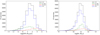 |
Fig. 1. Distributions of SFRs (left) and of stellar masses (right) of source populations in our sample, subdivided into SFGs, RL, and RQ AGN. The distribution of SFRs of RL AGN extends to very low values, consistent with the fact that their radio emission is unrelated to the SFR; especially in the nearby universe they are generally associated with passive ellipticals. Both RQ and RL AGN preferentially reside in massive galaxies, with median stellar masses significantly higher than the mean stellar mass of SFGs. See text for more detailed comments. |
RL AGN have the broadest distribution of SFRs, with a substantial tail extending to very low values, as expected since, especially at low z, they are frequently associated with evolved early-type galaxies; their median is log(SFR/M⊙ yr−1) = 0.92 with standard deviation σlog(SFR) = 1.46. On the contrary, the SFR distribution of RQ AGN is shifted towards the highest values: median log(SFR/M⊙ yr−1) = 2.33 with standard deviation σlog(SFR) = 0.90. SFGs have a median log(SFR/M⊙ yr−1) = 1.59 with a standard deviation σlog(SFR) = 0.81. The median stellar masses of all source populations are quite large: log(M⋆/M⊙) = 11.05, 11.17, and 10.89, for RL AGN, RQ AGN, and SFGs, respectively; the corresponding standard deviations are 0.43, 0.59, and 0.51, respectively.
These median values vary with redshift. In the case of RL AGN the median log(SFR/M⊙ yr−1) increases from −0.16 at z = 0.5, to 0.70 at z = 1, to 1.67 at z = 2; the corresponding dispersions are 0.63, 0.61, and 0.42, respectively. The relatively low dispersion at the highest redshift reflects the fact that at high-z most RL AGN are hosted by SFGs while the fraction of passive hosts is large at low z. Instead, the median log(M⋆/M⊙) is quite stable; at the aforementioned redshifts it takes the values of 11.02, 11.09, and 11.00 with dispersions of 0.38, 0.33, and 0.44, respectively.
The increase with redshift of the mean SFR is somewhat less steep for RQ AGN and for SFGs, compared to RL AGN. At the same three redshifts, the median log(SFR) is 0.95 (0.34), 1.53 (0.36) and 2.29 (0.34) for RQ AGN (standard deviations in parenthesis); for SFGs it is 1.02 (0.28), 1.58 (0.28) and 2.20 (0.27). At variance with RL AGN, also the median log(M⋆) of RQ AGN and SFGs increase with redshifts. For RQ AGN we have log(M⋆) = 10.75 (0.40), 10.95 (0.42) and 11.20 (0.42). For SFGs, log(M⋆) = 10.68 (0.32), 10.92 (0.30) and 11.12 (0.36). The specific SFR (sSFR) of SFGs increases from ≃0.22 Gyr−1 at z = 0.5 to ≃0.66 Gyr−1 at z = 1, to ≃0.83 Gyr−1 at z = 2. The evolution of the sSFR with redshift is substantially shallower than found, in this redshift range, by several previous studies (e.g., Whitaker et al. 2014; Speagle et al. 2014; Johnston et al. 2015; Lehnert et al. 2015, sSFR ∝ (1 + z)p with p in the range 2.6–3) but consistent with the results by Schreiber et al. (2015) and Bourne et al. (2017, for the sSFR derived from IR+UV data), p ≃ 1.5–1.6.
The redshift distribution of each source sub-population is shown in Fig. 2. The median redshift is ∼1.06. The AGN fraction of detected sources increases with increasing redshift. Duncan et al. (2021) mention the possibility of selection effects in the spectroscopic sample used for photo-z training. They also caution that the limited number of spectroscopic redshifts at z > 1 results in a deterioration of the quality of photometric redshift estimates for host-dominated sources in the range 1 < z < 1.5, and the quality becomes substantially worse for z > 1.5.
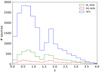 |
Fig. 2. Redshift distributions of sources in our sample, subdivided into SFGs, RL and RQ AGN. Most redshifts, especially at z > 1, are photometric. Their quality deteriorates for z > 1.5 and the distributions at z > 4 are unreliable. We have therefore cut them off at z = 4. See text for a comment on the origin of the dip at z ≃ 1.3. |
The origin of the dip at z ∼ 1.3 can be largely ascribed to aliasing effects in the photo-z distribution. The photo-z’s were fixed at the median of the first photometric redshift solution, and for reasons associated with the filter wavelength distribution, this seems to disfavour redshifts z ∼ 1.3 for both SFGs and RL AGN and instead alias them to slightly higher or lower redshifts. We note, incidentally, that the very small fraction of spectroscopic redshifts at z > 1 implies that our redshift distribution is not biased by the ‘redshift desert’, namely by the lack of strong spectroscopic features detectable from the ground for galaxies in the redshift range z ∼ 1.4–2.5 (e.g., Steidel et al. 2004).
On the other hand, a feature in the redshift distribution of SFGs at z ∼ 1.5 is expected since the dominant population of SFGs changes around this redshift: below z ∼ 1.5 SFGs are mostly late-type while at higher redshifts we enter the era when early-type galaxies formed the bulk of their stars (Cai et al. 2013). Hints of a dip at z ∼ 1.5 can be discerned in the redshift distribution for S1.4 GHz > 50 μJy (not far from the effective depth of the LoTSS survey) predicted by Mancuso et al. (2015). According to the model, the dip is caused by the fact that, at z ≃ 1.5, the rapid drop of the star-formation activity of proto-spheroidal galaxies, which formed most of their stars at higher redshifts, is only partly compensated by normal late-type and starburst galaxies, which dominate the star formation at lower redshifts. Since the radio luminosity functions of proto-spheroidal and of late-type and starburst galaxies are substantially different, the presence or absence of the dip depends on the luminosity corresponding to the flux density limit of the survey at z ≃ 1.5; in other words, the presence or absence of the dip depends on the flux density limit.
3. Results
3.1. Comparison with an independent 1.4 GHz based source classification
Bonato et al. (2021) studied a sample of 1173 sources brighter than S1.4 GHz = 120 μJy, namely with a signal-to-noise ratio ≥10, in the central ≃1.4 deg2 of the ≃6.6 deg2 area covered by the WSRT survey in LH field by Prandoni et al. (2018); the synthesised beam is of 11″×9″ with position angle PA = 0°. Thus this sample covers an area about a factor of seven smaller than that covered by the present LOFAR sample. SFRs were taken, when available, from the Herschel Extragalactic Legacy Project (HELP) catalogue (Shirley et al. 2019); otherwise the 24 μm flux density was used as a SFR indicator (Battisti et al. 2015).
The HELP SFRs were obtained via SED fitting with CIGALE (Małek et al. 2018). HELP collates, heals and homogenises multi-frequency data over the 1270 deg2 covered by the Herschel SPIRE extragalactic surveys. The surveys covering each Herschel field are highly variable in number, wavebands and depth. For the WSRT LH field, HELP contains optical photometry in the g, r, i, z, and y bands and near-IR photometry in the K band and in Spitzer IRAC bands, in addition to Herschel data. CIGALE was run for all HELP galaxies with at least two optical and at least two near-IR detections (Shirley et al. 2021). The code estimates the galaxy properties by SED fitting. Model SEDs are computed dealing self-consistently with stellar emission and its reprocessing by dust.
For the comparison with the classification based on the LOFAR flux densities, we redid the classification after rescaling the WSRT flux densities by a factor of 0.84 in order to bring them to statistical agreement with the multi-frequency radio measurements in the same field (see Paper II; their Fig. D.1). This has led to some differences with the original classification by Bonato et al. (2021). Apart from that, the classification was done using the same criteria. If an estimate of the SFR was available, sources were classified as RL AGN if their L1.4 GHz/SFR ratios exceeded the redshift-dependent threshold derived by Delvecchio et al. (2017). Otherwise, the criterion by Magliocchetti et al. (2017), based on radio luminosity, was adopted. Non-RL AGN sources were classified as either SFGs or RQ AGN using the diagnostics, based on near and mid-IR colours, by Messias et al. (2012) or by Donley et al. (2012), depending on the available data. The classification was tested by exploiting the X-ray data from the XMM-Newton survey by Brunner et al. (2008), which extends over ≃10% of the field covered by the Bonato et al. (2021) sample.
Most of the WSRT sources (1004/1173 ≃ 86%) have a LOFAR counterpart within 3.5 arcsec, corresponding to 3 times the quadratic sum of WSRT (Prandoni et al. 2018) and LOFAR (Kondapally et al. 2021) rms positional uncertainties, ≃1″ and ≃0.6″, respectively. The WSRT astrometric error refers to the 5 σ flux density limit; the LOFAR error is a conservative empirical estimate. The surface densities of the WSRT sample studied by Bonato et al. (2021) and of the present LOFAR sample are ≃6.46 × 10⁻⁵ arcsec−2 and ≃2.33 × 10⁻⁴ arcsec−2, respectively. In the absence of further information, the expected number of chance associations within 3.5 arcsec would be ≃10.5 (≃0.9%). However, in making the WSRT/LOFAR associations, we also took into account the optical-to-near-IR identifications, which have substantially better positional accuracy. In this way the number of chance associations becomes negligible.
It is interesting to compare the classifications by Bonato et al. (2021) with those by Paper V. The WSRT–based classification of the 1004 common sources yielded 392 RL AGN, 306 SFGs, 131 RQ AGN and 175 unclassified. The LOFAR–based classification yielded 379 RL AGN, 493 SFGs, 93 RQ AGN and 39 unclassified. The two classifications agree for 86% of sources classified as non-RL AGN, demonstrating a remarkable stability against variations of the classification criteria. The situation is trickier in the case of RL AGN. Only ≃69% of sources classified in this way by Bonato et al. (2021) have the same classification in Paper V; about 26% of sources become SFGs or RQ AGN while the remaining ≃5% are unclassified.
Some classification discrepancies are expected because of differences in the classification criteria (50 out of the 104 LOFAR-unconfirmed WSRT RL AGN were classified using the criterion by Magliocchetti et al. 2017), in estimates of the SFRs (also due to different input photometry) and because of the different radio excess threshold. However, since the adopted thresholds are quite similar, the most likely culprit at least for a fraction of sources is a difference in the radio luminosity to SFR ratio between 1.4 GHz and 150 MHz, compared to the expectation for the average spectral index. We therefore investigated the spectral index distributions. They are shown in the left-hand panel of Fig. 3. The median spectral index for the full sample is −0.70. The median spectral indices of the various populations are close to each other: −0.72, −0.68, and −0.74, respectively, for sources classified as RL AGN, RQ AGN and SFGs by both Bonato et al. (2021) and Best et al. (in prep.). The median spectral index of non-RL AGN (i.e. SFGs plus RQ AGN) is −0.73.
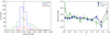 |
Fig. 3. Left panel: spectral index distributions of the 3 source populations. The median spectral indices (vertical lines) are: −0.72 for RL AGN, −0.74 for SFGs and −0.68 for RQ AGN. Right panel: redshift dependence of the median spectral indices of sources classified as RL AGN (filled green triangles) and as non-RL AGN (i.e. as SFGs or RQ AGN; filled blue circles) based on both WSRT and LOFAR data. The filled black diamonds (‘TOT’) represent the median values for the full set of WSRT sources with LOFAR counterparts, including those with different classifications and the unclassified ones. Error bars are the interquartile ranges divided by the square root of the number of objects in the bin. A slight trend towards a steepening of the spectral index with increasing z is visible, especially in the case of RL AGN, but its statistical significance is low (see text). |
Sources classified as RL AGN by Bonato et al. (2021) but not by Best et al. (in prep.) have a substantially flatter median spectral index (−0.55, corresponding to a difference of about 0.15 dex in 150 MHz radio luminosity), implying lower L150 MHz/SFR ratios than expected based on the median spectral index of the full sample. They can thus fall below the threshold for classification as RL AGN. In fact we find that in most cases the origin of the different classification can be traced back to this effect. A similar conclusion applies to the 47 WSRT RL AGN without a LOFAR counterpart3.
It should be noted that the impact of this problem on our analysis is modest. In fact, RL AGN comprise a minor fraction of our sources; they are only 22% of non-radio excess sources. Thus, even in the worst case the number of SFGs plus RQ AGN would have been overestimated by 0.27 × 0.22 ≃ 6%. However, the fact that these sources fall below the threshold for the classification as RL AGN at 150 MHz means that, at this frequency, a significant fraction, probably the majority, of the radio emission is due to star formation. Hence, the comparison between the abundances of different source populations measured at different frequencies requires some caution. In the following we use the classification by Best et al. (in prep.).
The right-hand panel of Fig. 3 shows an indication of a flattening of the median spectral index of RL AGN at the lowest redshifts. The indication is only marginally significant (at the ≃95% confidence level, based on Pearson’s correlation coefficient) for our sample, but a similarly flat spectral index of low-z AGN was reported by Calistro Rivera et al. (2017, their Fig. 10) for a brighter sample, although they found a steepening of the AGN spectral index between 150 and 325 MHz. Apart from that, the figure shows a slight trend towards a steepening of the AGN spectral index with increasing z. This kind of trend has long been known, although its origin is not well understood (see Miley & De Breuck 2008, for a review). The statistical significance of the redshift dependence is, however, low (the probability of an occurrence by chance is 0.01, corresponding to 2.57 σ), consistent with the earlier conclusions by Calistro Rivera et al. (2017).
3.2. Radio luminosity versus SFR
Figure 4 displays the 150 MHz radio luminosity versus SFR for our sample. The cyan points identify the ‘SFG region’ (including RQ AGN). Some sources that were classified as RL AGN on the basis of clearly extended radio emission (i.e. jets) turned out to be located within the SFG region. They could be radio-loud AGN where the radio excess just does not quite make the 0.7 dex threshold or RQ AGN, as they can also have jets, and have been reclassified as such. These objects are a tiny fraction of sources, and their reclassification does not significantly affect our results.
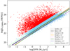 |
Fig. 4. Radio luminosity at 150 MHz versus SFR. Red and cyan points represent, respectively, RL AGN and non-RL sources (i.e. SFGs plus RQ AGN). The black solid line shows the ridge line in the radio–SFR relation used by Best et al. (in prep.) to define the radio excess threshold (0.7 dex above the ridge line) separating RL AGN from SFGs plus RQ AGN. Also shown, for comparison, are the relations by Smith et al. (2021, grey dashed line), by Gürkan et al. (2018, brown dotted line), Bonato et al. (2017, non-linear model; dark green solid line), Delhaize et al. (2017, dark blue dashed line), Brown et al. (2017, orange solid line), Calistro Rivera et al. (2017, light green dotted line) and Murphy et al. (2012, pink dashed line). |
The solid black line is the ridge line in the radio–SFR relation used by Best et al. (in prep.) to define the radio excess threshold separating RL AGN from SFGs and RQ AGN. It is given by log(SFR) = 0.93(log L150 MHz − 22.24) with SFR in M⊙ yr−1 and L150 MHz in W Hz−1. The use of the ridge line mitigates the effect of the radio selection, which biases the mean or median values towards brighter radio sources. As mentioned above the upper bound of the SFG region is set at L150 MHz 0.7 dex above the ridge line.
The figure also shows, for comparison, the stellar mass-independent relations presented by Smith et al. (2021), Gürkan et al. (2018), Brown et al. (2017), Delhaize et al. (2017), Calistro Rivera et al. (2017), Bonato et al. (2017, non-linear model), and Murphy et al. (2012). The Smith et al. mass-independent relation was derived for a near-IR selected sample of z < 1 galaxies using the LOFAR survey data over the ELAIS-N1 field. The SFRs were obtained from MAGPHYS alone, rather than from the combination of SED fitting methods used by Best et al. (in prep.). To avoid the bias related to the radio selection, Smith et al. (2021) used all estimates of L150 MHz, irrespective of their statistical significance, since they showed that censoring the sample could affect the derived SFR/L150 MHz relation. The resultant relation is in fairly close agreement with the ridge line of Best et al. (in prep.).
The relations presented by Gürkan et al. (2018) and by Calistro Rivera et al. (2017) are based on shallower LOFAR surveys. The former authors exploited a sample selected from the seventh data release of the Sloan Digital Sky Survey (SDSS DR7; Abazajian et al. 2009) catalogue over the Herschel Astrophysical Terahertz Large Area Survey (H-ATLAS; Eales et al. 2010) North Galactic Pole (NGP) field (Maddox et al. 2018), which overlaps with the LoTSS DR1 (Shimwell et al. 2017). Star-formation rates and stellar masses were computed using MAGPHYS. In Fig. 4 we show their single power-law fit, although they also derive a stellar-mass-dependent relation.
Calistro Rivera et al. (2017) investigated the IR-radio correlation at both 150 MHz and 1.4 GHz of radio selected SFGs over the LOFAR Boötes field (Williams et al. 2016). The source classification and the determination of their physical parameters were performed using the SED-fitting algorithm AGNfitter. The IR-radio correlation was found to be redshift-dependent. The line shown in Fig. 4 refers to the median redshift of our sample (z = 1.06).
The study by Delhaize et al. (2017) relies on the high-sensitivity VLA observations at 3 GHz in the COSMOS field. Luminosities at 1.4 GHz were computed using the individual spectral indices when available or α = −0.7 otherwise. SFRs were derived from total IR luminosities using the conversion by Kennicutt (1998) assuming a Chabrier (2003) IMF. We extrapolated their infrared-to-radio luminosity ratio at 1.4 GHz to 150 MHz by setting α = −0.7. A slight decrease in such a ratio with increasing redshift was reported by Delhaize et al. (2017). Again, the line shown in Fig. 4 refers to z = 1.06.
Murphy et al. (2011) calibrated the 1.4 GHz radio luminosity versus SFR relation using Starburst99 (Leitherer et al. 1999) for a Kroupa (2001) IMF in combination with some empirical recipes. Bonato et al. (2017) computed the local radio luminosity function at 1.4 GHz by convolving the observationally determined local SFR function (Mancuso et al. 2015) with a power-law dependence of L1.4 on the SFR. The parameters of the L1.4–SFR relation were derived by fitting the local 1.4 GHz luminosity function of SFGs (Mauch & Sadler 2007). The Murphy et al. and Bonato et al. relations were extrapolated to 150 MHz using the thermal and non-thermal spectral indices quoted in the respective papers.
As illustrated by Fig. 4, there are differences among the relations, both in slope and in normalisation. The variations in the L150 MHz/SFR ratios can reach a factor > 2 (cf. Sect. 1).
It can be noted that, at low SFRs, the relation from Paper V (black solid line in Fig. 4) lies below the average value of detected sources. This is due to having adopted the ridge line instead of the mean to minimise the effect of radio selection.
Figure 5 shows the mode of the distribution of SFR/log(L150 MHz) ratios of SFGs plus RQ AGN (data points) as a function of stellar mass for four redshift bins. The error bars are simply the interquartile ranges within each bin. These are intended to give an indication of the range of values: A proper error estimate would involve taking into account the probability distributions of the photometric redshifts, and uncertainties on consensus stellar masses and SFRs, which is beyond the scope of this paper. Furthermore, the measured values are potentially affected by systematic factors, such as the radio flux density limits.
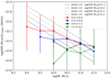 |
Fig. 5. Ratio of the radio luminosity at 150 MHz to the SFR as a function of M⋆ of SFGs plus RQ AGN for four redshift bins. The points are the modes of the distributions of log(SFR/L150 MHz). The error bars are the interquartile errors. The straight lines show, for comparison, the relations derived by Smith et al. (2021) for 4 values of the SFR. Although these relations are steeper than ours, the agreement is good for SFGs with typical properties, i.e. where we have more data, both globally and for each redshift bin (see text). |
We see a slight trend towards a lower SFR/log(L150 MHz) ratio with increasing M⋆ at z ≲ 1. This trend is not seen at higher redshifts, and may even be reversed in the bin 1.5 < z < 2.5. The trend is substantially weaker than those reported by Smith et al. (2021) for z < 1, and by Delvecchio et al. (2021) for 0.1 < z < 4.5. These authors find, respectively, a decrease of 0.33 ± 0.04 and of 0.234 ± 0.017 per decade of M⋆ above log(M⋆/M⊙) = 10 while our data indicate a decrease ≲0.1.
These differences reflect the different primary selection. Our radio selection favours higher radio luminosities for a given SFR, hence lower log(SFR/L150 MHz). This selection bias is increasingly important for lower mass galaxies, which are expected to have lower SFRs and hence lower radio luminosities; this leads to an increasing fraction falling below the radio flux density limit and hence a potential bias in the measured value of log(SFR/L150 MHz) as only the objects with the brightest L150 MHz for a given SFR are detected. It may well account for the flatter slope of the log(SFR/L150 MHz) versus M⋆ relation compared to those found by Smith et al. (2021) and Delvecchio et al. (2021), who started from near-IR and from M⋆–selected samples, respectively. We note that, even though these two selections are similar in that they favour higher M⋆/SFR ratios, they still lead to significantly different relation. This is another manifestation of the importance of selection effects. However, we are in good agreement with the results by Smith et al. (2021) where we have more data, namely for SFGs with typical properties in each redshift bin. This can be seen considering the peaks of our distributions of SFRs and of stellar masses: they occur at SFRs of 1.1, 9.2, 29.4, 83.1 M⊙ yr−1 and log(M⋆/M⊙) = 10.49, 10.80, 11.04, 11.12 for 0 < z < 0.4, 0.4 < z < 0.8, 0.8 < z < 1.5, 1.5 < z < 2.5, respectively. The peaks of the global distributions occur at log(M⋆/M⊙)≃11, z ∼ 1, log(SFR/M⊙ yr−1)≃1.6.
Figure 5 also shows an indication of a decrease in the log(SFR/L150 MHz) ratio with increasing redshift, except for the largest stellar masses. In terms of qTIR ∝ (1 + z)δ we find δ ≃ −0.12 for log(M⋆/M⊙)≃10.5, comparable to the values reported by Delhaize et al. (2017, δ = −0.19 ± 0.01), by Magnelli et al. (2015, δ = −0.12 ± 0.04) and by Calistro Rivera et al. (2017, δ = −0.22 ± 0.05, at 150 MHz). The evidence for a redshift evolution progressively weakens with increasing M⋆ and becomes insignificant for log(M⋆/M⊙)≳11. We caution, however, that the higher redshifts are more likely to suffer from the biases discussed above. Our results are consistent with the conclusion by Smith et al. (2021) and Delvecchio et al. (2021) that the cosmic evolution of the SFR/L150 MHz ratio is mostly driven by its decrease with increasing M⋆, coupled with the fact that the effective M⋆ of radio-selected SFGs increases with redshift (see the upper panel of Fig. 3 of Smith et al. 2021).
Figure 6 presents a different view of our data by showing them in terms of the specific SFR (sSFR) as a function of M⋆. There is a clear decrease in the sSFR with increasing M⋆ except perhaps in the lowest redshift bin. A similar trend was reported by Bourne et al. (2017) who used the deepest 450– and 850–μm imaging from SCUBA-2 Cosmology Legacy Survey. Our results are consistent with theirs, within the errors of both estimates, in the overlapping redshift range (0.5 < z < 2), although our data hint at an excess sSFR of the lowest stellar masses. If real, the excess may be due to a higher efficiency of the radio selection at detecting early phases of galaxy evolution, when the stellar masses were still relatively low. Our data do not show the flattening of the slope of the log(sSFR) versus log(M⋆) relation at low M⋆ reported by Whitaker et al. (2014) for their near-IR selected sample. This can be another indication that the optical and near-IR selection underestimates the SFR of dust-enshrouded galaxies in their early evolutionary phases. As pointed out above, the redshift evolution of the amplitude of the log(sSFR) versus log(M⋆) relation implied by our data is consistent with the results by Bourne et al. (2017) but is substantially weaker than found by Whitaker et al. (2014) and by other surveys (cf. Sect. 2.2).
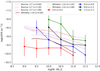 |
Fig. 6. Specific SFR of our SFGs plus RQ AGN as a function of M⋆ for 4 redshift bins. The lines show the analytic models by Whitaker et al. (2014) and Bourne et al. (2017), fitting their data, computed at the median redshifts of our bins (z = 0.60, 1.05 and 1.89). Our lowest redshift bin is outside the range covered by the other studies. |
3.3. SFR versus stellar mass
The correlation between SFR and M⋆ for SFGs, known as the ‘main sequence’ (MS), has been extensively discussed in the literature (e.g., Noeske et al. 2007; Elbaz et al. 2007; Rodighiero et al. 2014; Schreiber et al. 2017; Santini et al. 2017; Bera et al. 2018; Gu et al. 2019; Leslie et al. 2020, and references therein). The shape of this correlation was found to vary depending on the sample selection. Figure 7 shows the distribution in the log(SFR)−log(M⋆) plane of our SFGs in the 1.5−2.5 redshift range studied by Rodighiero et al. (2015), a reference paper for the definition of the main sequence. The correlation between the two quantities is weak, as also found for sub-mm selected galaxies (e.g., Michałowski et al. 2012; Koprowski et al. 2016).
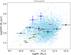 |
Fig. 7. Distribution in the SFR–M⋆ plane of our SFGs and RQ AGN in the 1.5 ≤ z ≤ 2.5 redshift interval (cyan points). The black filled circles with error bars show the modes of the SFR distributions averaged over the stellar mass bins represented by horizontal bars. The numbers of sources in each bin, from low to high M⋆, are 93, 511, 1511, 2491, 1001, and 50, respectively. The vertical bars show the dispersions. The red symbols represent the average values for the Rodighiero et al. (2015)K-band selected sample of SFGs. The upper blue points show the average SFRs for the Rodighiero et al. (2015) sample of starburst galaxies in their two mass bins. The green asterisks represent the Leslie et al. (2020) median values for their SFG sample (light green for their 1.5–2 redshift range, dark green for 2–2.5). |
Our radio-selected sample has an average SFR/M⋆ ratio similar to that of the K-band selected sample of SFGs investigated by Rodighiero et al. (2015) for log(M⋆/M⊙)∼11. At lower stellar masses our objects have substantially higher ratios, as expected since our selection favours objects with high SFRs while the optical selection favours lower SFR/M⋆ ratios. Above log(M⋆/M⊙)∼11 our average SFR/M⋆ ratios are below the extrapolation of the Rodighiero et al. (2015) relation, but consistent with, or slightly larger than the mean ratios reported by Leslie et al. (2020) for the VLA-COSMOS 3 GHz Large Project sample at z ≲ 2.5, where the overwhelming majority of our SFGs reside. This is in agreement with the flattening and bending of the SFR–M⋆ relation at large stellar masses reported by several authors (e.g., Schreiber et al. 2015; Tomczak et al. 2016) and investigated in great detail by Leslie et al. (2020).
The distribution of SFRs of galaxies in our sample reaches substantially higher values than the deep K-band selected sample by Rodighiero et al. (2015), seamlessly extending over the region of ‘starburst’ galaxies that do not appear as a distinct group. In other words, our radio selection does not underscore any clear correlation between SFR and M⋆. Such a correlation arises when SFGs have grown a sufficiently large stellar mass to allow an optical selection. The radio and the FIR and sub-mm selections are insensitive to the stellar mass and therefore yield samples covering a very wide range of M⋆/SFR ratios.
Our radio selection provides a view of the distribution of galaxies in the SFR–M⋆ complementary to that of optical selection. The latter emphasises M⋆ while the radio (and the far-IR and sub-mm) selection hinges upon the SFR. To be more specific, at high stellar masses, the radio selection picks out objects that are beginning to quench (below the main sequence) and yet still have sufficient SFR to be detected; these are classified as SFGs in the current analysis because they have no AGN activity, but in typical optical selections they are excluded from main sequence analyses as ‘quenched’ galaxies. At lower masses, the radio observations do not have the sensitivity to probe the typical objects seen on the mass-selected main sequence; instead the radio sample is dominated by objects above the main sequence (starbursting, or just randomly high). This gives a different picture.
Both views must be taken into account in order to properly understand the star-formation history of galaxies. For example, the distinction between MS and ‘off-sequence’ galaxies, frequently found in the literature (e.g., Rodighiero et al. 2011, 2015; Silverman et al. 2015; Schreiber et al. 2015), tends to be interpreted as indicative of two different modes of star formation: a secular star-formation mode of galaxies within the MS and a stochastic star-formation mode with strongly enhanced star-formation efficiency, perhaps triggered by major mergers for off-sequence galaxies (e.g., Elbaz et al. 2018).
However, the fact that the radio selection does not show any clear sequence suggests a higher uniformity of the star-formation history of galaxies, with the MS corresponding to a long-lived phase of galaxy evolution, with a well developed stellar population, most easily picked up by the optical and near-IR selection. Instead, the radio (and far-IR and sub-mm) selection sees the full history of star formation, from the initial phases when the stellar masses were very low (i.e. the SFR/M⋆ ratios were well above the main sequence) to later phases when these ratios take on MS values.
3.4. Radio luminosity functions
The luminosity of a source with flux density Sν is
 (1)
(1)
dL being the luminosity distance and K(Lν, z) the K-correction,
![Mathematical equation: $$ \begin{aligned} K(L_\nu ,z)=\frac{(1+z)L[\nu (1+z)]}{L(\nu )}. \end{aligned} $$](/articles/aa/full_html/2021/12/aa41286-21/aa41286-21-eq3.gif) (2)
(2)
We have assumed simple power-law spectra, Sν = να, so that K = (1 + z)1 + α. We used the median value of the 1.4 GHz–150 MHz spectral index (-0.73) derived from non-RL AGN sources (SFGs and RQ AGN) with counterparts in the WSRT survey (see Sect. 3.1).
The luminosity function (LF) in the k-th redshift bin was derived using the 1/Vmax method (Schmidt 1968):
 (3)
(3)
where zk is the bin centre and the sum is over all the Nj sources with luminosity in the range [log Lj − Δ log L/2, log Lj + Δ log L/2] within the redshift bin. We chose Δz = 0.2 for z < 2 and Δz = 0.4 for z > 2. These redshift bins are large enough to have sufficient statistics and narrow enough to allow us to neglect evolutionary corrections within the bin. The values of Δ log L are different in different redshift bins (see Table A.1); they are larger in the poorly populated luminosity ranges.
The Vmax, i is the comoving volume within the solid angle of the survey enclosed between the lower limit, zmin, of the bin and the minimum between the upper limit, zmax, and the maximum redshift at which the source is above the radio flux-density limit that we assumed, namely Slim = 145 μJy. The weights wi include corrections for incompleteness in the radio source catalogue due to the variable rms noise across the survey area, in classification and in redshift. Incompleteness in source counts was corrected using the factors estimated by Mandal et al. (2021), as explained in Sect. 2.1. Mandal et al. (2021) estimated the resolution bias correction based on an integrated source size distribution, which is the result of the relative contribution of (more compact) SFGs and (more extended) RL AGN as a function of flux density. We caution that in principle this may result in not fully appropriate corrections to SFG LFs at flux densities where RL AGN dominate. We notice however that significant resolution bias corrections only apply at flux densities fainter than 0.3–0.4 mJy, where the radio catalogue is strongly dominated by SFGs and hence the integrated source size distribution is SFG-like. At higher flux densities the corrections are negligible.
The completeness in the classification or in redshift for each bin of log(S150 MHz) was estimated as the ratio between the number of classified sources, or of sources with reliable redshift, and the total number of sources in such a bin. While acknowledging that this procedure is not ideal, we note that our results are very weakly sensitive to corrections for these incompletenesses since ≈97.6% of our sources are optically identified and ≈96.9% have either spectroscopic or reliable photometric redshift (see Sect. 2.1).
The Poisson error on dN(Lj, zk)/dlog L was estimated as:
![Mathematical equation: $$ \begin{aligned} \sigma _{j,k} = \left\{ \sum _{i=1}^{N_{j}} \frac{{ w}_{i}^{2}}{[V_{\mathrm{max},i}(z_k)]^{2}}\right\} ^{1/2}. \end{aligned} $$](/articles/aa/full_html/2021/12/aa41286-21/aa41286-21-eq5.gif) (4)
(4)
Our estimates of the 150 MHz LFs for SFGs and RQ AGN are listed in Table A.1. Figure 8 displays such LFs for some representative redshifts and compares them with several estimates found in the literature.
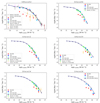 |
Fig. 8. Comparison of our estimates of the 150 MHz luminosity functions (LFs) of non-radio excess sources (SFGs and RQ AGN) at representative redshifts with those of SFGs (including RQ AGN) from the T-RECS simulations (Bonaldi et al. 2019). Our LFs are also compared with the LF estimates at 1.4 GHz by Butler et al. (2019), Novak et al. (2017), Padovani et al. (2015) and Mauch & Sadler (2007), and at 610 MHz by Ocran et al. (2020), all scaled to 150 MHz using a spectral index α = −0.73. The local (0.05 ≤ z ≤ 0.2) LFs are also compared with the Wilman et al. (2008) model for SFGs and RQ AGN. The error bars are the quadratic sums of Poisson uncertainties and of sample variance; they are generally smaller than the symbols. The real uncertainties are much larger, especially at z > 1 where the quality of photometric redshifts increasingly worsens, but are difficult to quantify. |
The error bars take into account also the sample variance, in other words, the field-to-field variations in the source number density. According to Eq. (8) of De Zotti et al. (2010)  , N being the mean number density of sources in the bin and Ω the survey area (Ω = 10.28 deg2 in our case). The global error is thus the sum in quadrature of Poisson and sample variance errors.
Our sample has allowed us to determine the luminosity functions at 150 MHz of both SFGs and RQ AGN in the local universe (z ≃ 0.1) over about four decades in luminosity. The results are generally in good agreement with the local luminosity function at 1.4 GHz measured by Mauch & Sadler (2007) and, specifically for the SFG population, with the Butler et al. (2019), Novak et al. (2017) and Ocran et al. (2020) observational estimates. Also good is the agreement with the T-RECS (Bonaldi et al. 2019) and the Wilman et al. (2008) simulations of SFGs. However, below the knee luminosity our local LF is somewhat steeper than the Mauch & Sadler (2007) and T-RECS ones. This matches the slightly higher sub-mJy counts (the bump between 0.25 and 0.8 mJy) measured by Mandal et al. (2021) compared to the T-RECS simulations. The deficiency of simulated sources is mostly associated with low redshifts.
Our estimates of the RQ AGN LFs are generally lower than those by Padovani et al. (2015) and than the simulations by Wilman et al. (2008). We agree with Padovani et al. (2015) and with Bonato et al. (2021) that the RQ AGN fraction is higher at the highest radio luminosities (log(L150 MHZ/W Hz−1) ≳ 24). This might mean that RQ AGN are associated with the most powerful starbursts, although some residual AGN contamination cannot be ruled out. Our estimates reach down to the knee luminosity up to z ≃ 0.5. At higher redshifts our sample probes only the highest radio luminosities. The consistency with the T-RECS simulations remains good although there are hints of incompleteness in our lowest luminosity bins.
3.5. Star-formation rate functions
The SFR functions of SFGs and RQ AGN were computed by convolving their radio LFs with the distributions of the SFR/L150 MHz ratios at given L150 MHz. We used a Monte Carlo approach, carrying out 100 000 simulations to sample the distribution of the SFR/L150 MHz ratios as a function of L150 MHz. The distribution was modelled as a Gaussian with a mean given by the log(L150 MHz)–log(SFR) relation by Best et al. (in prep.); the dispersion around the mean relation was found to be 0.282.
The results for each population and their sum are listed in Table A.2 and displayed in Fig. 9 for a set of representative redshifts. The effective numbers of sources given in the table are the number of sources corresponding to the central values of the SFR function: since it was determined via Monte Carlo simulations, there is no unique number of sources in each bin. Estimates of the SFR functions of SFGs in their two highest redshift bins (⟨z⟩ = 3.7 and 4.8) were worked out by Novak et al. (2017).
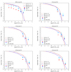 |
Fig. 9. Comparison of our observational estimates of the SFR functions with the theoretical ones by Mancuso et al. (2015, blue dashed lines), Aversa et al. (2015, red dotted lines) and Mancuso et al. (2016, brown dashed lines). The lines can be seen as representations of observational estimates of the SFR functions based on combinations of classical UV and FIR star-formation tracers (see text). They indicate that the LoTSS data allow us to measure space densities of typical high-z SFGs, with SFR ∼ 100 M⊙ yr−1, up to z ≃ 2.5. The two inflection points, at log(SFR/M⊙ yr−1)≃1 and ≃3.5, of the Mancuso et al. (2015) line for z > 1.5 correspond to the transition from the dominance of late-type galaxies to that of star-forming protospheroids and to the dominance of strongly lensed galaxies, respectively. The error bars are the quadratic sums of Poisson uncertainties and of sample variance; they are generally smaller than the symbols. The real uncertainties are much larger, especially at z > 1 where the quality of photometric redshifts increasingly worsens, but difficult to quantify. |
Figure 9 also shows, for comparison, analytic fits of estimates of the global SFR functions by Mancuso et al. (2015, 2016), and Aversa et al. (2015), all based on FIR, sub-mm, optical and UV data. In fact, the lines in this figure can be seen as representations of data from such spectral regions.
Mancuso et al. (2015) complemented the SFR functions yielded by the Cai et al. (2013) model that fitted a broad variety of IR data on dust-obscured star formation over a wide redshift range, with a parametric model for the unobscured star formation, successfully tested against the observed Hα and UV luminosity functions. Aversa et al. (2015) described the bolometric luminosity due to star formation as the sum of UV plus IR luminosities in such proportions that the observed LFs in both bands at all redshifts are reproduced. Whenever insufficient data were available, the SFR functions were constrained using the continuity equation to link them to the halo mass function. Mancuso et al. (2016) performed educated minimum–χ2 fits of IR and dust-corrected data assuming a Schechter shape for the SFR functions, with redshift-dependent parameters.
Our observational estimates are in reasonably good agreement with the results by Mancuso et al. (2015) but are generally below those by Mancuso et al. (2016) and even more below those by Aversa et al. (2015). The inflection points of the Mancuso et al. (2015) function at z > 1.5 correspond to the changes of the dominant population according to the Cai et al. (2013) model. At low z the dominant population is made of normal and starburst late-type galaxies, while at z > 1.5 proto-spheroidal galaxies and bulges in the process of forming the bulk of their stars take over above log(SFR/M⊙ yr−1)≃1 (first inflection point). Strongly lensed galaxies account for the highest (apparent) SFRs, above log(SFR/M⊙ yr−1)≃3.5 (second inflection point). Figure 9 shows that our sources do not reach the extreme values of the SFR where strongly lensed galaxies are predicted to dominate. Their maximum SFRs are in the range of unlensed hyperluminous infrared galaxies (HyLIRGs) with SFR ≳ 1000 M⊙ yr−1 (Fu et al. 2013; Ivison et al. 2013). However, source blending (e.g., Hayward et al. 2013) and AGN contributions to the IR luminosity used to derive the SFR (a large fraction of the highest-SFR galaxies host a RQ AGN, see Fig. 9) can also have a role.
It is remarkable that radio data alone have allowed us to derive SFR functions in broad agreement with those based on a complex combination of UV to optical to IR data. The differences can be accounted for by the still substantial uncertainties on the calibration of recipes for deriving the SFR from data in the various wavebands. The comparison with representations of data from classical SFR measures shows that the LoTSS survey is deep enough to allow the determination of space densities of typical SFGs (with SFR at the knee of the function, SFR ∼ 100 M⊙ yr−1) up to z ≃ 2.5. SFGs not hosting AGN dominate the global SFR functions although the contribution of AGN hosts increases with increasing SFR.
4. Conclusions
We have exploited the unprecedented sensitivity of LoTSS Deep Fields survey of the Lockman Hole field to investigate the relation between radio emission and SFR in SFGs. The LH field is exceptionally well suited for this purpose given the wealth of multi-frequency data available on radio-detected sources. Of the 31,162 sources in the final LH cross-matched catalogue, 97.6% have multi-wavelength counterparts and 96.9% have either spectroscopic or high-quality photometric redshift.
We have adopted source classification and estimates of SFRs and stellar masses made by Best et al. (in prep.) using four different SED fitting methods, optimised for either purely star-forming galaxies or for galaxies hosting an AGN. This has put the results on solider ground compared to previous analyses generally relying on just one method.
A comparison with the analysis by Bonato et al. (2021) of deep WSRT observations of a fraction of the field has shown that a significant fraction (≃26%) of sources classified as RL AGN by Bonato et al. (2021) have a flatter than average 1.4 GHz–150 MHz spectral index (median −0.55, to be compared with a median −0.72 for confirmed RL AGN). As a consequence, not all of them show radio excess at 150 MHz and are classified as SFGs or RQ AGN by Best et al. (in prep.). This indicates that the conclusion related to the origin of the dominant radio emission (nuclear activity or star formation) may be different at different frequencies, in addition to the effect of different photometry used for classification from SED fitting.
We found a slight trend, weaker than that reported by Smith et al. (2021) and Delvecchio et al. (2021), towards a lower log(SFR/L150 MHz) ratio for higher M⋆. We interpret the differences in terms of the effect of the different primary selections and note that we get good agreement with Smith et al. (2021) for objects with typical SFR and M⋆, the least affected by selection effects. We confirm the decrease in this ratio with increasing redshift reported in previous papers (Magnelli et al. 2015; Delhaize et al. 2017; Calistro Rivera et al. 2017), except for the most massive SFGs. Our results are consistent with the evolution of the log(L150 MHz/SFR) being mostly driven by its increase with stellar mass as argued by Smith et al. (2021) and Delvecchio et al. (2021).
Our data show, for z > 0.5, a decrease in the sSFR with increasing M⋆, similar to that reported by Bourne et al. (2017), although with a hint of an excess sSFR of the lowest stellar masses. We do not see the flattening of the slope of the log(sSFR) versus log(M⋆) relation at low M⋆ reported by Whitaker et al. (2014). This suggests a higher efficiency of the radio selection at detecting early phases of galaxy evolution, when the stellar masses were still relatively low or effects of selection biases (see the notes made in earlier sections). Also the redshift evolution of the amplitude of the log(sSFR) versus log(M⋆) relation is consistent with the results by Bourne et al. (2017) but is substantially weaker than found by several other studies.
SFGs in our sample do not show a clear correlation between SFR and stellar mass, namely of the so-called galaxy main sequence, a situation similar to that found for sub-mm selected galaxies. The view of the distribution of galaxies in the SFR–M⋆ plane from the star-formation perspective, presented by these selections, is complementary to that coming from the optical and near-IR selections, which emphasise M⋆. The uniformity of the distribution argues against different star-formation modes for MS and off-sequence galaxies.
We have derived luminosity functions at 150 MHz of both SFGs and RQ AGN at various redshifts. Our results for the SFG LFs are in good agreement with the T-RECS and Wilman et al. (2008) simulations, with the local luminosity function by Mauch & Sadler (2007) and with the Butler et al. (2019), Novak et al. (2017) and Ocran et al. (2020) estimates. Our estimates reach down to the knee luminosity up to z ≃ 0.5. Deeper radio surveys are necessary to determine the space density of galaxies with typical radio luminosity at higher z. Our LFs of RQ AGN are somewhat below those by Padovani et al. (2015) and the Wilman et al. (2008) model.
We have also presented explicit estimates of SFR functions of SFGs and RQ AGN derived from radio survey data. Our estimates are in good agreement with the results by Mancuso et al. (2015) based on FIR, sub-mm, optical, UV data but are generally below those by Mancuso et al. (2016) and even more below those by Aversa et al. (2015). SFR functions are dominated at all redshifts by pure SFGs, but with a large contribution of RQ AGN at the highest SFRs.
In conclusion, the new data are improving our understanding of the radio/SFR relation of SFGs, but increasing complexities, for example dependences of the relation on additional parameters such as the stellar mass and redshift, are emerging. Better data, namely more extensive spectroscopy and deeper multi-wavelength data over wider areas, are necessary before the calibration of the radio/SFR relation and its dependence on other parameters can be accurately assessed.
Spectrophotometry of radio AGN has highlighted a fundamental dichotomy leading to the definition of two populations: HERGs and LERGs (Laing et al. 1994). The two populations show differences in accretion, evolution and host galaxy properties (Best & Heckman 2012). HERGs have higher accretion rates, in units of the Eddington rate, than LERGs, consistent with the dichotomy being due to a switch from a radiatively efficient to a radiatively inefficient accretion mode. Also, HERGs show a strong cosmological evolution of the luminosity function while LERGs evolve slowly if at all. Moreover, HERGs are typically associated with lower black hole masses and are hosted by galaxies with lower stellar masses and younger stellar populations.
There are 169 WSRT sources without a LOFAR counterpart; 47 of them are classified as RL AGN, 23 as SFGs, 5 as RQ AGN and 94 are unclassified.
Acknowledgments
We are grateful to the anonymous referee for a careful reading of the manuscript and many useful comments. M. B. and I. P. acknowledge support from INAF under PRIN SKA/CTA ‘FORECaST’ and PRIN MAIN STREAM ‘SAuROS’. M. B. acknowledges support from the Ministero degli Affari Esteri e della Cooperazione Internazionale – Direzione Generale per la Promozione del Sistema Paese Progetto di Grande Rilevanza ZA18GR02 and from the South African Department of Science and Technology’s National Research Foundation (DST-NRF Grant Number 113121). P.N.B. acknowledges support from STFC through grants ST/R000972/1 and ST/V000594/1. K. M. has been supported by the National Science Centre (UMO-2018/30/E/ST9/00082). R.K. acknowledges support from the Science and Technology Facilities Council (STFC) through an STFC studentship via grant ST/R504737/1.
References
- Abazajian, K. N., Adelman-McCarthy, J. K., Agüeros, M. A., et al. 2009, ApJS, 182, 543 [Google Scholar]
- Algera, H. S. B., van der Vlugt, D., Hodge, J. A., et al. 2020, ApJ, 903, 139 [Google Scholar]
- Aversa, R., Lapi, A., de Zotti, G., Shankar, F., & Danese, L. 2015, ApJ, 810, 74 [NASA ADS] [CrossRef] [Google Scholar]
- Basu, A., Wadadekar, Y., Beelen, A., et al. 2015, ApJ, 803, 51 [NASA ADS] [CrossRef] [Google Scholar]
- Battisti, A. J., Calzetti, D., Johnson, B. D., & Elbaz, D. 2015, ApJ, 800, 143 [CrossRef] [Google Scholar]
- Bell, E. F. 2003, ApJ, 586, 794 [Google Scholar]
- Bera, A., Kanekar, N., Weiner, B. J., Sethi, S., & Dwarakanath, K. S. 2018, ApJ, 865, 39 [NASA ADS] [CrossRef] [Google Scholar]
- Best, P. N., & Heckman, T. M. 2012, MNRAS, 421, 1569 [NASA ADS] [CrossRef] [Google Scholar]
- Bonaldi, A., Bonato, M., Galluzzi, V., et al. 2019, MNRAS, 482, 2 [Google Scholar]
- Bonato, M., Negrello, M., Mancuso, C., et al. 2017, MNRAS, 469, 1912 [Google Scholar]
- Bonato, M., Prandoni, I., De Zotti, G., et al. 2021, MNRAS, 500, 22 [Google Scholar]
- Boquien, M., Burgarella, D., Roehlly, Y., et al. 2019, A&A, 622, A103 [NASA ADS] [CrossRef] [EDP Sciences] [Google Scholar]
- Bourne, N., Dunne, L., Ivison, R. J., et al. 2011, MNRAS, 410, 1155 [Google Scholar]
- Bourne, N., Dunlop, J. S., Merlin, E., et al. 2017, MNRAS, 467, 1360 [NASA ADS] [Google Scholar]
- Bouwens, R. J., Stefanon, M., Oesch, P. A., et al. 2019, ApJ, 880, 25 [NASA ADS] [CrossRef] [Google Scholar]
- Bowler, R. A. A., Jarvis, M. J., Dunlop, J. S., et al. 2020, MNRAS, 493, 2059 [Google Scholar]
- Brown, M. J. I., Moustakas, J., Kennicutt, R. C., et al. 2017, ApJ, 847, 136 [Google Scholar]
- Brunner, H., Cappelluti, N., Hasinger, G., et al. 2008, A&A, 479, 283 [NASA ADS] [CrossRef] [EDP Sciences] [Google Scholar]
- Butler, A., Huynh, M., Kapińska, A., et al. 2019, A&A, 625, A111 [NASA ADS] [CrossRef] [EDP Sciences] [Google Scholar]
- Cai, Z.-Y., Lapi, A., Xia, J.-Q., et al. 2013, ApJ, 768, 21 [NASA ADS] [CrossRef] [Google Scholar]
- Calistro Rivera, G., Lusso, E., Hennawi, J. F., & Hogg, D. W. 2016, ApJ, 833, 98 [Google Scholar]
- Calistro Rivera, G., Williams, W. L., Hardcastle, M. J., et al. 2017, MNRAS, 469, 3468 [Google Scholar]
- Carnall, A. C., McLure, R. J., Dunlop, J. S., & Davé, R. 2018, MNRAS, 480, 4379 [Google Scholar]
- Casey, C. M., Berta, S., Béthermin, M., et al. 2012, ApJ, 761, 140 [NASA ADS] [CrossRef] [Google Scholar]
- Chabrier, G. 2003, PASP, 115, 763 [Google Scholar]
- Chi, X., & Wolfendale, A. W. 1990, MNRAS, 245, 101 [Google Scholar]
- Condon, J. J. 1992, ARA&A, 30, 575 [Google Scholar]
- da Cunha, E., Charlot, S., & Elbaz, D. 2008, MNRAS, 388, 1595 [Google Scholar]
- Davies, L. J. M., Huynh, M. T., Hopkins, A. M., et al. 2017, MNRAS, 466, 2312 [Google Scholar]
- Delhaize, J., Smolčić, V., Delvecchio, I., et al. 2017, A&A, 602, A4 [NASA ADS] [CrossRef] [EDP Sciences] [Google Scholar]
- Delvecchio, I., Smolčić, V., Zamorani, G., et al. 2017, A&A, 602, A3 [NASA ADS] [CrossRef] [EDP Sciences] [Google Scholar]
- Delvecchio, I., Daddi, E., Sargent, M. T., et al. 2021, A&A, 647, A123 [NASA ADS] [CrossRef] [EDP Sciences] [Google Scholar]
- Devereux, N. A., & Eales, S. A. 1989, ApJ, 340, 708 [NASA ADS] [CrossRef] [Google Scholar]
- De Zotti, G., Massardi, M., Negrello, M., & Wall, J. 2010, A&ARv, 18, 1 [Google Scholar]
- Donley, J. L., Koekemoer, A. M., Brusa, M., et al. 2012, ApJ, 748, 142 [Google Scholar]
- Duncan, K. J., Kondapally, R., Brown, M. J. I., et al. 2021, A&A, 648, A4 [EDP Sciences] [Google Scholar]
- Eales, S., Dunne, L., Clements, D., et al. 2010, PASP, 122, 499 [NASA ADS] [CrossRef] [Google Scholar]
- Eddington, A. S. 1913, MNRAS, 73, 359 [Google Scholar]
- Elbaz, D., Daddi, E., Le Borgne, D., et al. 2007, A&A, 468, 33 [NASA ADS] [CrossRef] [EDP Sciences] [Google Scholar]
- Elbaz, D., Leiton, R., Nagar, N., et al. 2018, A&A, 616, A110 [NASA ADS] [CrossRef] [EDP Sciences] [Google Scholar]
- Fritz, J., Franceschini, A., & Hatziminaoglou, E. 2006, MNRAS, 366, 767 [Google Scholar]
- Fu, H., Cooray, A., Feruglio, C., et al. 2013, Nature, 498, 338 [CrossRef] [Google Scholar]
- Garn, T., Green, D. A., Riley, J. M., & Alexander, P. 2009, MNRAS, 397, 1101 [Google Scholar]
- Griffin, M. J., Abergel, A., Abreu, A., et al. 2010, A&A, 518, L3 [EDP Sciences] [Google Scholar]
- Gu, Y., Fang, G., Yuan, Q., et al. 2019, ApJ, 884, 172 [NASA ADS] [CrossRef] [Google Scholar]
- Gürkan, G., Hardcastle, M. J., Smith, D. J. B., et al. 2018, MNRAS, 475, 3010 [Google Scholar]
- Hayward, C. C., Behroozi, P. S., Somerville, R. S., et al. 2013, MNRAS, 434, 2572 [NASA ADS] [CrossRef] [Google Scholar]
- Helou, G., Soifer, B. T., & Rowan-Robinson, M. 1985, ApJ, 298, L7 [Google Scholar]
- Hildebrandt, H., Choi, A., Heymans, C., et al. 2016, MNRAS, 463, 635 [Google Scholar]
- Hodge, J. A., Becker, R. H., White, R. L., & de Vries, W. H. 2008, AJ, 136, 1097 [Google Scholar]
- Ibar, E., Cirasuolo, M., Ivison, R., et al. 2008, MNRAS, 386, 953 [NASA ADS] [CrossRef] [Google Scholar]
- Ivison, R. J., Magnelli, B., Ibar, E., et al. 2010, A&A, 518, L31 [NASA ADS] [CrossRef] [EDP Sciences] [Google Scholar]
- Ivison, R. J., Swinbank, A. M., Smail, I., et al. 2013, ApJ, 772, 137 [NASA ADS] [CrossRef] [Google Scholar]
- Johnston, R., Vaccari, M., Jarvis, M., et al. 2015, MNRAS, 453, 2540 [Google Scholar]
- Kennicutt, R. C. Jr. 1998, ARA&A, 36, 189 [NASA ADS] [CrossRef] [Google Scholar]
- Klein, U., Wielebinski, R., & Thuan, T. X. 1984, A&A, 141, 241 [NASA ADS] [Google Scholar]
- Kondapally, R., Best, P. N., Hardcastle, M. J., et al. 2021, A&A, 648, A3 [EDP Sciences] [Google Scholar]
- Koprowski, M. P., Dunlop, J. S., Michałowski, M. J., et al. 2016, MNRAS, 458, 4321 [NASA ADS] [CrossRef] [Google Scholar]
- Kroupa, P. 2001, MNRAS, 322, 231 [NASA ADS] [CrossRef] [Google Scholar]
- Lacki, B. C., & Thompson, T. A. 2010, ApJ, 717, 196 [Google Scholar]
- Lacki, B. C., Thompson, T. A., & Quataert, E. 2010, ApJ, 717, 1 [Google Scholar]
- Laing, R. A., Jenkins, C. R., Wall, J. V., & Unger, S. W. 1994, in The Physics of Active Galaxies, eds. G. V. Bicknell, M. A. Dopita, & P. J. Quinn, ASP Conf. Ser., 54, 201 [Google Scholar]
- Lawrence, A., Warren, S. J., Almaini, O., et al. 2007, MNRAS, 379, 1599 [Google Scholar]
- Lehnert, M. D., van Driel, W., Le Tiran, L., Di Matteo, P., & Haywood, M. 2015, A&A, 577, A112 [NASA ADS] [CrossRef] [EDP Sciences] [Google Scholar]
- Leitherer, C., Schaerer, D., Goldader, J. D., et al. 1999, ApJS, 123, 3 [Google Scholar]
- Leslie, S. K., Schinnerer, E., Liu, D., et al. 2020, ApJ, 899, 58 [Google Scholar]
- Lockman, F. J., Jahoda, K., & McCammon, D. 1986, ApJ, 302, 432 [Google Scholar]
- Lonsdale, C. J., Smith, H. E., Rowan-Robinson, M., et al. 2003, PASP, 115, 897 [Google Scholar]
- Maddox, S. J., Valiante, E., Cigan, P., et al. 2018, ApJS, 236, 30 [NASA ADS] [CrossRef] [Google Scholar]
- Magliocchetti, M., Popesso, P., Brusa, M., et al. 2017, MNRAS, 464, 3271 [NASA ADS] [CrossRef] [Google Scholar]
- Magnelli, B., Ivison, R. J., Lutz, D., et al. 2015, A&A, 573, A45 [NASA ADS] [CrossRef] [EDP Sciences] [Google Scholar]
- Małek, K., Buat, V., Roehlly, Y., et al. 2018, A&A, 620, A50 [Google Scholar]
- Mancuso, C., Lapi, A., Cai, Z.-Y., et al. 2015, ApJ, 810, 72 [Google Scholar]
- Mancuso, C., Lapi, A., Shi, J., et al. 2016, ApJ, 823, 128 [NASA ADS] [CrossRef] [Google Scholar]
- Mandal, S., Prandoni, I., Hardcastle, M. J., et al. 2021, A&A, 648, A5 [EDP Sciences] [Google Scholar]
- Mao, M. Y., Huynh, M. T., Norris, R. P., et al. 2011, ApJ, 731, 79 [NASA ADS] [CrossRef] [Google Scholar]
- Martin, D. C., Fanson, J., Schiminovich, D., et al. 2005, ApJ, 619, L1 [Google Scholar]
- Massardi, M., Bonaldi, A., Negrello, M., et al. 2010, MNRAS, 404, 532 [NASA ADS] [Google Scholar]
- Mauch, T., & Sadler, E. M. 2007, MNRAS, 375, 931 [Google Scholar]
- Mauduit, J. C., Lacy, M., Farrah, D., et al. 2012, PASP, 124, 714 [Google Scholar]
- Messias, H., Afonso, J., Salvato, M., Mobasher, B., & Hopkins, A. M. 2012, ApJ, 754, 120 [Google Scholar]
- Michałowski, M. J., Dunlop, J. S., Cirasuolo, M., et al. 2012, A&A, 541, A85 [NASA ADS] [CrossRef] [EDP Sciences] [Google Scholar]
- Miley, G., & De Breuck, C. 2008, A&Arv, 15, 67 [NASA ADS] [CrossRef] [Google Scholar]
- Mohan, N., & Rafferty, D. 2015, PyBDSF: Python Blob Detection and Source Finder [Google Scholar]
- Molnár, D. C., Sargent, M. T., Delhaize, J., et al. 2018, MNRAS, 475, 827 [Google Scholar]
- Molnár, D. C., Sargent, M. T., Leslie, S., et al. 2021, MNRAS, 504, 118 [CrossRef] [Google Scholar]
- Morić, I., Smolčić, V., Kimball, A., et al. 2010, ApJ, 724, 779 [CrossRef] [Google Scholar]
- Murphy, E. J. 2009, ApJ, 706, 482 [Google Scholar]
- Murphy, E. J., Condon, J. J., Schinnerer, E., et al. 2011, ApJ, 737, 67 [Google Scholar]
- Murphy, E. J., Bremseth, J., Mason, B. S., et al. 2012, ApJ, 761, 97 [Google Scholar]
- Muzzin, A., Wilson, G., Yee, H. K. C., et al. 2009, ApJ, 698, 1934 [Google Scholar]
- Nisbet, D. 2018, PhD Thesis, The University of Edinburgh, UK [Google Scholar]
- Noeske, K. G., Weiner, B. J., Faber, S. M., et al. 2007, ApJ, 660, L43 [CrossRef] [Google Scholar]
- Novak, M., Smolčić, V., Delhaize, J., et al. 2017, A&A, 602, A5 [NASA ADS] [CrossRef] [EDP Sciences] [Google Scholar]
- Ocran, E. F., Taylor, A. R., Vaccari, M., et al. 2020, MNRAS, 491, 5911 [NASA ADS] [CrossRef] [Google Scholar]
- Oesch, P. A., Bouwens, R. J., Illingworth, G. D., Labbé, I., & Stefanon, M. 2018, ApJ, 855, 105 [Google Scholar]
- Oliver, S. J., Bock, J., Altieri, B., et al. 2012, MNRAS, 424, 1614 [NASA ADS] [CrossRef] [Google Scholar]
- Padovani, P. 2016, A&ARv, 24, 13 [Google Scholar]
- Padovani, P., Bonzini, M., Kellermann, K. I., et al. 2015, MNRAS, 452, 1263 [Google Scholar]
- Planck Collaboration VI. 2020, A&A, 641, A6 [NASA ADS] [CrossRef] [EDP Sciences] [Google Scholar]
- Poglitsch, A., Waelkens, C., Geis, N., et al. 2010, A&A, 518, L2 [NASA ADS] [CrossRef] [EDP Sciences] [Google Scholar]
- Prandoni, I., Guglielmino, G., Morganti, R., et al. 2018, MNRAS, 481, 4548 [Google Scholar]
- Price, R., & Duric, N. 1992, ApJ, 401, 81 [NASA ADS] [CrossRef] [Google Scholar]
- Retana-Montenegro, E., Röttgering, H. J. A., Shimwell, T. W., et al. 2018, A&A, 620, A74 [NASA ADS] [CrossRef] [EDP Sciences] [Google Scholar]
- Rieke, G. H., Young, E. T., Engelbracht, C. W., et al. 2004, ApJS, 154, 25 [Google Scholar]
- Rodighiero, G., Daddi, E., Baronchelli, I., et al. 2011, ApJ, 739, L40 [Google Scholar]
- Rodighiero, G., Renzini, A., Daddi, E., et al. 2014, MNRAS, 443, 19 [Google Scholar]
- Rodighiero, G., Brusa, M., Daddi, E., et al. 2015, ApJ, 800, L10 [Google Scholar]
- Röttgering, H., Afonso, J., Barthel, P., et al. 2011, JApA, 32, 557 [Google Scholar]
- Sabater, J., Best, P. N., Tasse, C., et al. 2021, A&A, 648, A2 [EDP Sciences] [Google Scholar]
- Santini, P., Fontana, A., Castellano, M., et al. 2017, ApJ, 847, 76 [NASA ADS] [CrossRef] [Google Scholar]
- Sargent, M. T., Schinnerer, E., Murphy, E., et al. 2010a, ApJS, 186, 341 [Google Scholar]
- Sargent, M. T., Schinnerer, E., Murphy, E., et al. 2010b, ApJ, 714, L190 [Google Scholar]
- Schmidt, M. 1968, ApJ, 151, 393 [Google Scholar]
- Schober, J., Schleicher, D. R. G., & Klessen, R. S. 2016, ApJ, 827, 109 [Google Scholar]
- Schreiber, C., Pannella, M., Elbaz, D., et al. 2015, A&A, 575, A74 [NASA ADS] [CrossRef] [EDP Sciences] [Google Scholar]
- Schreiber, C., Pannella, M., Leiton, R., et al. 2017, A&A, 599, A134 [NASA ADS] [CrossRef] [EDP Sciences] [Google Scholar]
- Shimwell, T. W., Röttgering, H. J. A., Best, P. N., et al. 2017, A&A, 598, A104 [NASA ADS] [CrossRef] [EDP Sciences] [Google Scholar]
- Shimwell, T. W., Tasse, C., Hardcastle, M. J., et al. 2019, A&A, 622, A1 [NASA ADS] [CrossRef] [EDP Sciences] [Google Scholar]
- Shirley, R., Roehlly, Y., Hurley, P. D., et al. 2019, MNRAS, 490, 634 [Google Scholar]
- Shirley, R., Duncan, K., Campos Varillas, M. C., et al. 2021, MNRAS, 507, 129 [NASA ADS] [CrossRef] [Google Scholar]
- Silverman, J. D., Daddi, E., Rodighiero, G., et al. 2015, ApJ, 812, L23 [NASA ADS] [CrossRef] [Google Scholar]
- Smith, D. J. B., Jarvis, M. J., Hardcastle, M. J., et al. 2014, MNRAS, 445, 2232 [Google Scholar]
- Smith, D. J. B., Haskell, P., Gürkan, G., et al. 2021, A&A, 648, A6 [EDP Sciences] [Google Scholar]
- Smolčić, V., Delvecchio, I., Zamorani, G., et al. 2017, A&A, 602, A2 [NASA ADS] [CrossRef] [EDP Sciences] [Google Scholar]
- Solarz, A., Pollo, A., Bilicki, M., et al. 2019, PASJ, 71, 28 [CrossRef] [Google Scholar]
- Speagle, J. S., Steinhardt, C. L., Capak, P. L., & Silverman, J. D. 2014, ApJS, 214, 15 [Google Scholar]
- Stalevski, M., Fritz, J., Baes, M., Nakos, T., & Popović, L. Č. 2012, MNRAS, 420, 2756 [Google Scholar]
- Stalevski, M., Ricci, C., Ueda, Y., et al. 2016, MNRAS, 458, 2288 [Google Scholar]
- Steidel, C. C., Shapley, A. E., Pettini, M., et al. 2004, ApJ, 604, 534 [Google Scholar]
- Tasse, C., Shimwell, T., Hardcastle, M. J., et al. 2021, A&A, 648, A1 [EDP Sciences] [Google Scholar]
- Tomczak, A. R., Quadri, R. F., Tran, K.-V. H., et al. 2016, ApJ, 817, 118 [Google Scholar]
- van der Vlugt, D., Algera, H. S. B., Hodge, J. A., et al. 2021, ApJ, 907, 5 [NASA ADS] [CrossRef] [Google Scholar]
- Wang, L., Gao, F., Duncan, K. J., et al. 2019, A&A, 631, A109 [NASA ADS] [CrossRef] [EDP Sciences] [Google Scholar]
- Whitaker, K. E., Franx, M., Leja, J., et al. 2014, ApJ, 795, 104 [NASA ADS] [CrossRef] [Google Scholar]
- Williams, W. L., van Weeren, R. J., Röttgering, H. J. A., et al. 2016, MNRAS, 460, 2385 [Google Scholar]
- Williams, W. L., Hardcastle, M. J., Best, P. N., et al. 2019, A&A, 622, A2 [NASA ADS] [CrossRef] [EDP Sciences] [Google Scholar]
- Wilman, R. J., Miller, L., Jarvis, M. J., et al. 2008, MNRAS, 388, 1335 [NASA ADS] [Google Scholar]
- Wilson, G., Muzzin, A., Yee, H. K. C., et al. 2009, ApJ, 698, 1943 [Google Scholar]
- Yun, M. S., Reddy, N. A., & Condon, J. J. 2001, ApJ, 554, 803 [Google Scholar]
Appendix A: Tables
Our estimates of the 150 MHz LFs (for SFGs, RQ AGN and the sum of the two populations, at redshifts of up to ≃4), described in Subsection 3.4, are listed in Table A.1. In the Table, errors are the quadratic sum of Poisson uncertainties and sample variance. On the right of the luminosity functions we give the (uncorrected) number, N, of sources in each bin.
Estimates of the 150 MHz LF, Φ = dN/(dlog L dV)[Mpc−3], for SFGs, RQ AGN and the sum of the two populations at redshifts of up to ≃4.
Our estimates of the SFR functions (for SFGs, RQ AGN and the sum of the two populations, at redshifts of up to ≃3), described in Subsection 3.5, are listed in Table A.2. Errors are the quadratic sum of Poisson uncertainties and sample variance. On the right of the SFR functions we give the effective number, N, of sources in each bin.
Estimates of the SFR functions, Φ = dN/(d log SFR dV)[Mpc−3], at redshifts of up to ≃3 for SFGs, RQ AGN and the sum of the two populations.
All Tables
Estimates of the 150 MHz LF, Φ = dN/(dlog L dV)[Mpc−3], for SFGs, RQ AGN and the sum of the two populations at redshifts of up to ≃4.
Estimates of the SFR functions, Φ = dN/(d log SFR dV)[Mpc−3], at redshifts of up to ≃3 for SFGs, RQ AGN and the sum of the two populations.
All Figures
|
Fig. 1. Distributions of SFRs (left) and of stellar masses (right) of source populations in our sample, subdivided into SFGs, RL, and RQ AGN. The distribution of SFRs of RL AGN extends to very low values, consistent with the fact that their radio emission is unrelated to the SFR; especially in the nearby universe they are generally associated with passive ellipticals. Both RQ and RL AGN preferentially reside in massive galaxies, with median stellar masses significantly higher than the mean stellar mass of SFGs. See text for more detailed comments. |
| In the text | |
|
Fig. 2. Redshift distributions of sources in our sample, subdivided into SFGs, RL and RQ AGN. Most redshifts, especially at z > 1, are photometric. Their quality deteriorates for z > 1.5 and the distributions at z > 4 are unreliable. We have therefore cut them off at z = 4. See text for a comment on the origin of the dip at z ≃ 1.3. |
| In the text | |
|
Fig. 3. Left panel: spectral index distributions of the 3 source populations. The median spectral indices (vertical lines) are: −0.72 for RL AGN, −0.74 for SFGs and −0.68 for RQ AGN. Right panel: redshift dependence of the median spectral indices of sources classified as RL AGN (filled green triangles) and as non-RL AGN (i.e. as SFGs or RQ AGN; filled blue circles) based on both WSRT and LOFAR data. The filled black diamonds (‘TOT’) represent the median values for the full set of WSRT sources with LOFAR counterparts, including those with different classifications and the unclassified ones. Error bars are the interquartile ranges divided by the square root of the number of objects in the bin. A slight trend towards a steepening of the spectral index with increasing z is visible, especially in the case of RL AGN, but its statistical significance is low (see text). |
| In the text | |
|
Fig. 4. Radio luminosity at 150 MHz versus SFR. Red and cyan points represent, respectively, RL AGN and non-RL sources (i.e. SFGs plus RQ AGN). The black solid line shows the ridge line in the radio–SFR relation used by Best et al. (in prep.) to define the radio excess threshold (0.7 dex above the ridge line) separating RL AGN from SFGs plus RQ AGN. Also shown, for comparison, are the relations by Smith et al. (2021, grey dashed line), by Gürkan et al. (2018, brown dotted line), Bonato et al. (2017, non-linear model; dark green solid line), Delhaize et al. (2017, dark blue dashed line), Brown et al. (2017, orange solid line), Calistro Rivera et al. (2017, light green dotted line) and Murphy et al. (2012, pink dashed line). |
| In the text | |
|
Fig. 5. Ratio of the radio luminosity at 150 MHz to the SFR as a function of M⋆ of SFGs plus RQ AGN for four redshift bins. The points are the modes of the distributions of log(SFR/L150 MHz). The error bars are the interquartile errors. The straight lines show, for comparison, the relations derived by Smith et al. (2021) for 4 values of the SFR. Although these relations are steeper than ours, the agreement is good for SFGs with typical properties, i.e. where we have more data, both globally and for each redshift bin (see text). |
| In the text | |
|
Fig. 6. Specific SFR of our SFGs plus RQ AGN as a function of M⋆ for 4 redshift bins. The lines show the analytic models by Whitaker et al. (2014) and Bourne et al. (2017), fitting their data, computed at the median redshifts of our bins (z = 0.60, 1.05 and 1.89). Our lowest redshift bin is outside the range covered by the other studies. |
| In the text | |
|
Fig. 7. Distribution in the SFR–M⋆ plane of our SFGs and RQ AGN in the 1.5 ≤ z ≤ 2.5 redshift interval (cyan points). The black filled circles with error bars show the modes of the SFR distributions averaged over the stellar mass bins represented by horizontal bars. The numbers of sources in each bin, from low to high M⋆, are 93, 511, 1511, 2491, 1001, and 50, respectively. The vertical bars show the dispersions. The red symbols represent the average values for the Rodighiero et al. (2015)K-band selected sample of SFGs. The upper blue points show the average SFRs for the Rodighiero et al. (2015) sample of starburst galaxies in their two mass bins. The green asterisks represent the Leslie et al. (2020) median values for their SFG sample (light green for their 1.5–2 redshift range, dark green for 2–2.5). |
| In the text | |
|
Fig. 8. Comparison of our estimates of the 150 MHz luminosity functions (LFs) of non-radio excess sources (SFGs and RQ AGN) at representative redshifts with those of SFGs (including RQ AGN) from the T-RECS simulations (Bonaldi et al. 2019). Our LFs are also compared with the LF estimates at 1.4 GHz by Butler et al. (2019), Novak et al. (2017), Padovani et al. (2015) and Mauch & Sadler (2007), and at 610 MHz by Ocran et al. (2020), all scaled to 150 MHz using a spectral index α = −0.73. The local (0.05 ≤ z ≤ 0.2) LFs are also compared with the Wilman et al. (2008) model for SFGs and RQ AGN. The error bars are the quadratic sums of Poisson uncertainties and of sample variance; they are generally smaller than the symbols. The real uncertainties are much larger, especially at z > 1 where the quality of photometric redshifts increasingly worsens, but are difficult to quantify. |
| In the text | |
|
Fig. 9. Comparison of our observational estimates of the SFR functions with the theoretical ones by Mancuso et al. (2015, blue dashed lines), Aversa et al. (2015, red dotted lines) and Mancuso et al. (2016, brown dashed lines). The lines can be seen as representations of observational estimates of the SFR functions based on combinations of classical UV and FIR star-formation tracers (see text). They indicate that the LoTSS data allow us to measure space densities of typical high-z SFGs, with SFR ∼ 100 M⊙ yr−1, up to z ≃ 2.5. The two inflection points, at log(SFR/M⊙ yr−1)≃1 and ≃3.5, of the Mancuso et al. (2015) line for z > 1.5 correspond to the transition from the dominance of late-type galaxies to that of star-forming protospheroids and to the dominance of strongly lensed galaxies, respectively. The error bars are the quadratic sums of Poisson uncertainties and of sample variance; they are generally smaller than the symbols. The real uncertainties are much larger, especially at z > 1 where the quality of photometric redshifts increasingly worsens, but difficult to quantify. |
| In the text | |
Current usage metrics show cumulative count of Article Views (full-text article views including HTML views, PDF and ePub downloads, according to the available data) and Abstracts Views on Vision4Press platform.
Data correspond to usage on the plateform after 2015. The current usage metrics is available 48-96 hours after online publication and is updated daily on week days.
Initial download of the metrics may take a while.