| Issue |
A&A
Volume 656, December 2021
|
|
|---|---|---|
| Article Number | A105 | |
| Number of page(s) | 13 | |
| Section | Astrophysical processes | |
| DOI | https://doi.org/10.1051/0004-6361/202140582 | |
| Published online | 08 December 2021 | |
Fitting strategies of accretion column models and application to the broadband spectrum of Cen X-3
1
Dr. Karl Remeis-Observatory and Erlangen Centre for Astroparticle Physics, Universität Erlangen-Nürnberg, Sternwartstr. 7, 96049 Bamberg, Germany
e-mail: This email address is being protected from spambots. You need JavaScript enabled to view it.
2
Erlangen Centre for Astroparticle Physics, Universität Erlangen-Nürnberg, Erwin-Rommel-Strae 1, 91058 Erlangen, Germany
3
Department of Physics and Center for Space Science and Technology, University of Maryland Baltimore County, 1000 Hilltop Circle, Baltimore, MD 21250, USA
4
CRESST and NASA Goddard Space Flight Center, Astrophysics Science Division, Code 661, Greenbelt, MD 20771, USA
5
Space Science Division, Naval Research Laboratory, Washington, DC 20375-5352, USA
6
Quasar Science Resources SL for ESA, European Space Astronomy Centre (ESAC), Science Operations Departement, 28692 Villanueva de la Cañada, Madrid, Spain
7
NASA Marshall Space Flight Center, NSSTC, 320 Sparkman Drive, Huntsville, AL 35805, USA
8
Universities Space Research Association, NSSTC, 320 Sparkman Drive, Huntsville, AL 35805, USA
9
Department of Astronomy, University of Florida, Gainesville, FL 32611, USA
10
Physics and Astronomy, George Mason University, Fairfax, VA, USA
11
Sternberg Astronomical Institute, M. V. Lomonosov Moscow State University, Universitetskij Pr., 13, Moscow 119992, Russia
12
Southeastern Universities Research Association, Washington, DC 20005, USA
Received:
16
February
2021
Accepted:
18
August
2021
Abstract
Due to the complexity of modeling the radiative transfer inside the accretion columns of neutron star binaries, their X-ray spectra are still commonly described with phenomenological models, for example, a cutoff power law. While the behavior of these models is well understood and they allow for a comparison of different sources and studying source behavior, the extent to which the underlying physics can be derived from the model parameters is very limited. During recent years, several physically motivated spectral models have been developed to overcome these limitations. Their application, however, is generally computationally much more expensive and they require a high number of parameters which are difficult to constrain. Previous works have presented an analytical solution to the radiative transfer equation inside the accretion column assuming a velocity profile that is linear in the optical depth. An implementation of this solution that is both fast and accurate enough to be fitted to observed spectra is available as a model in XSPEC. The main difficulty of this implementation is that some solutions violate energy conservation and therefore have to be rejected by the user. We propose a novel fitting strategy that ensures energy conservation during the χ2-minimization which simplifies the application of the model considerably. We demonstrate this approach as well as a study of possible parameter degeneracies with a comprehensive Markov-chain Monte Carlo analysis of the complete parameter space for a combined NuSTAR and Swift/XRT dataset of Cen X-3. The derived accretion-flow structure features a small column radius of ∼63 m and a spectrum dominated by bulk-Comptonization of bremsstrahlung seed photons, in agreement with previous studies.
Key words: X-rays: binaries / stars: neutron / stars: individual: Cen X-3 / methods: data analysis
© ESO 2021
1. Introduction
X-ray pulsars are powered by the release of gravitational energy of material falling from an optical companion onto the surface of an accreting neutron star (NS). Due to their strong magnetic field, the infalling material is funneled onto the magnetic poles where it is decelerated and its kinetic energy is released in the form of radiation (see Basko & Sunyaev 1976; Wolff et al. 2019; Staubert et al. 2019, for a general overview of the observational properties of such systems). The physical mechanism decelerating the infalling material depends on the mass accretion rate, Ṁ, and thus the luminosity (e.g., Davidson & Ostriker 1973; Becker et al. 2012; Mushtukov et al. 2015, and references therein). Above a certain critical luminosity the matter is decelerated predominantly by radiative pressure, which leads to the formation of a radiative shock above the polar caps of the NS (e.g., Becker et al. 2012; Mushtukov et al. 2015, and references therein), while at lower luminosities, as seen in X-Per, for example, other means of deceleration such as a classical collision-less shock have been brought forward (Shapiro & Salpeter 1975; Langer & Rappaport 1982). In this environment photons gain energy through thermal as well as bulk motion Comptonization while propagating through the accretion column. The dominant sources of seed photons for this process are bremsstrahlung throughout the column, black-body radiation from the heated accretion mound, and radiative de-excitation of collisionally excited Landau levels (Becker & Wolff 2007, hereafter BW07).
One source particularly suited for the study of the spectral formation of these objects is Cen X-3, due to its bright and rather persistent nature (although with a known strong long-term flux variation, see, e.g., Paul et al. 2005) and a prominent cyclotron resonant scattering feature (CRSF) at 30 keV (Nagase et al. 1992; Santangelo et al. 1998). Cen X-3 is an accreting high mass X-ray binary (HMXB) with a spin period of ∼4.8 s and an orbital period of 2.1 d (Schreier et al. 1972). Discovered in 1971 with the Uhuru satellite (Giacconi et al. 1971), Cen X-3 was the first X-ray source identified as an X-ray pulsar. The binary system is located at a distance of 5.7 ± 1.5 kpc (Thompson & Rothschild 2009) and consists of a NS with a mass of 1.2 ± 0.2 M⊙ and O6–8 III supergiant star with a mass of 20.5 ± 0.7 M⊙ (Ash et al. 1999). The system is at high inclination, such that the NS is eclipsed by its donor star for around 20% of the orbital period (Suchy et al. 2008). The primary mode of mass transfer in the system is Roche-lobe overflow, leading to the formation of an accretion disk around the NS (Tjemkes et al. 1986). Its X-ray spectrum has been well described by a cut off power-law with Γ ∼ 1; strong full and partial absorption due to the presence of dense clumps of material originating from the stellar wind and passing through the line of sight to the NS (Suchy et al. 2008); three fluorescence lines, which previous studies have traced back to regions of varying degrees of ionization and distance to the NS (Ebisawa et al. 1996; Suchy et al. 2008); a “10-keV” feature, of which the origin is still unclear (Suchy et al. 2008; Marcu-Cheatham et al. 2022); and the CRSF around 30 keV (Santangelo et al. 1998).
The general problem of spectrum formation in the accretion column of sources such as Cen X-3 is highly complex. It requires modeling of the radiative transfer and plasma deceleration, moderated by the radiation field, and can only be addressed numerically (see, e.g., Wang & Frank 1981; West et al. 2017; Gornostaev 2021; Mushtukov et al. 2015; Kawashima & Ohsuga 2020). The associated computing times are prohibitively large, such that a direct comparison with observations is not feasible. Consequently, the observational literature has mainly concentrated on the empirical description of the spectral properties and variability of accreting X-ray binaries (see, e.g., Müller et al. 2013, and references therein), and the number of attempts to connect observations with physical parameters of the accretion column is still small (see, e.g., Ferrigno et al. 2009; Wolff et al. 2016, for some pionieering examples).
Becker & Wolff (2007) and Farinelli et al. (2012) showed, however, that under certain simplifying assumptions regarding the velocity profile of the infalling matter, and the details of photon-electron interactions, an analytical solution of the radiative transfer problem in the accretion column can be obtained. This model provides a spectrum emitted from the accretion column, however omitting the possible reflection of the photons from the NS surface and the resonant Compton scattering that is responsible for the formation of cyclotron lines. Implementations of the analytical solution by BW07 for common X-ray analysis tools such as ISIS1 (Houck & Denicola 2000) or XSPEC2 (Arnaud et al. 1996) are publicly available3. The specific implementations BWsim (used throughout this work) and BWphys represent the same physical model, but with different parameterizations. By nature of the complex physical processes addressed by the BW07 model, it often has a larger number of parameters than comparable phenomenological models, some of which are additionally affected by degeneracies. The application to observational data is therefore still very challenging and in this regard similar to other physically motivated spectral models such as, for example, advanced plasma models applied to high-resolution X-ray spectra. A particular practical difficulty in the usage of the BW07 model is that while single parameter ranges can be estimated quite reliably, individual parameter combinations may violate underlying model assumptions. The example which we are focusing on is an accretion rate and the related “accretion luminosity”. The latter can differ significantly from the luminosity estimate based on the bolometric flux.
In this paper we discuss fitting strategies of the BW07 model addressing this difficulty and demonstrate an application to contemporaneous Neil Gehrels Swift (Swift) and Nuclear Spectroscopic Telescope Array (NuSTAR) observations of Cen X-3. We suggest that the developed fitting approach can also be used for other models that require complex constraints on the parameter landscape. The remainder of the paper is organized as follows. In Sect. 2 we briefly discuss the used Swift and NuSTAR observations of Cen X-3 and the respective data reduction. We then discuss in Sect. 3 the technical challenges of applying the BW07 model to observational data and how to address these with a new spectral fitting approach. We present the result of this application to the broadband spectrum Cen X-3 in Sect. 4. A discussion and conclusions of the results are presented in Sects. 5 and 6, respectively.
2. Observation and data reduction
On 2015 November 30, NuSTAR (Harrison et al. 2013) observed Cen X-3 with a total exposure time of 21.4 ks and 21.6 ks for the two focal plane models, FPMA and FPMB, respectively (ObsID 30101055002). The Swift/BAT light curve at the time of observations is shown in Fig. 1. We extracted these data with the official NuSTAR analysis software contained in HEASOFT 6.22 and CALDB v20180419, using source regions with a 120″ radius around the source position. Background spectra were accumulated using regions with the same radius in the southern part of NuSTAR’s field of view.
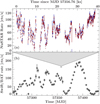 |
Fig. 1. a: light curve of the observation as seen by NuSTAR. Red and blue data points show the NuSTAR light-curve corresponding to FPMA and FPMB. b: Swift/BAT (Krimm et al. 2013) light-curve of Cen X-3 around the observation time, binned to the orbital period of ∼2.08 d. |
In order to investigate the spectrum down to 1 keV we include contemporaneous Swift data (Gehrels et al. 2004) taken taken on 2015 December 10 (ObsID 00081666001) with a total exposure time of 425 s in Photon Counting Mode (PC) and 1522 s in Windowed Timing mode. To mitigate the significant pile up in the PC mode data, we defined the source region as an annulus with inner radius of 8 pixel and outer radius of 30 pixel, and use a 60 pixel circle offset from the source to extract the background. In Windowed Timing mode Swift-XRT has only one dimensional imaging capabilities. For this mode, the central 20 pixels were used as the source region. A region between 80 pixel and 120 pixel away from the source on both sides was used as the background.
In the following spectral analysis, which was performed with ISIS version 1.6.2-41 (Houck & Denicola 2000), we use the NuSTAR data in the energy band between 3.5 keV and 79 keV, while the Swift data were considered in the band from 1.0 keV to 10 keV.
3. Fitting the accretion rate of BWsim
3.1. The accretion column model by Becker & Wolff (2007)
A detailed description of the accretion model BWsim is given by BW07 and Wolff et al. (2016), so we only summarize its key features: The gas entering the cylindrical column from the top is decelerated in an extended radiation-dominated standing shock region and eventually settles on the thermal mound at the bottom of which it reaches a velocity of zero. In this column, the deceleration of the accreted matter leads to the emission of photons. Specifically the following three types of seed photons are considered by BW07: Blackbody radiation from the hot thermal mound4 at the bottom of the accretion column; Bremsstrahlung emitted by the electrons streaming along the magnetic field (free-free emission); and Cyclotron radiation produced by the decay of electrons collisionally excited to the first Landau level5.
As they propagate through the column, these photons then interact with the accreted material. For the radiative transport one needs to account for both bulk and thermal Comptonization of seed photons (i.e., first- and second-order Fermi energization due to collisions with gas deceleration along the z-axis), which leads to a two-dimensional radiative transfer equation. The photon distribution f(z, ϵ) is a function of the height z and the photon energy ϵ and, as given by BW07 (Eq. (15)), the transport equation is given by
![Mathematical equation: $$ \begin{aligned} \frac{\partial f}{\partial t} + { v} \, \frac{\partial f}{\partial z} =&\frac{\mathrm{d}{ v}}{\mathrm{d}z}\,\frac{\epsilon }{3} \, \frac{\partial f}{\partial \epsilon } + \frac{\partial }{\partial z}\left(\frac{c}{3 n_{\rm e} \sigma _\parallel }\,\frac{\partial f}{\partial z}\right)\nonumber \\&- \frac{f}{t_{\rm esc}} + \frac{n_{\rm e} \bar{\sigma } c}{m_{\rm e} c^2} \frac{1}{\epsilon ^2} \frac{\partial }{\partial \epsilon }\left[\epsilon ^4\left(f + k T_{\rm e} \, \frac{\partial f}{\partial \epsilon }\right)\right] + \frac{Q(z,\epsilon )}{\pi r_0^2}, \end{aligned} $$](/articles/aa/full_html/2021/12/aa40582-21/aa40582-21-eq1.gif) (1)
(1)
where z is the distance from the stellar surface along the column axis, v is the inflow velocity, tesc represents the mean time photons spend in the plasma before diffusing through the walls of the column, σ∥ is the electron scattering cross-section parallel to the magnetic field,  is the angle-averaged mean scattering cross-section and Q(z, ϵ) denotes the photon source distribution.
The left-hand side of Eq. (1) describes the time derivative of the photon density in the co-moving reference frame, while the right-hand side accounts for (from left to right) bulk Comptonization inside the radiative shock region, diffusion of photons along vertical column axis, escape of photons though the column walls, thermal Comptonization described by the Kompaneets operator (Kompaneets 1957), and the injection of seed photons into the accretion column.
The escape time tesc, which quantifies the diffusion of photons through the column walls, is only a function of height along the column and is, similar to the scattering cross-sections, already averaged over polarization states and photon energies. However, as indicated by Eq. (18) from BW07, the escape time utilized the perpendicular scattering cross section σ⊥, and is therefore sensitive to the direction of propagation. To make an analytical solution feasible it is necessary to assume a temperature profile that is constant over the accretion column. There have been numerical calculations showing significant temperature variation inside the column (Mushtukov et al. 2015; West et al. 2017). However, one would expect that inverse-Compton ‘thermostat’ to keep the electron temperature roughly constant in the region of the accretion column where Comptonization is strongest, which is the same region that generates most of the observed radiation.
One should also note that resonant scattering is not included in the BW07 model. This is probably reasonable for sources with relatively strong magnetic fields, so that the cyclotron energy is around ∼40 keV or higher, because in this case most of the photon scattering occurs away from the resonance, in the continuum region of the cyclotron cross section (see discussion just before Eq. (6) in BW07).
The escaping spectrum, which is derived from the photon distribution f and trsc using Eq. (69) of BW07, is integrated along the column height to yield the detectable spectrum.
BW07 also showed that the assumption of a velocity profile linear in optical depth, τ, results in a radiation transfer equation that is separable in energy and space, which in turn allows the derivation of a Green’s function which can then be applied to the three seed photon distributions mentioned above. While the resulting computing times are still large compared to phenomenological models, they are small enough that direct comparisons between the model and data are possible. In the resulting model the free parameters are the mass accretion rate, Ṁ, the column radius, r0, the magnetic field strength responsible for the cyclotron seed photons, B0, the electron temperature of the Comptonizing electrons Te, and two so-called similarity parameters6δ and ξ, which describe properties of the accretion flow and of the radiative transfer in the accretion column (see Eqs. (3) and (4) of Wolff et al. 2016). Specifically, ξ is related to the ratio of the accretion and photon escape timescales below the shock
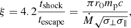 (2)
(2)
where mp is the proton mass, and δ is related to the Compton-y-parameters for bulk motion and thermal Comptonization,
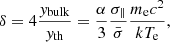 (3)
(3)
where
 (4)
(4)
and where M* and R* are the mass and radius of the NS, σ∥ is the average scattering cross-section perpendicular to the magnetic field, and ybulk and yth are the Compton y-parameters as defined by Rybicki & Lightman (1986). In order to solve Eq. (1) analytically, in addition to the approximate velocity profile, BW07 assume a uniform temperature cylindrical accretion flow in a constant B-field, which is in a steady state and consists of a fully ionized hydrogen plasma. The electron cross-sections are approximate and estimated for electrons propagating parallel or perpendicular to the magnetic field and interacting with photons having the mean photon energy, that is averaged over the photon energy. These assumptions limit the application to strongly magnetized NS at high accretion rates, where radiation pressure plays a dominant role in the deceleration. This should make the model applicable down to luminosities around Lx ∼ 1035 − 36 erg s−1, but an assessment of the validity of the model assumptions is recommended on a case-by-case basis. An overview of the resulting free model parameters is shown in Table 1.
Overview of the free parameters of the accretion column model by Becker & Wolff (2007).
3.2. Iterative approach for energy conservation
A fundamental difficulty of the application of the BW07 model (which is also present in the model of Farinelli et al. 2012) when fitting X-ray spectra is that for many parameter combinations it lacks self-consistency and does not automatically conserve energy. Specifically, there can be a mismatch between the integrated “X-ray luminosity”,
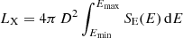 (5)
(5)
and the accretion luminosity
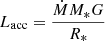 (6)
(6)
as estimated from the loss of potential energy of the accreted material, assuming that all accretion energy is radiated away. In Eqs. (5) and (6) SE(E) is the model-predicted photon flux adjusted to the rest frame of the accretion column7, Emin and Emax are appropriate energy bounds for the integration over the energy E, D is the distance to the source, Ṁ is the mass accretion rate, M* and R* are the NS’s mass and radius, respectively, and G is the gravitational constant. We note that the Ṁ is not just a scaling parameter, but it is also connected to the shape of the emitted spectrum, since, e.g., the cyclotron and bremsstrahlung seed photon generation is a function of density and hence Ṁ, whereas the blackbody seed photon injection only depends on the size and temperature of the polar cap. The mass accretion rate parameter is therefore correlated to some extent with other model parameters determining the spectral shape and cannot be constrained uniquely from the observed flux. Based on the argument of energy conservation, parameter combinations resulting in good description of the spectral shape but with a strong mismatch of the accretion and X-ray luminosity therefore have to be rejected. Since these invalid solutions cannot be avoided a priori, e.g., by choosing appropriate 1D parameter boundaries, other strategies of ensuring consistent parameter solutions during the fitting procedure are required. While such higher dimensional constraints on the parameter space can be accounted for quite directly in fitting algorithms that sample the parameter space (e.g., Markov chain Monte Carlo) by rejecting invalid parameter combinations, typical χ2-minimization algorithms require a certain integrity of the parameter space. Wolff et al. (2016) therefore propose an interactive approach to ensure energy conservation manually when comparing the BW07 model to observations. This approach is typically done by estimating Ṁ from the source spectrum by positing that LX equals Lacc. Holding this Ṁ fixed, the model is then fit to the data, obtaining a new set of best-fit parameters. This fit, however, will generally change the integrated luminosity of the model. The new fit is therefore not consistent with the initial condition of LX = Lacc. One then iterates the fit by adjusting the parameters until equality of both parameters is reached.
In practical terms, to determine a first guess for the accretion rate, the observed spectrum is initially fitted with an empirical model, i.e., some type of power-law with an exponential cut-off (see, e.g., Müller et al. 2013, for a description of the relevant models). One then uses this fit and the known distance to calculate an initial LX, and from Eqs. (5) and (6) then obtains an an initial accretion rate Ṁ8. This estimate is then followed by a first χ2-minimization using a BWsim continuum with Ṁ held fixed at this value. The resulting flux is then used to derive a new value of Ṁ, and this approach is iterated until convergence is reached in Ṁ, i.e., once the relative change in Ṁ becomes smaller than a certain threshold, here 1%. For the joint Swift/NuSTAR data of Cen X-3 this method converges after 3−6 iterations. In practice, this method is a very cumbersome approach that requires significant manual intervention and “baby sitting” of the fits, hindering the application to larger samples of spectral data. Another issue with this iterative approach is that during each minimization step Ṁ is treated as a fixed parameter and is, therefore, not allowed to deviate from the value derived from the model luminosity. This approach neglects the fact that, e.g., the distance to the source is not precisely known, which would result in a systematic shift in the assumed accretion rate.
3.3. Biasing the fit statistics
To avoid the interactive procedure we propose an alternative strategy to address this issue which does not require an iterative approach but rather introduces energy conservation directly into the data modeling. The idea of our technique is to let Ṁ vary during the fit, but to bias the fit statistics in a way that it disfavors values of Ṁ which do not fulfill energy conservation, i.e., for which LX ≠ Lacc. In ISIS, this approach can easily be implemented as one has a direct programmatic access to the fit statistics calculation that allows one to modify its value during the minimization.
For the case of χ2-statistics, the value to be minimized is
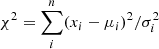 (7)
(7)
where the sum goes over all spectral channels, i, and where xi are the data counts with uncertainties, σi, and μi the counts predicted by the model. We now modify χ2 to rise with increasing difference of the accretion and X-ray luminosities,
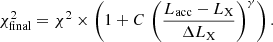 (8)
(8)
Here ΔLX is the uncertainty on the source luminosity introduced by the uncertain distance to the object and other factors such as the lack of knowledge of the emission pattern and accretion column geometry, while C and γ are parameters adjusted in order to optimize the convergence behavior of the χ2-minimization algorithm and to determine the strength of the constraint. Our numerical investigations suggest to set C ∼ 5 and γ ∼ 4, which leads to quick convergence when using a Levenberg-Marquardt method. We found that these numbers worked well for the datasets discussed in this paper. However, they are not guaranteed to be ideal for every dataset, depending on, e.g., the used minimization algorithm and the number of degrees of freedom, adjustments for quicker convergence might become necessary. We settled for this implementation due to its simplicity and its satisfying convergence during fitting (see also Fig. 2). We emphasize that such an approach can be a powerful tool to include additional and potentially complex constraints on the parameter landscape that can not easily be included during model evaluation.
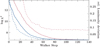 |
Fig. 2. Convergence behavior during the MCMC run with (blue) and without (red) the constraint. The dotted line shows the median of the relative luminosity deviation (|LX−Lacc|/LX) for the walkers of each MCMC step. The solid line indicates, for both runs, the convergence of the regular, unmodified χ2 median of each step. We note that the convergence of the unmodified fit-statistic does not deteriorate while only with our constraint the criterion of energy conservation is quickly reached. |
One possible disadvantage of this approach is that the more complex shape of the χ2 landscape can lead to a tendency of the minimization algorithm to be partly stuck in local minima. Also,  approximates χ2 only close to its minima, where energy is conserved. Consequently this approach should only be used as a tool to find a set of physical best-fit parameters and not to calculate statistical quantities, such as confidence intervals. We validated the reliability of our new approach by reproducing a previous successfully applicable of the model by BW07 to Her X-1. As is described in more detail in the Appendix B, we were able recover previous result by Wolff et al. (2016) with only minor deviations.
4. Application to Cen X-3
Having confirmed our novel approach, we continue to analyze the Cen X-3 observation. In order to allow us to compare the spectral shape with earlier observations, we first fitted the Swift-XRT, NuSTAR-FPMA, and -FPMB spectra with a phenomenological model, i.e., a power-law with an exponential cut-off. Previous studies (e.g., Bissinger né Kühnel et al. 2020; Müller et al. 2013) have shown the significant impact that implementation of the empirical cut-off can have on the cyclotron line parameters, which can lead to unphysically broad and deep lines. In order to probe such a bias, the cut-off was modeled with the two commonly used models: First fdcut, which is defined as
![Mathematical equation: $$ \begin{aligned} F(E) \propto E^{-\Gamma } \frac{1}{1+\exp \left[{\left(E-E_{\mathrm{cut} }\right)/E_{\mathrm{fold} }}\right]} \end{aligned} $$](/articles/aa/full_html/2021/12/aa40582-21/aa40582-21-eq12.gif) (9)
(9)
and second powerlaw × HighEcut, defined as
![Mathematical equation: $$ \begin{aligned} F(E) \propto E^{-\Gamma } {\left\{ \begin{array}{ll} \exp \left[\left(E_{\rm cut}-E\right)/E_{\rm fold}\right]&E \ge E_{\rm c} \\ 1.0&E \le E_{\rm cut} \end{array}\right.} \end{aligned} $$](/articles/aa/full_html/2021/12/aa40582-21/aa40582-21-eq13.gif) (10)
(10)
with the photon index Γ, the folding energy Efold and a cutoff energy Ecut. With a  of 1.32(450) and 1.28(453), respectively, both models describe the spectrum reasonably well. Since HighEcut has a discontinuity at the cut-off energy we smooth this region with an additional absorption component tied to that energy. Incidentally, this gets rid of some residuals caused by calibration issues between 10 keV and 14 keV (see Wolff et al. 2016, and references therein), leading to a slightly lower
  value. As noted previously by, e.g., Burderi et al. (2000), Cen X-3 features very strong fluorescent iron lines between 6 and 7 keV. Most prominent is a neutral Kα line at 6.4 keV, but there are also lines from higher ionization states of He- and H-like iron at 6.7 keV and 6.97 keV, which are also seen in this observation. Additionally a broad iron line feature is necessary to fully account for the iron line complex. A similar feature is also present in the spectrum of Her X-1. While Ebisawa et al. (1996), Naik & Paul (2012) did not require such an feature, a similarly broad iron line is seen in Her X-1. Asami et al. (2014) discussed several possible origins for such a feature, namely unresolved emission lines, Comptonization in an accretion disk corona and Doppler broadening at the inner disk or due to the accretion stream. Similar consideration could be made for Cen X-3 but would exceed the scope of this paper.
The final model includes a calibration constant, Cdet, as well as a partial absorber9, one broad and three narrow Gaussian iron lines10 that have a width smaller than the detector resolution, a broad Gaussian component7, the so-called “10 keV feature”7, and the cyclotron resonance feature around 30 keV, which we model by a multiplicative Gaussian absorption component (gabs11). A similar, preliminary fit to Suzaku data was presented by Marcu et al. (2015) and will be published by Marcu-Cheatham et al. (in prep.). In summary the full model is
 (11)
(11)
where cont stands for the respective empirical continuum model. The parameters values and 90% uncertainties for the corresponding best-fits are given in Table A.1. The residuals for these empirical fits are shown in Fig. 3 (first two residual panels). In a similar work, Tomar et al. (2021) recently performed phenomenological fits to the same NuSTAR data of Cen X-3 as used by us. To describe the continuum they considered a physical fit based on the theory of BW07. As their focus lay, however, on the evolution of the CRSF and not a physical description of the continuum, they choose a smooth high-energy cut-off model, newhcut, which also led to a lower reduced χ2. Due to the different applied models, our ability to compare these results is limited. However, newhcut is a smoothed version of HighEcut and we would therefore expect our results not to deviate by too much. Indeed, Tomar et al. (2021) derive a photon index of 1.21 ± 0.01, close to the value of  we found with our HighEcut model. Overall, the most notable differences might be the lack of a “10-keV” feature in the analysis by Tomar et al. (2021). We consider it likely that the reason for this is the smoothed out transition region of the newhcut compared to the hard break in the HighEcut model. Assuming a fixed “smoothing width” of 5 keV, Tomar et al. (2021) find a cut-off energy, Ecut = 14.14 ± 0.06 keV. This result places the transition region at a similar position and width as our “10-keV” feature. A more detailed comparison would be needed to pin-down the precise differences. Further, the CRSF energy derived from our analysis is consistent with the value of
  keV derived by Tomar et al. (2021), further indicating that the CRSF energy is well constrained by the NuSTAR data.
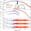 |
Fig. 3. Spectrum of Cen X-3 as seen by NuSTAR and Swift. a: unfolded spectrum and the different components of the BWsim best-fit model. The difference between the unfolded data points and the model is caused by the algorithm used to unfold the data. In black the full spectrum is shown and colored are the different components. b: spectrum fitted with BWsim. Red and orange indicate the data from the two focal plane modules of NuSTAR and shown in dark and light blue is the Swift data in window timing and photon counting mode. c–e: residuals for the FDcut, HighEcut and the BWsim model. |
As a next step, we apply the physical model BWsim to the spectra. The full model is defined as
 (12)
(12)
Since BWsim calculates the emitted radiation in the reference frame of the NS, it is necessary to account for the gravitational redshift, which is done with the zashift component. BWsim alone could not account for the “10-keV” feature and a broad Gaussian had to be included as part of the continuum. Initially the iterative approach was used to fit the described model. The resulting best fit had a reduced χ2 of 1.32 with 601 d.o.f. After the iteration converged Ṁ was fixed to 1.67 × 10¹⁷ g s−1. With the new fitting approach, i.e., including a χ2-penalty (see Eq. (8)) almost identical results were obtained (see Table A.2 for the best-fit parameters utilizing both methods).
To constrain parameter degeneracies, we therefore made use of a Markov-chain Monte Carlo (MCMC) fitting approach, using the ISIS implementation of the MCMC Hammer code (Foreman-Mackey et al. 2013) by M. A. Nowak. For this analysis each MCMC chain was run with ten walkers per free parameter, ignoring the first 60% of the chain to allow the walker distribution to converge. In order to investigate the effect of our constraint we performed three MCMC runs: Once with the accretion rate as an once unconstrained free parameter, once with Ṁ fixed the previously found best-fit value of 1.67 × 10¹⁷ g s−1, and finally with the new constraint applied. For the parameters of the BW07 model, the resulting one- and two-dimensional marginal posterior density distributions are shown in Fig. 5. It is apparent that, without any constraint, only little information about the accretion rate can be gained. Even though the distribution is still well behaved, it is significantly wider than for the constrained fits. Through a strong parameter degeneracy, this wider distribution translates to a large uncertainty in r0. The reason is that in the unconstrained fits, Ṁ can shift away from values that conserve energy, and therefore we also observe a systematic shift in most of the other model parameters.
When applying the constraint, the distribution in Ṁ is collapsed, even though further, smaller parameter degeneracies remain, which are inherent to the BW07 model. When comparing the walker distributions between our constraint and a fixed accretion rate, there are only minor deviations.
To further illustrate these parameter correlations and the effect of our constraint, we color-code a subset of the walkers by the luminosities of their respective model. The result for the most interesting parameters is shown in Fig. A.1. The continuum parameter not only clearly correlate with each other, but also with the model luminosity, so that, e.g., a larger column radius also leads to a higher luminosity. Further emphasized by the color coding is the influence of the continuum parameter on the 10 keV feature and the CRSF, as both show a clear color gradient marking high luminosities and consequently, e.g., high values of r0. This positive correlation between r0 and the model luminosity might be surprising, as an increase in r0, with otherwise constant parameters, reduces the luminosity of the BW07 model. However, to order to still describe the data other continuum parameters have to change as well, more than compensating the luminosity decrease that would result from an increase in r0 alone.
The resulting “best-fit” parameters of the MCMC analysis are shown in Table 2 as the median value and the 90% confidence intervals derived as 90% quantiles of the run with a fixed accretion rate. Figure 4 demonstrates how exactly the model changes along the parameter degeneracy. With increasing r0 the Comptonized bremsstrahlung component in the model decreases in dominance, while the thermal and cyclotron components, as well as the 10-keV feature, increase in strength. These changes compensate for the flux lost in the decreased Comptonization component. These changes in the continuum also drive the correlation between the strength and width of the 10-keV feature, as these adjustments are required for a satisfactory fit, since the feature is used to “fill in” the lost flux in the 10 keV band. Similarly, by investigating the correlation between CRSF width and the BW parameters we see how the modeled cyclotron line changes in width with the continuum, while its centroid energy is comparably well constrained. As expected and seen in the ratio plot, the spectral fluxes differ primarily at high or low energies, where data are sparse or unavailable. These changes in luminosity at the edges of the available energy range may also lead to the discussed violation of energy conservation when Ṁ is just fixed during χ2 minimization.
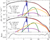 |
Fig. 4. Similar to the upper panel in Fig. 3 the two plots of the unfolded spectrum display individual model components and demonstrate the spectral change along the parameter correlation. a: model components for a small column radius. b: model components for a larger column radius. c: ratio between the high and low radius model. |
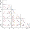 |
Fig. 5. One- and two-dimensional marginal posterior density distributions derived from the MCMC walker distribution. In red the distributions for a free accretion rate, in blue the distribution under the influence of the constraint and in yellow with Ṁ fixed to the value found with the help of the constraint. The solid lines in the two-dimensional subplots denote the 1-sigma contours of the walker distribution. |
Results of the MCMC analysis.
5. Discussion
In this paper we have applied several different modeling approaches to the NuSTAR and Swift spectra of Cen X-3. Our phenomenological approach confirms the stable spectral parameters of Cen X-3 over the last decade (Suchy et al. 2008; Naik & Paul 2012, and references therein).
In order to apply BWsim in any meaningful way, one has to constrain its parameter Ṁ. To this end we require LX and Lacc to be equal, which, however, is only the case if the released energy is emitted isotropically. This has been shown to be generally not the case (see, e.g., Fig. 3.16 of Falkner 2018). Unfortunately, the value obtained with this constraint is still the best guess, as the information on the geometry of the system, which is necessary to improve this assumption, such as the inclination of the NS’s rotational axis or the emissivity pattern of the accretion columns, is lacking.
In the model by BW07, the geometry of the accretion column is fully described by the column radius, r0. Interestingly our best-fit for Cen X-3 shows a column radius of just 63 m. This is just a fraction of the 730 m estimated by BW07 in a “fit by eye” of the model to earlier data of Cen X-3. While these authors used earlier observations with a ∼3.5 times higher unabsorbed luminosity (Burderi et al. 2000), the varying luminosity can only account for ∼20% of the variation of the column radius according to Eq. (112) in BW07.
Another application of BW07 to Cen X-3 has been presented by Gottlieb et al. (2016) and will be published by Marcu-Cheatham et al. (in prep.). These fits yield a column radius of around 65 m, in line with the results presented here. The large deviation between the column radius presented here and that found by BW07 may partially originate from the larger distance to Cen X-3 of 8 kpc used in previous studies, while we used the newer estimate of 5.7 kpc by Thompson & Rothschild (2009). Consequently this leads to a higher inferred luminosity and accretion rate, and, as shown in the parameter correlations, a higher Ṁ will require a larger r0 to model the same spectrum. As also mentioned previously, during that observation the source had about twice the 1−80 keV unabsorbed luminosity (4.0 × 1037 erg s−1) than in our observation (2.1 × 1037 erg s−1). One has to be careful when comparing observations at different unabsorbed luminosities as the clumpy accretion stream does lead to varying accretion rates which affect the structure of the accretion column.
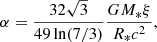
Following Davidson & Ostriker (1973), assuming a dipole geometry one can estimate the column radius from the accretion rate and the magnetic field strength,
 (13)
(13)
where R* is the radius of the NS and Rm is radius where the plasma couples to the magnetic field lines. This radius can be expressed in terms of the classical Alfvén radius RA as Rm = kRA with
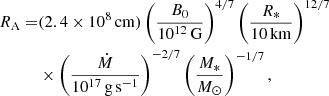 (14)
(14)
where B0 is the magnetic field strength, Ṁ is the accretion rate, and M* is the mass of the NS. Estimates for the parameter k typically vary between 0.5 and 1 (Ghosh & Lamb 1979; Wang 1996; Romanova et al. 2008). Using this range and the parameters of Cen X-3 yields Rm of 2000−4000 km and r0 of 500 − 700 m, far wider than our best-fit would suggest, but in good agreement with the results obtained by BW07 for this source.
There are many assumptions that go into the theory of BW07 that could significantly influence the estimated column geometry, specifically its radius. One assumption would be the presence of a more complex accretion structure. For misaligned magnetic and accretion disk axes one would expect a hollow accretion column or an accretion curtain (Basko & Sunyaev 1976; West et al. 2017; Campbell 2012; Perna et al. 2006). Such a geometry would lead to a much thinner accretion stream than the solid column that is assumed in the model of BW07. It is reasonable to believe that such a thin, elongated stream would produce a spectrum that is best approximated by a thin accretion column within BWsim, as both geometries would have a similar effects on parameters such as the escape time of photons inside the column. A very similar model of a hollow accretion column was applied to Cen X-3 by West et al. (2017), who derived an outer column radius of ∼750 m, in much better agreement with the value derived from Eq. (14), and a width for the column wall of ∼100 m, which is in the order of our column radius.
Another mechanism that can have a significant effect on the spectrum and is not yet included in the BW07 is the interception of radiation from the accretion column by the NS surface and its subsequent reprocessing in the NS atmosphere. This “reflection” model was proposed by Poutanen et al. (2013) as a possible explanation for the origination of cyclotron lines in spectra of accreting X-ray pulsars. Lutovinov et al. (2015) have successfully applied the reflection model to the observational data of the X-ray transient V 0332+53 to describe the variability of the cyclotron line parameters. Postnov et al. (2015) show that reflection from the neutron star surface can also lead to significant hardening of the spectrum in the case of a filled accretion column. In order to estimate the importance of this effect, one needs to know the spectrum of radiation emitted at different heights of the column, as well as the angular distribution of the emission. This information is currently not included in the BW07 model, and therefore modeling the reflection from the NS surface is outside the scope of this work. We note that in the case of a hollow accretion column, the stopping and main emission occur much closer to the surface and the reflection has no noticeable effect on the continuum (Postnov et al. 2015).
Finally, we address the validity of some of the fitted CRSF parameters. In agreement with past measurements (see, e.g., Fig. 5 of Tomar et al. 2021, for an overview of past CRSF measurements of Cen X-3), the CRSF was found in all fits at ∼30 keV and with a width varying between 3.8 and 7.9 keV. The expected width of the cyclotron line can be estimated by calculating the Doppler shift due to thermal broadening (Schwarm et al. 2017; Meszaros & Nagel 1985),
 (15)
(15)
where E is the cyclotron energy, θ is the viewing angle relative to the magnetic moment, and T is the electron temperature. Using the electron temperature derived from the physical fits, we find ΔE ∼ 6.5 keV|cos θ|. Although the average viewing angle is hard to constrain, this estimate indicates that, at least for our physical fits, the CRSF seems to be slightly wider than expected from thermal broadening, This could again be a result of the choice of continuum, as we have seen that this can significantly influence the shape of the cyclotron line. Alternatively, such additional broadening might also be induced by varying magnetic field strength along the height of the column and/or by a varying temperature profile within the column (West et al. 2017; Falkner 2018). Taking all these assumptions into account, the electron temperature falls well inside the expected range of values.
As a quick check of some of the model assumptions, we can calculate the integration height zmax and the height of the sonic point zsp according to Eqs. (80) and (31) of BW07, as most of the emission is expected to occur below the sonic point. One finds zmax = 5.5 km and zsp = 2.8 km. Importantly the sonic shock lies within the integration region, as it is supposed to be. Further, following Wolff et al. (2016), the “blooming fraction” at the sonic point can be obtained, ((R* + zsp)/R*)3 = 2.1, which clearly exceeds unity, hinting at a deviation from a simple cylindrical geometry.
Similarly, assuming a dipole magnetic field, we can calculate the magnetic field strength at the sonic point to be 1.6 B12, which also indicates that the assumption of a constant magnetic field might introduce systematic errors. However, to which degree this actually affects our results is hard to specify as the emission intensity along the column height is not directly accessible.
Finally, from the similarity parameters ξ and δ, it is possible to derive the average electron scattering cross-section  and the cross-section parallel to the magnetic field σ∥ = 3.12 × 10⁻⁵σT, while the cross-section perpendicular to the magnetic field is frozen to the Thomson cross-section σT. These are ordered as one would expect
  and are generally in the order of, but some-what lower than, the cross-section derived by BW07.
In summary, while the BW07 model describes the physical processes of the formation of the radiation well, its assumption of a filled cylindrical accretion column of constant radius is likely to introduce systematic errors in the geometry parameters when comparing the model with data. Further development of the model toward a more realistic column structure is therefore needed. We emphasize that despite these simplifications, besides the implementation by Farinelli et al. (2012), the model is still the only physics-based model for accretion column emission applicable to fitting observational data and that the major conclusions drawn from fits of the BW07 model, e.g., the dominance of bulk motion Comptonization or bremsstrahlung emission on the observed spectra, will be largely unaffected by the simplified assumptions for the accretion geometry.
6. Conclusions
In this paper we presented a detailed spectral analysis of combined NuSTAR and Swift spectra of Cen X-3. To simplify application of the physical column model by BW07 to the spectrum of an accreting pulsar, a new approach of fitting was introduced. By biasing the value of χ2 toward physically consistent parameters, it was possible to apply the physical model derived by BW07 without having to assure energy conservation in any other, external way. This approach allows one to explore non standard parameter spaces with efficient χ2-minimization algorithms alternatively to more computationally expensive sampling methods such as MCMC. In many cases, this will considerably simplify the application of the BW07 on observational data but this is also generally applicable to complex spectral models where certain parameter combinations may lead to the violation of model assumptions. With this new approach previous fits to the spectrum of Her X-1 were reproduced and the spectrum of Cen X-3 could be fitted with similar quality as conventional phenomenological models. The familiar features which have been seen in previous studies were found in our analysis as well, e.g., the prominent iron lines, the CRSF at ∼30 keV and a partially absorbed power-law continuum. The parameters of BWsim describing the accretion column suggest a thin or possibly a hollow accretion column or curtain.
We note that the top of the thermal mound is not the same as the NS surface. Therefore matter enters the mound with a certain inflow speed heating the mound to a temperature given by Eq. (93) in BW07.
These seed photons are treated by the model as simply monochromatic without intrinsic line broadening. The strong broadening due to thermal and bulk Componization that the seed photons experience subsequently after their injection would likely wash out the intrinsic broadening of the cyclotron seed photon. Hence the neglect of the intrinsic broadening is probably reasonable.
The alternative parameterization of the model, BWphys, uses the parallel and average scattering cross sections, σ∥ and  , instead of the similarity parameters ξ and δ.
In order to calculate the flux close to the NS surface, where the spectrum emerges, the red-shift of z = 0.3, which is otherwise applied, is set to 0, as well as the column density of both the partial and complete absorption model.
This assumes the released energy is emitted isotropically. We address this assumption in Sect. 5.
Acknowledgments
This work has been funded in part by the Bundesministerium für Wirtschaft und Technologie through Deutsches Zentrum für Luft- und Raumfahrt grants 50 OR 1909. This work used data from the NuSTAR mission, a project led by the California Institute of Technology, managed by the Jet Propulsion Laboratory, and funded by the National Aeronautics and Space Administration. The material is based upon work supported by NASA under award number 80GSFC21M0002. ESL acknowledges support by Deutsche Forschungsgemeinschaft grant WI1860/11-1 and RFBR grant 18-502-12025. This research also made use of the NuSTAR Data Analysis Software (NuSTARDAS) jointly developed by the ASI Science Data Center (ASDC, Italy) and the California Institute of Technology (USA), as well as data from the Swift satellite, a NASA mission managed by the Goddard Space Flight Center. MTW is supported by the NASA Astrophysics Explorers Program and the NuSTAR Guest Investigator Program. This research also has made use of a collection of ISIS functions (ISISscripts) provided by ECAP/Remeis observatory and MIT (http://www.sternwarte.uni-erlangen.de/isis/). Finally, we acknowledge the helpful advice concerning readability and the general support by Victoria Grinberg.
References
- Arnaud, K., Borkowski, K. J., & Harrington, J. P. 1996, ApJ, 462, L75 [NASA ADS] [Google Scholar]
- Asami, F., Enoto, T., Iwakiri, W., et al. 2014, PASJ, 66, 44 [NASA ADS] [CrossRef] [Google Scholar]
- Ash, T. D. C., Reynolds, A. P., Roche, P., et al. 1999, MNRAS, 307, 357 [NASA ADS] [CrossRef] [Google Scholar]
- Basko, M. M., & Sunyaev, R. A. 1976, MNRAS, 175, 395 [Google Scholar]
- Becker, P. A., & Wolff, M. T. 2007, ApJ, 654, 435 [NASA ADS] [CrossRef] [Google Scholar]
- Becker, P. A., Klochkov, D., Schönherr, G., et al. 2012, A&A, 544, A123 [NASA ADS] [CrossRef] [EDP Sciences] [Google Scholar]
- Bissinger né Kühnel, M., Kreykenbohm, I., Ferrigno, C., et al. 2020, A&A, 634, A99 [NASA ADS] [CrossRef] [EDP Sciences] [Google Scholar]
- Burderi, L., Di Salvo, T., Robba, N. R., La Barbera, A., & Guainazzi, M. 2000, ApJ, 530, 429 [NASA ADS] [CrossRef] [Google Scholar]
- Campbell, C. G. 2012, MNRAS, 420, 1034 [NASA ADS] [CrossRef] [Google Scholar]
- Davidson, K., & Ostriker, J. P. 1973, ApJ, 179, 585 [NASA ADS] [CrossRef] [Google Scholar]
- Ebisawa, K., Day, C. S. R., Kallman, T. R., et al. 1996, PASJ, 48, 425 [NASA ADS] [Google Scholar]
- Falkner, S. 2018, PhD Thesis, FAU Erlangen [Google Scholar]
- Farinelli, R., Ceccobello, C., Romano, P., & Titarchuk, L. 2012, A&A, 538, A67 [NASA ADS] [CrossRef] [EDP Sciences] [Google Scholar]
- Ferrigno, C., Becker, P. A., Segreto, A., Mineo, T., & Santangelo, A. 2009, A&A, 498, 825 [NASA ADS] [CrossRef] [EDP Sciences] [Google Scholar]
- Foreman-Mackey, D., Hogg, D. W., Lang, D., & Goodman, J. 2013, PASP, 125, 306 [Google Scholar]
- Gehrels, N., Chincarini, G., Giommi, P., et al. 2004, ApJ, 611, 1005 [Google Scholar]
- Ghosh, P., & Lamb, F. K. 1979, ApJ, 232, 259 [Google Scholar]
- Giacconi, R., Gursky, H., Kellogg, E., Schreier, E., & Tananbaum, H. 1971, ApJ, 167, L67 [NASA ADS] [CrossRef] [Google Scholar]
- Gornostaev, M. I. 2021, MNRAS, 501, 564 [Google Scholar]
- Gottlieb, A., Pottschmidt, K., Marcu, D., et al. 2016, AAS/High Energy Astrophysics Division, 15, 120.09 [NASA ADS] [Google Scholar]
- Harrison, F. A., Craig, W. W., Christensen, F. E., et al. 2013, ApJ, 770, 103 [Google Scholar]
- Houck, J. C., & Denicola, L. A. 2000, in Astronomical Data Analysis Software and Systems IX, eds. N. Manset, C. Veillet, & D. Crabtree, ASP Conf. Ser., 216, 591 [Google Scholar]
- Kawashima, T., & Ohsuga, K. 2020, PASJ, 72, 15 [NASA ADS] [CrossRef] [Google Scholar]
- Kompaneets, A. S. 1957, Sov. J. Exp. Theor. Phys., 4, 730 [Google Scholar]
- Krimm, H. A., Holland, S. T., Corbet, R. H. D., et al. 2013, ApJS, 209, 14 [NASA ADS] [CrossRef] [Google Scholar]
- Langer, S. H., & Rappaport, S. 1982, ApJ, 257, 733 [NASA ADS] [CrossRef] [Google Scholar]
- Lutovinov, A. A., Tsygankov, S. S., Suleimanov, V. F., et al. 2015, MNRAS, 448, 2175 [NASA ADS] [CrossRef] [Google Scholar]
- Marcu, D. M., Pottschmidt, K., Gottlieb, A. M., et al. 2015, ArXiv e-prints [arXiv:1502.03437] [Google Scholar]
- Marcu-Cheatham, D. M., Pottschmidt, K., Wolff, M. T., & Gottlieb, A. M. 2022, MNRAS, submitted [Google Scholar]
- Meszaros, P., & Nagel, W. 1985, ApJ, 298, 147 [NASA ADS] [CrossRef] [Google Scholar]
- Müller, S., Ferrigno, C., Kühnel, M., et al. 2013, A&A, 551, A6 [NASA ADS] [CrossRef] [EDP Sciences] [Google Scholar]
- Mushtukov, A. A., Suleimanov, V. F., Tsygankov, S. S., & Poutanen, J. 2015, MNRAS, 447, 1847 [NASA ADS] [CrossRef] [Google Scholar]
- Nagase, F., Corbet, R. H. D., Day, C. S. R., et al. 1992, ApJ, 396, 147 [NASA ADS] [CrossRef] [Google Scholar]
- Naik, S., & Paul, B. 2012, Bull. Astron. Soc. India, 40, 503 [NASA ADS] [Google Scholar]
- Paul, B., Raichur, H., & Mukherjee, U. 2005, A&A, 442, L15 [NASA ADS] [CrossRef] [EDP Sciences] [Google Scholar]
- Perna, R., Bozzo, E., & Stella, L. 2006, ApJ, 639, 363 [NASA ADS] [CrossRef] [Google Scholar]
- Postnov, K. A., Gornostaev, M. I., Klochkov, D., et al. 2015, MNRAS, 452, 1601 [Google Scholar]
- Poutanen, J., Mushtukov, A. A., Suleimanov, V. F., et al. 2013, ApJ, 777, 115 [NASA ADS] [CrossRef] [Google Scholar]
- Romanova, M. M., Kulkarni, A. K., & Lovelace, R. V. E. 2008, ApJ, 673, L171 [Google Scholar]
- Rybicki, G. B., & Lightman, A. P. 1986, Radiative Processes in Astrophysics (New York: Wiley) [Google Scholar]
- Santangelo, A., del Sordo, S., Segreto, A., et al. 1998, A&A, 340, L55 [NASA ADS] [Google Scholar]
- Schreier, E., Levinson, R., Gursky, H., et al. 1972, ApJ, 172, L79 [NASA ADS] [CrossRef] [Google Scholar]
- Schwarm, F. W., Schönherr, G., Falkner, S., et al. 2017, A&A, 597, A3 [NASA ADS] [CrossRef] [EDP Sciences] [Google Scholar]
- Shapiro, S. L., & Salpeter, E. E. 1975, ApJ, 198, 671 [Google Scholar]
- Staubert, R., Trümper, J., Kendziorra, E., et al. 2019, A&A, 622, A61 [NASA ADS] [CrossRef] [EDP Sciences] [Google Scholar]
- Suchy, S., Pottschmidt, K., Wilms, J., et al. 2008, ApJ, 675, 1487 [NASA ADS] [CrossRef] [Google Scholar]
- Thompson, T. W. J., & Rothschild, R. E. 2009, ApJ, 691, 1744 [NASA ADS] [CrossRef] [Google Scholar]
- Tjemkes, S. A., Zuiderwijk, E. J., & van Paradijs, J. 1986, A&A, 154, 77 [NASA ADS] [Google Scholar]
- Tomar, G., Pradhan, P., & Paul, B. 2021, MNRAS, 500, 3454 [Google Scholar]
- Truemper, J., Pietsch, W., Reppin, C., et al. 1978, ApJ, 219, L105 [CrossRef] [Google Scholar]
- Wang, Y. M. 1996, ApJ, 465, L111 [Google Scholar]
- Wang, Y. M., & Frank, J. 1981, A&A, 93, 255 [Google Scholar]
- West, B. F., Wolfram, K. D., & Becker, P. A. 2017, ApJ, 835, 130 [NASA ADS] [CrossRef] [Google Scholar]
- Wolff, M. T., Becker, P. A., Gottlieb, A. M., et al. 2016, ApJ, 831, 194 [Google Scholar]
- Wolff, M., Becker, P. A., Coley, J., et al. 2019, BAAS, 51, 386 [NASA ADS] [Google Scholar]
Appendix A: Fit parameters
Best-fit parameters for empirical models applied to the Cen X-3 observation.
Best-fit parameters for BWsim model applied to the Cen X-3 observation.
 |
Fig. A.1. One- and two-dimensional marginal posterior density distributions derived from the MCMC walker distribution. For this run Ṁ was fixed. The under-laying gray contour shows the walker distribution of the converged chain. A random subset of walkers was picked out and color-coded by luminosity, with walkers corresponding to a bright model colored in red and less bright Walkers colored in blue. †: Multiplied by 100. |
Appendix B: Proof of concept: Her X-1
To validate our new approach, we applied it to archival data of Her X-1 which was already successfully modeled by Wolff et al. (2016) with their iterative approach, before then turning to the analysis of NuSTAR and Swift data of Cen X-3.
Her X-1 is an intermediate-mass X-ray pulsar and the first source in which a cyclotron line was observed (Truemper et al. 1978). It was observed by NuSTAR (ObsID 30002006005) on 2012 September 22, when it reached a luminosity of ∼4.9 × 1037 erg s−1, putting Her X-1 above or close to the super-critical luminosity according to (Becker et al. 2012), As Wolff et al. (2016) have estimated a critical luminosity for Her X-1 of Lcrit ∼ 7.3 × 1036 erg s−1.
Wolff et al. (2016) excluded the region between 10 keV and 14.4 keV due to uncertainties in the calibration. For consistency, the same was done in this analysis. The comparison between the best fit, found with the new approach and the classical approach, shown in Fig. B.1 and Table B.1, illustrates their convergence to equivalent fits. Any remaining deviations are consistent with being due to the slightly different calibration used for the data extraction and the fact that Wolff et al. (2016) allowed the accretion rate to deviate by 30% from complete energy conservation.
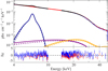 |
Fig. B.1. Proof of concept: Comparison between the best fit to the spectrum of Her X-1, obtained with the new fitting approach (solid lines in the upper panel and red residuals in the bottom panel) and the fit performed by Wolff et al. (2016) (dashed lines in the upper panel and blue residuals in the bottom panel). The red component corresponds to Comptonized bremsstrahlung, the orange one to Comptonized cyclotron emission, the violet one to the Comptonized blackbody emission, and the blue one to the iron line complex. The corresponding parameter values are shown in Tab. B.1. |
Proof of concept of our novel fitting method: Comparison of our best-fit BWsim parameters for Her X-1 and the ones found by Wolff et al. (2016). As discussed in Sect. 3, for the new approach the “uncertainties” have lost their strict meaning of confidence interval. They illustrate, however, that close to the chi-square minimum the distortion of the confidence intervals is small. The plot of the two models and the corresponding residuals are shown in Fig. B.1.
All Tables
Overview of the free parameters of the accretion column model by Becker & Wolff (2007).
Proof of concept of our novel fitting method: Comparison of our best-fit BWsim parameters for Her X-1 and the ones found by Wolff et al. (2016). As discussed in Sect. 3, for the new approach the “uncertainties” have lost their strict meaning of confidence interval. They illustrate, however, that close to the chi-square minimum the distortion of the confidence intervals is small. The plot of the two models and the corresponding residuals are shown in Fig. B.1.
All Figures
|
Fig. 1. a: light curve of the observation as seen by NuSTAR. Red and blue data points show the NuSTAR light-curve corresponding to FPMA and FPMB. b: Swift/BAT (Krimm et al. 2013) light-curve of Cen X-3 around the observation time, binned to the orbital period of ∼2.08 d. |
| In the text | |
|
Fig. 2. Convergence behavior during the MCMC run with (blue) and without (red) the constraint. The dotted line shows the median of the relative luminosity deviation (|LX−Lacc|/LX) for the walkers of each MCMC step. The solid line indicates, for both runs, the convergence of the regular, unmodified χ2 median of each step. We note that the convergence of the unmodified fit-statistic does not deteriorate while only with our constraint the criterion of energy conservation is quickly reached. |
| In the text | |
|
Fig. 3. Spectrum of Cen X-3 as seen by NuSTAR and Swift. a: unfolded spectrum and the different components of the BWsim best-fit model. The difference between the unfolded data points and the model is caused by the algorithm used to unfold the data. In black the full spectrum is shown and colored are the different components. b: spectrum fitted with BWsim. Red and orange indicate the data from the two focal plane modules of NuSTAR and shown in dark and light blue is the Swift data in window timing and photon counting mode. c–e: residuals for the FDcut, HighEcut and the BWsim model. |
| In the text | |
|
Fig. 4. Similar to the upper panel in Fig. 3 the two plots of the unfolded spectrum display individual model components and demonstrate the spectral change along the parameter correlation. a: model components for a small column radius. b: model components for a larger column radius. c: ratio between the high and low radius model. |
| In the text | |
|
Fig. 5. One- and two-dimensional marginal posterior density distributions derived from the MCMC walker distribution. In red the distributions for a free accretion rate, in blue the distribution under the influence of the constraint and in yellow with Ṁ fixed to the value found with the help of the constraint. The solid lines in the two-dimensional subplots denote the 1-sigma contours of the walker distribution. |
| In the text | |
|
Fig. A.1. One- and two-dimensional marginal posterior density distributions derived from the MCMC walker distribution. For this run Ṁ was fixed. The under-laying gray contour shows the walker distribution of the converged chain. A random subset of walkers was picked out and color-coded by luminosity, with walkers corresponding to a bright model colored in red and less bright Walkers colored in blue. †: Multiplied by 100. |
| In the text | |
|
Fig. B.1. Proof of concept: Comparison between the best fit to the spectrum of Her X-1, obtained with the new fitting approach (solid lines in the upper panel and red residuals in the bottom panel) and the fit performed by Wolff et al. (2016) (dashed lines in the upper panel and blue residuals in the bottom panel). The red component corresponds to Comptonized bremsstrahlung, the orange one to Comptonized cyclotron emission, the violet one to the Comptonized blackbody emission, and the blue one to the iron line complex. The corresponding parameter values are shown in Tab. B.1. |
| In the text | |
Current usage metrics show cumulative count of Article Views (full-text article views including HTML views, PDF and ePub downloads, according to the available data) and Abstracts Views on Vision4Press platform.
Data correspond to usage on the plateform after 2015. The current usage metrics is available 48-96 hours after online publication and is updated daily on week days.
Initial download of the metrics may take a while.