| Issue |
A&A
Volume 655, November 2021
|
|
|---|---|---|
| Article Number | A42 | |
| Number of page(s) | 17 | |
| Section | Extragalactic astronomy | |
| DOI | https://doi.org/10.1051/0004-6361/202141835 | |
| Published online | 11 November 2021 | |
Molecular gas budget and characterization of intermediate-mass star-forming galaxies at z ≈ 2–3
1
Núcleo de Astronomía de la Facultad de Ingeniería y Ciencias, Universidad Diego Portales, Av. Ejército Libertador 441, Santiago, Chile
e-mail: This email address is being protected from spambots. You need JavaScript enabled to view it.
2
Las Campanas Observatory, Carnegie Institution of Washington, Casilla 601, La Serena, Chile
3
Instituto de Astrofísica, Facultad de Física, Pontificia Universidad Católica de Chile, Av. Vicuña Mackenna 4860, 782-0436 Macul, Santiago, Chile
4
Departamento de Astronomía, Universidad de Chile, Casilla 36-D, Santiago, Chile
5
Instituto de Física, Pontificia Universidad Católica de Valparaíso, Casilla 4059, Valparaíso, Chile
6
Department of Astronomy, University of Michigan, 1085 South University Avenue, Ann Arbor, MI 48109, USA
7
Institute of Theoretical Astrophysics, University of Oslo, PO Box 1029 Blindern, 0315 Oslo, Norway
8
Department of Physics, University of Cincinnati, Cincinnati, OH 45221, USA
9
European Southern Observatory, Alonso de Córdova 3107, Vitacura, Casilla, 19001 Santiago, Chile
10
Observational Cosmology Lab, NASA Goddard Space Flight Center, Code 665, 8800 Greenbelt Rd, Greenbelt, MD 20771, USA
11
Department of Astronomy & Astrophysics, The University of Chicago, 5640 S. Ellis Avenue, Chicago, IL 60637, USA
Received:
20
July
2021
Accepted:
20
August
2021
Abstract
Star-forming galaxies (SFGs) with stellar masses below 1010 M⊙ make up the bulk of the galaxy population at z > 2. The properties of the cold gas in these galaxies can only be probed in very deep observations or by targeting strongly lensed galaxies. Here we report the results of a pilot survey using the Atacama Compact Array of molecular gas in the most strongly magnified galaxies selected as giant arcs in optical data. The selection in rest-frame ultraviolet (UV) wavelengths ensures that sources are regular SFGs, without a priori indications of intense dusty starburst activity. We conducted Band 4 and Band 7 observations to detect mid-J CO, [C I] and thermal continuum as molecular gas tracers from four strongly lensed systems at z ≈ 2 − 3: our targets are SGAS J1226651.3+215220 (A and B), SGAS J003341.5+024217 and the Sunburst Arc. The measured molecular mass was then projected onto the source plane with detailed lens models developed from high resolution Hubble Space Telescope observations. Multiwavelength photometry was then used to obtain the intrinsic stellar mass and star formation rate via spectral energy distribution modeling. In only one of the sources are the three tracers robustly detected, while in the others they are either undetected or detected in continuum only. The implied molecular gass masses range from 4 × 10⁹ M⊙ in the detected source to an upper limit of ≲109 M⊙ in the most magnified source. The inferred gas fraction and gas depletion timescale are found to lie approximately 0.5–1.0 dex below the established scaling relations based on previous studies of unlensed massive galaxies, but in relative agreement with existing literature about UV-bright lensed galaxies at these high redshifts. Our results indicate that the cold gas content of intermediate to low mass galaxies should not be extrapolated from the trends seen in more massive high-z galaxies. The apparent gas deficit is robust against biases in the stellar mass or star formation rate. However, we find that in this mass-metallicity range, the molecular gas mass measurements are severely limited by uncertainties in the current tracer-to-gas calibrations.
Key words: galaxies: high-redshift / galaxies: star formation / gravitational lensing: strong / galaxies: ISM / galaxies: evolution / submillimeter: galaxies
© ESO 2021
1. Introduction
New stars are born from giant, cold molecular gas clouds in dusty environments within the interstellar medium (ISM) of star-forming galaxies (SFGs, Bolatto et al. 2008; Kennicutt & Evans 2012), although the detailed physical mechanisms by which galaxies acquire gas and then convert it into stars are still poorly understood (e.g., McKee & Ostriker 2007). However, theoretical and observational efforts in the past decades have contributed to link the evolution of galactic-scale parameters of star formation (e.g., star formation rate, SFR; stellar mass, Mstars; gas depletion timescale, tdep = Mmol/SFR; etc.) with the abundance and physical conditions of the cold ISM from the Local Universe up to redshift z ∼ 4 (see the recent reviews by Hodge & da Cunha 2020; Tacconi et al. 2020; Förster Schreiber & Wuyts 2020).
The advent of large samples of massive SFGs with targeted dust continuum and/or CO line observations (the two most common molecular gas tracers at high redshift) revealed a number of key trends: a tight correlation between the gas fraction (Mmol/Mstars) and the specific star formation rate (sSFR ≡ SFR/Mstars), a decrease in tdep with redshift, and an increase in the gas fraction with redshift (e.g., Scoville et al. 2017; Tacconi et al. 2018). These results imply that galaxies with higher levels of star formation also have larger molecular gas reservoirs, and that these reservoirs were on average larger in the first gigayears of the universe. The current explanation is that the ability of a galaxy to form stars is regulated by a feedback loop between the cosmological accretion of gas and the return of that gas to the ambient via galactic outflows, a picture that is often refered to as the “equilibrium model” (Davé et al. 2012; Lilly et al. 2013; Walter et al. 2020). Furthermore, deep blind (ASPECS, Decarli et al. 2019, 2020) and archival (A3COSMOS, Liu et al. 2019) surveys conducted with the Atacama Large Millimeter/Submillimeter Array (ALMA) confirm that the cosmic molecular gas density follows roughly the same evolution as the cosmic star formation density, that is with a global maximum occurring around z ≈ 2 (e.g., Madau & Dickinson 2014). However, at z ≳ 1 this picture is necessarily incomplete, since the current statistical samples are limited to the highest-mass systems (1010 M⊙ ≤ Mstars ≤ 1011.5 M⊙) despite lower mass galaxies being more numerous. Unfortunately, directly probing the gas budget of the < 1010 M⊙ galaxies at z ∼ 2 is still a major observational challenge, even with the exquisite sensitivity of ALMA, and has so far been achieved only through stacking techniques (Inami et al. 2020). Low-mass galaxies tend to have a low oxygen abundance (hereafter metallicity) as expected from the mass-metallicity relation (MZR; e.g., Tremonti et al. 2004). This makes the detection of dust and CO even more difficult, since dust is less abundant in low-metallicity environments, favoring the photodissociation of CO molecules (Leroy et al. 2011; Genzel et al. 2012; Bolatto et al. 2013).
A popular alternative for exploring the low-mass regime at high-redshift is to take advantage of strong gravitational lensing. This phenomenon occurs when a distant galaxy is closely aligned along the line of sight with a foreground massive galaxy or cluster of galaxies. The space-time deflection induced by the intervening mass – the lens – produces distorted, magnified, and in some cases, multiple images of the background galaxy projected in the sky, often forming rings or giant arcs. The lensed images appear brighter than they would in the absence of this effect, providing a boost in intrinsic flux limit, that is, at a given instrumental sensitivity, lensing enables the detection of intrinsically fainter sources. Since the lensing effect is stronger toward massive galaxy clusters, the brightest giant arcs are typically found near their cores. Thus, targeting cluster-lensed galaxies became a common strategy for pushing molecular gas studies to fainter and higher redshift galaxies, which provides reliable results if a good model of the lens deflection is available (e.g., Smail et al. 1997; Baker et al. 2004; Danielson et al. 2011; Saintonge et al. 2013; Sharon et al. 2013; Dessauges-Zavadsky et al. 2015; Spingola et al. 2020).
Although giant arcs are rare, directed searches in wide field optical imaging surveys have successfully identified several dozens to this date (Hennawi et al. 2008; Kubo et al. 2010; Stark et al. 2013; Khullar et al. 2021). This number is expected to grow substantially with upcoming surveys such as the Rubin Observatory Legacy Survey of Space and Time (LSST; Ivezić et al. 2019), the Euclid mission (Laureijs et al. 2011), or the Roman Space Telescope (Spergel et al. 2015). For example, Euclid is expected to detect ∼2000 giant arcs in galaxy clusters with a contrast of at least 3σ above the background (Boldrin et al. 2012). The detection of lensed systems in broadband rest-frame UV imaging ensures that the sources are not heavily dust-obscured and can be selected as SFGs by their photometric colors. In contrast to the massive and dust-rich submillimeter-selected galaxies (SMGs), sources selected by their colors represent the bulk of the SFG population at z = 2, which has moderate dust and gas content.
The study of cold gas in UV-selected lensed SFGs dates back to the pre-ALMA era. Saintonge et al. (2013, hereafter S13) obtained far infrared photometry (using the Herschel Space Telescope) and CO line measurements for 17 lensed galaxies selected from the literature as optically-bright giant gravitational arcs. These galaxies lie in the star-forming main sequence (MS) with stellar masses in the 109.7–1010.8 M⊙ range. Their analysis revealed lower depletion timescales and similar gas fractions than z ∼ 1 MS galaxies, suggesting a flattening in the trend of increasing gas fraction with redshift. They also provide evidence for redshift evolution of the gas-to-dust ratio, a quantity that is commonly assumed to be constant. Dessauges-Zavadsky et al. (2015, hereafter DZ15) found similar results by combining five additional lensed galaxies with larger samples of SFGs at z > 1. The inclusion of galaxies with even lower stellar masses (down to 109.4 M⊙), clearly showed the effect of “downsizing” in the gas fraction versus redshift relation: the increase in the gas fraction with redshift is more pronounced for low Mstars systems.
Both studies are based on unresolved observations of the cold ISM. With ALMA, it is now possible to exploit the enhanced resolving power delivered by gravitational lensing to characterize the molecular gas and dust at sub-kiloparsec scales (e.g., ALMA Partnership 2015). This has allowed to gain unprecedented insight about the kinematics, sizes, distribution and CO excitation of individual star-forming clumps. Recent work has revealed that the high redshift ISM has more compact dusty cores, increased turbulence, higher densities relative to local SFGs, together with deviations from the Schmidt-Kennicutt law (e.g., Messias et al. 2014; Swinbank et al. 2015; Cañameras et al. 2017; Apostolovski et al. 2019; Rybak et al. 2020; Rizzo et al. 2020). However, the majority of the high-resolution studies still focus on the most massive dusty systems and not on the more common low mass, low metallicity galaxies. The reason for this is that strong lensing multiplies intrinsic area by a factor μ, but surface brightness remains constant. While this effectively boosts flux by the same factor μ, resolving the emission requires significant integration time regardless of lensing. Interferometric follow-up campaigns on UV-selected, intermediate- to low-mass lensed SFGs have faced mixed success: on one side, some studies detect dust continuum and CO line emission at high significance, enabling an state-of-the-art analysis of the properties of the cold ISM and their connection to star formation within very small physical scales (Dessauges-Zavadsky et al. 2017; González-López et al. 2017a; in the case of the “Cosmic Snake”, down to ∼30pc at z = 1, Dessauges-Zavadsky et al. 2019). On the other side, some studies can only provide upper limits on gas and dust mass, due to the nondetection of the lensed galaxy (e.g., Livermore et al. 2012; Rybak et al. 2021).
Even with the help of lensing, measuring the cold ISM in high-z dwarf galaxies is challenging because the high magnifications do not guarantee detection. For this reason, we have launched a low-resolution exploratory campaign to detect mid-J CO line emission and dust continuum in the optically brightest giant arcs known, to systematically expand the number of lensed low-mass SFGs with measured cold ISM properties.
In this paper we present the first results from this program, where we conducted low resolution interferometric observations of four extremely magnified systems at z ∼ 2.5 with the Atacama Compact Array (ACA). The detections are used to locate the intrinsic properties of the galaxies within the scaling relations found in previous works and also as a starting point for future follow-up campaigns with extended ALMA configurations.
The paper is organized as follows. In Sect. 2 we describe the sources selected for this study, the observing setup, and the ancillary dataset. In Sect. 3 we explain our methods and present our main results. Finally, the interpretation and discussion of the results is given in Sect. 4.
We adopt a flat ΛCDM cosmology with h = 0.7, Ωm = 0.3 and ΩΛ = 0.7. All position angles are quoted east of north and all magnitudes are given in the AB system. Star formation rates and stellar masses are derived assuming a Chabrier (2003) initial mass function (IMF). Also, relative velocities follow the radio convention (i.e., linear approximation in frequency, rather than wavelength).
2. Observations
2.1. Sample selection and prior identification
We targeted four giant gravitational arcs selected for their extreme brightness in optical bands (mV < 21). The first one, nicknamed the Sunburst Arc, was discovered in an optical follow-up of the Planck Sunyaev-Zeldovich cluster candidate PSZ1 G311.65-18.48 (hereafter PSZ1G311) and identified as a SFG at z = 2.37 (Dahle et al. 2016). Since discovery, it holds the title of the brightest lensed image of a galaxy known to this date, and has been confirmed to be leaking significant amounts of ionizing photons (Rivera-Thorsen et al. 2017, 2019). The galaxy is lensed into multiple images, grouped in four distinct arc segments. Hereafter, we refer to each segment S1, S2, S3 as in the discovery paper (see Fig. 1). The second and third targets are the two components of SGAS J1226651.3+215220 (hereafter SGASJ1226) at z = 2.92, which were discovered in the Sloan Digital Sky Survey (SDSS, Blanton et al. 2017) imaging data as a part of the Sloan Giant Arc Survey (SGAS; Hennawi et al. 2008) using the Lyman Break technique (Koester et al. 2010). The brightest arc is the two-fold almost symmetric pair of images (see Dai et al. 2020) we refer to as SGASJ1226-A.1 (see Fig. 1). An additional but less magnified image of the same galaxy (SGASJ1226-A.2) appears roughly 15″ to the east. We call the source galaxy producing these images SGASJ1226-A. The southern, optically fainter arc is the second component of SGASJ1226, identified as companion galaxy at the same redshift (Koester et al. 2010), hereafter labeled SGASJ1226-B.1 (SGASJ1226-B in the source plane). Since A and B lie within 15″ in the image plane, a single ACA pointing of the lensing cluster core was needed to cover both targets. The fourth target, SGAS J003341.5+024217 (hereafter SGASJ0033) at z = 2.39, was also discovered in SDSS data and it was first reported in Rigby et al. (2018). The source galaxy SGASJ0033-A is lensed into four different images: the first two are blended in a 5″-long bright arc we call SGASJ0033-A.1. The remaining less magnified images are SGASJ0033-A.2 and SGASJ0033-A.3 (see Fig. 1).
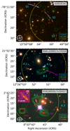 |
Fig. 1. Band 7 continuum contours for the three ACA pointings in this study on top of their respective HST color images. In all three panels, green solid (dashed) lines indicate positive (negative) contours of 870 μm imaging at the ±2, 3, 4, 5, 6σ levels. The yellow circle indicates the 20% sensitivity cut-off of the antenna primary beam. The white crossed ellipses at the lower left corners show the size of the synthesized beams. Upper panel: no significant detections are obtained within ACA data. Middle panel: two blobs of unambiguous emission are detected toward the center of the ACA beam, roughly cospatial with G1 and B1. Lower panel: four bright sources are detected at λ = 870 μm. Three of them are associated with A.1, A.2 and G1 respectively whereas the fourth source to the east is a previously unreported source (SMG). The inset shows a close-up view of a possible counterpart of the SMG in the WFC3-IR-F140W image (see Sect. 2.2.3). |
Both SGASJ0033-A and SGASJ1226-A are part of the Magellan Evolution of Galaxies Spectroscopic and Ultraviolet Reference Atlas (MegaSaura; Rigby et al. 2018), a catalog of moderate resolution rest-frame ultraviolet spectra of 15 gravitationally lensed galaxies at z ∼ 2 taken with the MagE instrument on the Magellan telescopes. The Sunburst Arc has comparable MagE data as part of the Extended MegaSaura Survey (Rigby et al., in prep.). The MegaSaura spectra provide secure spectroscopic redshifts as well as robust estimates on the age and metallicities of the young stellar populations (Chisholm et al. 2019). Unfortunately, a MagE spectrum for SGASJ1226-B is not available. In what follows, we adopt the stellar metallicity of SGASJ1226-B to be the same of SGASJ1226-A.
Promisingly, the James Webb Space Telescope (JWST) will target two of the sources presented here, namely SGASJ1226-A (ERS 1355, PIs: Rigby & Vieira) and the Sunburst Arc (GO 2555, PI: Rivera-Thorsen). The characterization we give here of the cold ISM in these galaxies will provide crucial insight to interpret the upcoming data.
2.2. Atacama Compact Array data
Our data includes observations with ACA obtained under ALMA program 2018.1.01142.S (PI: González-López). ACA – also known as the Morita Array – is a fixed configuration of twelve 7-meter antennas with a maximum baseline of 48.9 meters located at the Llano of Chajnantor (Iguchi et al. 2009). Our sources are lensed arcs that extend over several arcseconds on the sky, and ACA offers an optimal combination of an angular resolution that is high enough to deblend the sources while remaining sensible to large scale emission.
For all targets we set up observations to detect mid-J 12CO emission lines in ALMA Band 4 (ν ∼ 140 GHz) and continuum dust emission in ALMA Band 7 (ν ∼ 350 GHz). Mid-J transitions have been reported to be one of the brightest for most of SFGs (Carilli & Walter 2013; Daddi et al. 2015; Boogaard et al. 2020) while also providing information about the molecular gas budget. Band 7 observations, on the other hand, are regularly used to trace dust-obscured star formation and also molecular gas mass (e.g., Schinnerer et al. 2016; Scoville et al. 2017; Miettinen et al. 2017; Darvish et al. 2018; Casey et al. 2019; Magnelli et al. 2020). In addition, Band 7 photometry for sources at z ∼ 2.5 puts important constraints on their overall far-infrared (FIR) luminosity.
All ACA data were calibrated and reduced using the Common Astronomy Software Application1 (CASA; McMullin et al. 2007) version 5.4.0-70 following the standard pipeline scripts. We assumed a flux calibration accuracy of 10% throughout. All subsequent imaging was done with CASA task tclean and using natural weights to maximize signal-to-noise ratio (S/N). The resulting cubes and images are sampled at pixel size equal to 1/5 of beam minor axis, and the astrometry is expected to be accurate to  .
.
2.2.1. The Sunburst Arc
We used a standard continuum setup for observing the Sunburst Arc with Band 7 receivers. This comprises a total of four spectral windows with 31.250 MHz wide channels. Two adjacent spectral windows cover from 335.504 to 339.426 GHz and the other two from 347.504 to 351.483 GHz.
From the observed visibilities, we performed dirty imaging in multifrequency synthesis mode. The process yielded a synthesized beam of  with position angle (PA) of
  . The resulting continuum intensity map achieved a root-mean-square (rms) sensitivity of 1σ ≃ 245 μJy over a total bandwidth of 7.5 GHz and 145 min on source. We found no peaks higher than 3σ within the primary beam (43′ in diameter), accounting for a nondetection of the arc in this experiment (see Fig. 1).
The spectral configuration for Band 4 included two main spectral windows. The first one was tuned to the frequency of the 12CO(4 → 3) transition at z = 2.37, covering from 134.472 to 137.469 GHz at a channel resolution of 3.904 MHz (equivalent to 8.5 km s−1 at the CO central frequency). The other one targeted the [C I]1→0 atomic line by covering from 145.553 to 147.526 GHz at the same resolution (8 km s−1). The setup also included two adjacent sidebands to constrain the underlying continuum emission.
We then synthesized data-cubes keeping the native channel resolution (3.9 MHz). We reached a sensitivity of 1σ ≃ 2.1 mJy beam−1 per channel and a median synthesized beam of  (PA = −17°) for the 12CO(4 → 3) spectral window and
  (PA = −17°) for the [C I]1→0 spectral window. We found that the cube contains no evident emission line signatures, that is, none of the targeted lines were detected in this experiment. However, we found a tentative (≲3σ) detection of a continuum source over the S1 arc segment (see Fig. 1) after averaging all the channels, including the sidebands. We then repeated the imaging process excluding channels within 250 km s−1 to each side of the expected central frequency for the 12CO(4 → 3) and [C I]1→0 lines. To clean out the dirty beam we manually placed a 10″ mask over the peak and cleaned down to the 1σ level. The final image has a beam of
  (PA =
(PA =  ) and residual rms of 80.4 mJy beam−1 achieved with 226 min of on-source integration time.
2.2.2. SGASJ1226
For the SGASJ1226 system we used the same spectral setup used for Band 7 continuum detection in the Sunburst Arc, with the same coverage in frequency and spectral resolution. The synthesis of the dirty image revealed two sources with S/N greater than five: A 5.5σ peak that is cospatial with SGASJ1226-B.1 (southward of the BCG, Fig. 1), and a 6.2σ peak which we associate with a known Mg II absorber galaxy at z = 0.77 (Mortensen et al. 2021; Tejos et al. 2021, therein labeled SGASJ1226-G1). We cleaned the images by placing clean masks on top of the two detected sources and iterating down to 2σ level. The cleaned image allowed us to resolve both sources unambiguously with a synthesized beam size of  (PA = −57″) and rms of 1σ ≃ 170 mJy beam−1 obtained with 202 min of on-source integration time (see Fig. 1).
Due to the higher redshift of the SGASJ1226 source (z = 2.92), we used Band 4 receivers to observe only the 12CO(5 → 4) transition, as no other strong lines are expected at this redshift. Thus the setup covers with 3.9 MHz resolution (∼8 km s−1) from 145.034 to 146.905 GHz and from 146.894 to 148.765 GHz, with an effective overlap of three channels. The corresponding sidebands cover from 132.906 to 134.890 GHz and 134.905 to 136.890 GHz at a channel width of 31.25 MHz. We constructed the dirty cube using tclean in cube mode and using natural weighting of the visibilities. We get a median beam of  (PA = −70″) and a sensitivity of 1σ ≃ 3.3 mJy beam−1 per channel using a total of 145.3 min of on-source integration time. However the result showed no significant emission anywhere in the cube, nor in the channel-averaged image.
2.2.3. SGASJ0033
For SGASJ003341 we used again the standard Band 7 continuum setup configuration. The dirty image showed three bright sources within the primary beam (see Fig. 1). The first two are spatially coincident with the optical arc and a strong Mg II absorber at z = 1.17 (hereafter labeled SGASJ0033-G1, Ledoux et al., in prep.), respectively. The third one is a previously unreported, very bright (≳5 mJy) source with no evident optical counterpart. For this reason we refer to it as SGASJ0033-SMG (sub-millimeter galaxy). A tentative counterpart on that position is seen only in the near infrared WFC3/F140W image of the Hubble Space Telescope (HST; as shown in the inset of the third panel of Fig. 1), and not in the bluer filters. The lack of an optical detection further supports the idea that the object is a high-redshift dusty SFG. Then we cleaned the image to the 2σ level taking advantage of the automatic masking feature of tclean. With a total of 203 min of on-source integration time, the resulting image reached a continuum rms of 0.17 mJy beam−1, with a beam size of  (PA =
(PA =  ).
).
Band 4 spectral configuration is similar to the one used for PSZ1G311. We targeted the 12CO(4 → 3) line (expected to lie at 136 GHz at z = 2.39) on the first spectral window and the [C I]1→0 line (145.180 GHz at z = 2.39) on the second. The channel bandwidth of these spectral windows was 3.906 MHz or 8.6 km s−1 at 136 GHz. After flagging the channels were we expect the CO and [C I] lines to be, we performed first order continuum subtraction in the uv-plane using the CASA task uvcontsub, since this source is also a bright continuum emitter. We then carried out the imaging process with tclean using natural weighting and manually defined clean region boxes. With 202 min of on-source integration time, we achieve a sensitivity of 1σ ≃ 2.1 mJy beam−1 per channel and a median synthesized beam size of  at a PA of
  . Preliminary analysis revealed a 10σ detection of the CO line and a 4σ detection of [C I], both cospatial with the optical arc. We also report the detection of a broad (∼400 km s−1) emission line at ν = 135.6 GHz, roughly cospatial with SGASJ0033-SMG (see lower panels of Fig. 2).
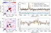 |
Fig. 2. Zeroth moment maps and spectra of the emission lines detected in Band 4 toward SGASJ0033. The upper panels show the integrated brightness map of the 12CO(4 → 3) line (left) and its spectral profile (right) observed over images 1 and 2 of the lensed galaxy SGASJ0033-A at z = 2.39. Black contours in both the upper left and lower left panels indicate the positive 870 μm continuum emission above 3σ already shown in Fig. 1. The black crossed ellipses indicate the size of the synthesized beam while the gray dashed ellipses show the apertures used for extracting the spectra shown in the corresponding right panel. The spectrum of 12CO(4 → 3) at A.1+A.2 (upper right panel) was resampled to a channel width of 12.5 km s−1; its best single Gaussian fit (see main text) is displayed in a red solid line. A tentative excess of emission at 150 km s−1 is highlighted by a red vertical arrow. Normalized residuals from the difference between the observed spectrum and the model are shown in blue in the subplot below. The lower panels show the moment map (left) and spectrum (right) of the serendipitous emission line which we associate to the SMG. The channel width was resampled to 30 km s−1 in order to maximize signal-to-noise while keeping five channels per FWHM. The spectral axis is in the same velocity frame as the spectrum of A.1+A.2 (νrest = 135.996 GHz). This choice highlights the proximity in velocity space of the two lines. |
2.3. Ancillary data
2.3.1. HST data
The three lensing clusters have been observed with the HST at multiple wide band filters. We retrieved the available data from the Mikulski Archive for Space Telescopes2 (MAST) to perform photometric extraction of each source in order to constrain their spectral energy distribution (SED). The PSZ1G311 field was observed in bands F606W and F160W with the Wide Field Camera 3 (WFC3; GO15377, PI: Bayliss), and the F814W filter with the Advanced Camera for Surveys (ACS; GO15101, PI: Dahle). For SGASJ1226, bands F110W and F160W of the near infrared channel of WFC3 were available (GO15378, PI: Bayliss), as well as bands F606W and F814W with the ACS (GO12368, PI: Morris). Finally, data for SGASJ0033 comprises bands F555W, F814W, F105W and F140W taken with the WFC3 (GO14170, PI: Wuyts). All imaging data were aligned with DRIZZLEPAC routine tweakreg, and drizzled to a common pixel size of  with astrodrizzle using Gaussian kernels with drop size of 0.8. We performed additional cosmic ray removal in Sunburst Arc’s F606W drizzled frame using ASTROSCRAPPY (McCully et al. 2018). As a last step, we check the absolute astrometric accuracy of our WCS solution by comparing the centroid positon of foreground stars in the drizzled images with the Gaia DR2 catalog (Gaia Collaboration 2018). We find no systematic offset nor rotation, and the observed shift is at most
  .
.
Since the lensed arcs are very extended in the sky and show complex morphologies, standard extraction routines are not well suited for obtaining reliable photometry of the sources. Instead, we employed ad-hoc polygonal apertures defined in the filter with the largest PSF for each target. We note that the background in SGASJ1226 and SGASJ0033 is dominated by the light from the brightest cluster galaxy (BCG) or other bright members of the foreground cluster. For this reason, we modeled the two elliptical isophotes of the BCG that encompass the arc extent, to isolate an area with similar contamination and background level as the source. Then we randomly placed two thousand 10 pixel wide apertures between these two isophotes and we take the resulting flux mean and variance as the background level and noise variance respectively for the science aperture, after properly scaling for the aperture area. For the Sunburst Arc, we used rectangular apertures enclosing each of the main arc segments. We estimated the background in nearby sky regions to each side of the arc.
2.3.2. Spitzer
Observing programs #70154 (PI: Gladders) and #13111 (PI: Dahle) of the Spitzer Space Telescope include observations of SGASJ1226 and the Sunburst Arc respectively, at 3.6 μm and 4.5 μm wavelengths using the Infrared Array Camera (IRAC). At z ∼ 3 these bands trace the older stellar populations of the source galaxies and hence are very important for constraining their total stellar mass. We retrieve the IRAC mosaics from the NASA/IPAC Infrared Science Archive reduced with the stock calibration pipeline.
Photometry for SGASJ1226-A.1 was obtained following the method outlined in Saintonge et al. (2013): using curve of growth arguments, we determine the optimal sized circular aperture and background annulus for computing the flux of SGASJ1226-A.1. The measured flux is 54 ± 11 μJy and 47 ± 9 μJy at 3.6 μm and 4.5 μm respectively. These values agree with the ones reported by Saintonge et al. (2013), 52.8 ± 6.0 μJy and 47.2 ± 4.2 μJy. The extraction of the southern arc, SGASJ1226-B, required a segment of an annulus instead of a circular aperture due to its larger extension. The annulus was centered on the core of the BCG and the complementary segment was used for background subtraction. The resulting image plane fluxes are 46 ± 13 μJy at 3.6 μm and 44 ± 8 μJy at 4.5 μm.
Unfortunately, the Sunburst Arc field suffers from severe crowding, and the arc appears blended with foreground galaxies and stars at the IRAC resolution. Thus, aperture photometry was not an option in this case. To avoid the introduction of additional uncertainties and assumptions, we did not attempt a prior-based PSF-fitting approach, but completely exclude these two bands from the analysis.
The effect on the determination of stellar mass when the IRAC bands are not included in the SED fitting was explored in Mitchell et al. (2013) by analyzing mock galaxy SEDs with known physical parameters. In that study, the exclusion of IRAC bands resulted in a bias in Mstars of −0.04 and −0.03 dex at z = 2 and z = 3, respectively, after removing the contribution from dust and metallicity effects. The scatter in the recovered Mstars is, however, on the order of 0.1 dex. Although these values were obtained in the idealized situation where the SED fitting code matches the IMF and stellar population model used for generating the SED, we can interpret them as an indication that our Mstars estimate for SGASJ0033-A and the Sunburst Arc has larger uncertainties but not a significant bias. As a complementary test, we ran MAGPHYS on SGASJ1226-A and SGASJ1226-B again but turning off the fitting for the IRAC bands. The median value of the marginal posterior probability distribution for Mstars was +0.02 and −0.11 dex for SGASJ1226-A and SGASJ1226-B, respectively, relative to the fiducial values listed in Table 4. In both cases, the offset is much smaller than the uncertainty returned by the code. This again indicates that the lack of IRAC bands only affects the uncertainty but not the nominal value.
2.3.3. Lens models and source plane reconstruction
Lens models for the three clusters were developed with the parametric LENSTOOL (Jullo & Kneib 2009) software based on identification of multiple images of the same lensed features in the HST imaging data, following the same methodology detailed in Sharon et al. (2020). The models consist of a collection of parametric dark matter halo profiles centered on the cluster galaxies and assuming all members lie on the same plane (thin lens approximation). Once a set of parameters that minimize the spatial offset between predicted and observed image pairs is obtained, the best fit model provides the deflection matrices and magnification maps that are used to reconstruct the source plane properties of the lensed galaxies. The models for the three lensing clusters in this work were already published in the literature and all of them were fit with at least 10 lensing constraints, including features in the giant arcs as well as other multiply-imaged sources at different redshifts. We refer the reader to the following references for details on each model: the lens model for the PSZ1G311 cluster is published in Rivera-Thorsen et al. (2019); for the SGASJ1226 cluster, in Dai et al. (2020) and Tejos et al. (2021); and for SGASJ0033, in Fischer et al. (2019).
Throughout this paper, we report average magnifications computed as the area ratio between the image plane and the source plane within a given aperture defined in the image plane. Whenever the aperture includes multiple images, the magnification factor μ accounts for this to match the source plane area of the image with the largest footprint. For example, the arc SGASJ1226-A.1 is divided into two images by the lensing critical line. Each half maps to the same (partial) region of the source galaxy. SGASJ1226-A.2, on the other hand, is a less magnified version of the whole source galaxy, as it has a larger footprint in the source plane. Then, we set the magnification factor so that the joint image plane area of both halves of SGASJ1226-A.1 divided by μ yielded the source plane area of SGASJ1226-A.2. We adopted an uncertainty on magnification of 20% for all images to account for the statistical error in cluster lens modeling. We note, however, that the uncertainties are possibly dominated by systematics (e.g., Raney et al. 2020).
An advantage of observing this kind of systems with millimeter and submillimeter interferometers is that the model to be used is developed from independent data. Models created with deep optical images can be used to interpret the observed emission, avoiding the use of the same data to characterize the models. This approach has proven to be the only reliable method for dealing with cluster-scale strong lensing (e.g., Saintonge et al. 2013; González-López et al. 2017a; Laporte et al. 2017; Sharon et al. 2019; Dessauges-Zavadsky et al. 2019). However, it is important to acknowledge that several studies of galaxy-scale systems – which have a single or very few lensing halos – have successfully used the interferometric data alone to fit lens models, provided such data reaches high angular resolution (e.g., Hezaveh et al. 2013; Bussmann et al. 2013; Messias et al. 2014; Rybak et al. 2015a,b; Spilker et al. 2016; Apostolovski et al. 2019; Rizzo et al. 2020)
3. Data analysis and results
3.1. Emission lines in the SGASJ0033 system
To search for lower S/N emission lines within the ACA cubes, we conducted two experiments: first, we selected and integrated along the velocity axis the channels where lines are expected according to redshift priors from literature (e.g., Koester et al. 2010; Tejos et al. 2021) using a fixed width of 200 km s−1. We retrieved the frequencies of the expected lines at each redshift prior using the web-based SPLATALOGUE3 tool. This experiment resulted in no detections above 3σ, other than the lines that were already identified (see Sect. 2.2). For the second experiment we proceed with a blind search of emission lines, via the automated LINESEEKER software González-López et al. (2017b); González-López et al. (2019). Again, we found no detections within the SGASJ1226 and the Sunburst Arc Band 4 cubes. The software correctly identified two of the three lines in SGASJ0033 already detected by visual inspection: the bright 12CO(4 → 3) line associated with the arc (SGASJ0033-A) and the dimmer but broader emission feature at 135.6 GHz toward the south east (SMG). LINESEEKER did not detect the [C I] line, however we consider it a reliable signal based on the strong priors on the frequency, position an width imposed by the 12CO(4 → 3) line. To confirm the detection, we extracted the [C I] spectrum from the same spatial region as the CO line and convolve it with the best fit Gaussian profile of CO, resulting in a peak correlation ∼25 km s−1 redward of CO’s central velocity (see Fig. 3).
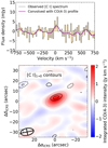 |
Fig. 3. ACA Detection of [C I]1 → 0 at z = 2.39 toward the lensed galaxy SGASJ0033-A. Upper panel: continuum subtracted spectrum at 145 GHz extracted from the A.1+A.2 aperture (dashed gray line in lower panel) with 2 channel binning (gray line). The overlaid purple curve is the result of the convolution between the observed spectrum and a Gaussian kernel with FWHM equal to the best fit value of the 12CO(4 → 3) line. The velocity axis is centered at the redshift of 12CO(4 → 3). Lower panel: integrated [C I] emission contours (black solid/dahsed curves) at the ±2, 3σ levels on top of the 12CO(4 → 3) moment map. The crossed ellipse at the lower left corner indicates the size and orientation of the [C I] beam. |
To extract line width and central velocity, we fit one dimensional Gaussian profiles to the CO spectra of SGASJ0033-A and SGASJ0033-SMG using non linear least squares minimization. Motivated by the marginal asymmetry of the line (see upper right panel of Fig. 2) and the recent discovery of broad velocity components of nebular, rest-frame optical lines in this object (Fischer et al. 2019), we tested for the presence of a similar feature in the observed CO profile. We fit single, double and triple Gaussian models, but only the single Gaussian achieved optimal corrected Akaike Information criterion (AICc; Cavanaugh 1997) and Bayesian Information criterion (BIC; Wit & Heuvel 2012) scores. These scores calculate a goodness-of-fit estimate (e.g., χ2) but penalize overfitting by taking into account the number of degrees of freedom of the model. According to these criteria, double and triple Gaussian models are not as significant as the single Gaussian model. Thus, the results indicate no evidence of broad nor high velocity components within current data.
The total flux for each line was computed from the velocity integrated intensity maps (zeroth moment). Centered at the best fit central frequency, we used symmetric integration ranges spanning from −0.85 to +0.85 times the best-fit Gaussian FWHM. In this way we recover ∼99.5% of the flux while keeping S/N ≳ 3 per channel. The resulting moment maps were then fit with a 2D Gaussian profile using CASA task imfit, using the coordinates of the peak pixel as a prior on their position. The inferred fluxes with their respective uncertainties are listed in Table 3. The results of the fits are consistent with the sources being unresolved by the ACA Band 4 beam. For the CO nondetections (SGASJ1226-A, SGASJ1226-B and Sunburst Arc) we report 3σ point source upper limits assuming a fixed integration range width of 200 km s−1 around the best spectroscopic redshift available.
3.2. Continuum photometry
The flux of the 870 μm continuum detection was determined in a similar way to the CO line flux (see Sect. 3.1): we fit single 2D Gaussians to each source using imfit on the cleaned continuum maps. In this case, the SGASJ0033 arc A.1 is resolved from the counter-image A.2 so we employed one Gaussian for each image. The (image plane) size of the best fit model for A.1 indicate that the arc is partially resolved along the major axis. Again, for the targets that were not detected, we quote the 3σ upper-limit for point sources based on the observed rms and corrected by primary beam attenuation. We also measured the continuum flux on Band 4 (λobs = 2.1 mm) data in a similar fashion. First we built dirty images after masking out the channels with detected and undetected line emission. Once again, SGASJ0033 is the only source with a reliable signal. The results are presented in Table 2.
Summary of selected target and ACA observations.
ACA continuum photometry in bands 7 and 4.
3.3. SED fitting
We combined image plane optical HST photometry (four bands), ACA submillimeter continuum photometry (two bands) and IRAC near infrared photometry (two bands) when available to fit templates of spectral energy distributions (SEDs) and derive estimates of stellar mass and star formation rate. For this purpose, we used the high-z version of the Multi-wavelength Analysis of Galaxy Physical Properties package (MAGPHYS; da Cunha et al. 2015). MAGPHYS uses precomputed grids of stellar emission (Bruzual & Charlot 2003) and dust emission models (da Cunha et al. 2008) to evaluate the likelihood that the observed multi-band photometry comes from each combination of stars plus dust models. The results are given as samples of the posterior probability distribution of the parameters of the models. The code operates under the principle of energy balance, which states that all the energy of the UV radiation field absorbed by the dust in the interstellar medium is re-emitted in the far infrared as a thermal continuum. When both the UV and FIR fluxes are observed, and a given attenuation law is assumed (in the case of MAGPHYS, Charlot & Fall 2000), this principle provides a useful constraint that can break the degeneracies associated with galaxy reddening. Still, with no data in the mid infrared and a low total number of bands observed, SED fitting suffers from large uncertainties (e.g., from the unconstrained contribution of AGN). In order to address possible systematics we also ran CIGALE (Boquien et al. 2019), another SED fitting code, and then compare with our MAGPHYS results. CIGALE allows more flexibility in the modeling choices, like the shape of the star formation history (SFH), the attenuation law or the inclusion of other components like radio synchrotron emission. For this experiment, we used the same stellar templates and attenuation law as MAGPHYS, but assumed a delayed exponential SFH and a nebular emission component (based on templates by Inoue 2011). We also used the simpler dust emission model proposed by Dale et al. (2014), which is a grid of templates that depend on two parameters: αSF, which governs the strength of the dust heating intensity, and fAGN, the AGN fraction. Here we have chosen to fix fAGN = 0 and vary αSF between 0 and 4. We found that both CIGALE and MAGPHYS offer reasonable fits to the observed bands, but the former produces on average ∼0.15 dex and ∼0.3 dex higher estimates of SFR and Mstars respectively than MAGPHYS. These differences are consistent with the results of a comparison between MAGPHYS masses and EAGLE/SKIRT simulated galaxies (Dudzevičiūtė et al. 2020). However, the Bayesian posterior probability distributions of these parameters produced by either codes do overlap within their 68% confidence intervals (see Fig. 4 for an example), so we do not consider the differences to be statistically significant. In what follows, we report MAGPHYS derived values corrected by magnification (see Table 4).
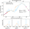 |
Fig. 4. Example SED fit for the lensed galaxy in SGASJ0033. Purple circles show the magnified image plane photometry from HST and ACA. The bottom panels show the posterior probability distributions for three model properties, comparing the MAGPHYS and CIGALE solutions. The lack of mid-infrared photometry leads to significant discrepancies between the two models between rest-frame 2 μm and 250 μm. |
Emission line properties toward SGASJ0033.
Physical properties derived from SED fitting and dust masses from far-infrared photometry.
3.4. Dust mass
The MAGPHYS fits to the far infrared SED deliver posterior probability distributions of the total dust mass, but since that part of the SED is sparsely sampled (single band detection or upper limits) the uncertainties are large. An alternative way to estimate the dust mass directly from the single band sub-millimetric flux is by using the framework proposed by Dunne et al. (2000). This method is based on the assumption that optically thin dust traces the cold ISM, and therefore the observed continuum flux is proportional to the dust mass (e.g., Eales et al. 2012; Scoville et al. 2014, 2016). Following Scoville et al. (2016), we set the global mass-weighted dust temperature to Td = 25 K and the dust emissivity index to β = 1.8. Then, the dust mass is computed as,
 (1)
(1)
where νobs is the observed frequency, Sνobs the measured flux and DL the luminosity distance. The quantity κ(νref) is the dust mass absorption coefficient at rest frame νref; here we adopted κ(450 μm) = 1.3 cm2 g−1 (Li & Draine 2001). Bν is the Planck function and ΓRJ(ν, z, Td) is a factor that accounts for the deviation of the Planck function from the Rayleigh-Jeans (RJ) law. The intrinsic dust masses (or upper limits) obtained with this method are presented alongside the SED results in Table 4.
The validity of this method relies on the restriction λrest > 250 μm, which ensures that one is probing the Rayleigh-Jeans tail and dust is optically thin (Scoville et al. 2016). Here, the condition is met for SGASJ0033 and the Sunburst Arc, but not for the SGASJ1226 galaxies since 870 μm at z = 2.92 becomes 222 μm. However, low metallicity galaxies –like SGASJ1226-A and B– typically have higher dust temperatures than their solar metallicity equivalents at fixed redshift (Rémy-Ruyer et al. 2013; Saintonge et al. 2013). In such cases, the SED peak and Rayleigh-Jeans tail are shifted toward shorter wavelengths, hence relaxing the λrest restriction. Also, the calibration of Scoville et al. (2016) did include 870 μm flux measurements of SMGs at z ≳ 2.5, since they were found to follow the same  trend as local spirals and ULIRGs. For these two reasons, we believe that λobs = 870 μm remains a good tracer of dust mass for the two lensed galaxies in the SGASJ1226 system, and the method outlined above still applies. In any case, we repeated the measurement with the Band 4 continuum (λobs = 2.1 mm), obtaining a very similar value for SGASJ0033 as with 870 μm (
 vs.
vs.  ), though with higher uncertainty. Despite tracing a rest-wavelength that is well within the RJ regime and closer to the reference wavelength of 850 μm, the 2.1 mm continuum is expected to be much fainter than 870 μm at these redshifts, hence the upper limits obtained with Band 4 measurements are less restrictive (see Fig. 5).
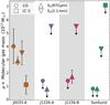 |
Fig. 5. Measurements and upper estimates on image plane molecular gas mass according to different tracers. The gray background strips serve as a visual aid to separate the different sources. The molecular gas mass measurements of SGASJ0033 based on CO and dust continuum are consistent with each other, while the [C I] based estimate favors a lower value. |
3.5. Molecular gas mass
A major goal of this paper is to constrain the molecular gas content of the source galaxies producing the giant arcs. To estimate the global molecular gas mass, we employ at least one of the following methods:
-
(i)
Based on12CO(J → J − 1) luminosity: the observed CO line flux can be converted to the ground transition 12CO(1 → 0) luminosity, which is the traditional and best calibrated H2 tracer. To correct for the excitation level, here we adopt the median ratios
 from Kirkpatrick et al. (2019) calibrated in a sample of matched redshift and intrinsic infrared luminosity. Once
  is computed, we apply the Genzel et al. (2015) recipe for estimating the CO-to-H2 conversion factor (hereafter αCO) based on gas-phase metallicity. Without a homogeneous metallicity indicator for every target, we adopt the stellar metallicities reported by Chisholm et al. (2019) as a proxy. A discussion on the validity of this choice can be found in Appendix A.
 -
(ii)
Based on Mdust: giant molecular clouds in the ISM of star-forming galaxies contain cold dust that can be detected in long-wavelength thermal continuum emission (Eales et al. 2012; Magdis et al. 2012). With a measurement of the dust mass available (see Sect. 3.4), one can use the gas-to-dust mass ratio (δGDR = Mmol/Mdust) to infer the total molecular mass (Scoville et al. 2016). Here we adopt a scaling with gas-phase metallicity as δGDR ∝ Zγ, normalized at δGDR(Z⊙) = 100 (Draine et al. 2007) and a power-law index γ = −0.85 taken from Tacconi et al. (2018). This calibration should be valid for solar to slightly subsolar metallicities (Leroy et al. 2011; Rémy-Ruyer et al. 2014), but will be revisited in Sect. 4.3. As presented in Sect. 3.4, we derive dust mass from both Band 7 (870 μm) and Band 4 (2.1 mm) continuum.
-
(iii)
Based on [C I]1→0 luminosity: the fine structure lines of atomic carbon have been proposed as reliable tracers of cold gas (e.g., Papadopoulos et al. 2004; Danielson et al. 2011; Popping et al. 2017). In order to convert [C I]1→0 luminosity to H2 mass one first has to compute the total atomic carbon mass. Since both 3P2→3P1 and 3P1→3P0 lines are optically thin and have low critical densities, the mass only depends on the luminosity and excitation temperature Tex (Weiß et al. 2003, 2005). The excitation temperature can be estimated from the luminosity ratio of both transitions, but since our data only covers the 3P1→3P0 transition, we set Tex = 30 K as typically assumed in the literature (e.g., Bothwell et al. 2017; Popping et al. 2017; Valentino et al. 2018; Brisbin et al. 2019; Boogaard et al. 2020, 2021. At Tex = 30 K, a 20% variation in temperature produces a ≲1% variation in M[CI] (Weiß et al. 2005; Boogaard et al. 2020). Once the atomic carbon mass has been computed (i.e., with Eq. (1) of Weiß et al. 2005), we use the metallicity dependent prescription of Heintz & Watson (2020) for the carbon abundance to convert to molecular gas mass. Unlike method (ii) whose δGDR(Z) scaling is calibrated on CO-derived gas masses, the Heintz & Watson (2020) relation was obtained directly from the [C I]/H2 column density ratio observed in a sample of quasar and gamma ray burst absorbers at high-z, and hence is independent of the αCO factor. For this reason, the [C I]-based Mmol provides useful consistency checks on the previous two methods.
Since SGASJ0033-A has detections of CO, [C I] and dust continuum, we can use it as a benchmark for the three methods listed above. Following method (i) we adopted r41 = 0.37 ± 0.12 (from Kirkpatrick et al. 2019) and αCO = (4.5±0.1) M⊙ (K km s−1 pc2)−1 based in our fiducial metallicity Z/Z⊙ = 0.84 ± 0.02 (Appendix A). We then converted the observed image plane CO flux into  , where A.1 + A.2 indicates that the value considers the blended flux of the two lensed images. With δGDR(Z) = 117 and X[CI](Z) = 1.3 ± 0.8 × 10⁻⁵ (for reference, the typical value assumed for high-z studies is 3 × 10⁻⁵, Valentino et al. 2018) results from methods (ii) and (iii) are
  and
and ![Mathematical equation: $ \mu M_{\mathrm{mol, [CI]}}^{A.1+A.2} = (1.1\pm0.7)\times10^{11}\,{M_\odot} $](/articles/aa/full_html/2021/11/aa41835-21/aa41835-21-eq55.gif) respectively. While the values obtained with methods (i) and (ii) are in reasonable agreement for both tracers of Mdust, the (iii) method yields an estimate that is ∼2σ lower. This can be a result of the low significance of the [C I] detection or a systematic effect driven by the uncertain carbon abundance factor. In what follows, we adopt the CO estimate as the fiducial value of Mmol for SGASJ0033-A.
respectively. While the values obtained with methods (i) and (ii) are in reasonable agreement for both tracers of Mdust, the (iii) method yields an estimate that is ∼2σ lower. This can be a result of the low significance of the [C I] detection or a systematic effect driven by the uncertain carbon abundance factor. In what follows, we adopt the CO estimate as the fiducial value of Mmol for SGASJ0033-A.
4. Discussion
4.1. Lensed galaxies in context
In order to locate our derived ISM properties of lensed galaxies within the context of high-z scaling relations, we compare our results with a pair of reference samples. The main reference sample is the latest release of the IRAM Plateau de Bure High-z Blue Sequence Survey (PHIBSS 1/2; Tacconi et al. 2013, 2018) containing 1444 molecular gas measurements at 0 ≤ z ≤ 4 and covering a stellar mass range from log(Mstars/M⊙) = 9 to 11.9. The sample includes both individual galaxies and stacked measurements from surveys with high detection rates. The sample was selected to represent the overall SFG population in a wide range of basic galaxy parameters. The bulk of the sample are galaxies that belong to the star-forming main sequence, with a modest contribution from star-bursting outliers (Tacconi et al. 2018). From this parent sample we selected two subsets: firstly, a high-z sample defined as all the sources in the PHIBSS 1/2 catalog with spectroscopic redshift greater than 2, excluding lensed galaxies. This subset contains 138 objects with stellar masses between 109.8 M⊙ and 1011.8 M⊙ and a median redshift of 2.3. The molecular gas masses were derived from CO luminosity for 59 sources and from dust continuum for the other 79 sources. Secondly, the entire xCOLD GASS sample (Saintonge et al. 2011) as appears in PHIBSS 1/2. It contains 306 galaxies at z ∼ 0 with CO measurements and stellar masses ranging from 109 to 1011.3 M⊙.
We also compiled a sample of molecular gas measurements in UV-bright strongly-lensed galaxies from S13 and DZ15. These two studies provide global properties and molecular gas masses for several giant arcs, most of them selected from optical surveys. In both studies, a complete sampling of the infrared SED with Spitzer and Herschel is combined with dedicated PdBI or IRAM 30m CO line observations to constrain the parameters of the cold ISM of these galaxies. After we remove duplicate objects between the two samples and exclude the SGASJ1226-A arc from the S13 table, this sample comprises 17 sources at mean redshift of z ≈ 2.1 and a delensed stellar mass range of 109.3 to 1011.5 M⊙.
Each sample uses their own set of calibrations and tracers for the molecular gas. On one hand, the PHIBSS catalog uses the G15 metallicity-dependent recipe for estimating αCO, while S13 used the Genzel et al. 2012 (G12) recipe. On the other hand, DZ15 assumed a constant Galactic value of αCO = 4.6 M⊙ (K km s−1 pc2)−1. Here, we attempted to standardize the reference samples to a common scheme for unbiased comparison with our sample. We updated the MH2 values in Table 6 of S13 to the G15 calibration based on the metallicities provided in their Table 5. With this calibration, the molecular gas mass estimations become 0.2 dex lower on average. For the DZ15 sample we retrieved metallicities from S13 for the duplicate sources cB58 and the Cosmic Eye. For the rest of their sample, we computed metallicities from the MZR as appears in G12 and then converted to the Denicoló et al. (2002) scale for consistency with S13. We finally applied the G15 recipe to get αCO and updated the reported values of Mmol accordingly. This resulted in ∼0.1 dex higher gas mass estimations relative to their published values.
We also checked that the STARBURST99 stellar metallicities from Chisholm et al. (2019) in our sample are consistent with the expectations from the mass metallicity relation (MZR; see Sect. 1): we fed the SED-derived stellar masses into the MZR recipe used by G12 and converted them to the Denicoló et al. (2002) scale. The resulting oxygen abundances are all within 0.2 dex of the Chisholm et al. (2019) value. Thus, even if the intrinsic scatter of the MZR is lower than 0.2 dex at these resdhifts, the deviations we observe are fully consistent with our Mstars uncertainty.
Figure 6 shows the ranges of stellar mass and star formation rate that become accessible with the help of strong gravitational lensing. Compared to the unlensed high-z PHIBSS1/2 sample, the lensed galaxies occupy a much wider range in both SFR and Mstars, while still being located near (within 1σ errors) the empirical MS proposed in T18. In particular, the four sources in our sample have stellar masses well within the range of the z ∼ 0 SFGs represented by the xCOLD GASS sample, a regime not yet explored by unlensed surveys at this redshift.
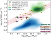 |
Fig. 6. Star formation rate versus stellar mass diagram for the lensed sources in this work, compared to literature samples. The PHIBSS1/2 subsamples are displayed as filled contours of Gaussian kernel density estimates, starting at the 20% peak density level. The solid line indicates the empirical location of the star-forming main sequence at z = 2.5 derived from PHIBSS1/2 data by Tacconi et al. (2018). The dashed lines and pale red filling indicate the typical ±0.3 dex scatter in this relation. Orange-filled triangles represent lensed galaxies from Saintonge et al. (2013) and Dessauges-Zavadsky et al. (2015). |
The ratio between the total molecular gas mass and the total stellar mass (hereafter gas fraction, Mmol/Mstars) is a crucial parameter to characterize the galaxy-integrated ISM properties, since it relates the amount of gas available to produce stars in relatively short timescales with the accumulated stellar mass buildup. There is a growing consensus that high-redshift galaxies have larger gas fractions than local galaxies for a given stellar mass (e.g., Scoville et al. 2017; Tacconi et al. 2018; Liu et al. 2019), a fact that might be explained by increased rates of gas accretion from the cosmic web at earlier times (e.g., Dekel et al. 2009; Walter et al. 2020). However, the current surveys of molecular gas at high redshift are not sensitive to lower mass (Mstars ≲ 1010 M⊙) systems (see Hodge & da Cunha 2020, for a review), so it remains unclear whether galaxies in this regime follow the same trends (e.g., Coogan et al. 2019; Boogaard et al. 2021).
In Fig. 7, we compare the gas fractions of our sample with the literature samples mentioned above. We observe that the z ∼ 2 lensed galaxies do, in fact, have larger gas fractions than the local xCOLD GASS sample, but these values are lower than expected for their redshift and mass range based on the extrapolation of the T18 relation. Our detections and upper limits reach values that are below the sensitivities of individual ALMA observations of low mass galaxies at z ≈ 2 (pink arrows; Coogan et al. 2019) and deep stacked measurements from the ASPECS survey (pale blue errorbars; Inami et al. 2020, using the values of the “on-MS” row of their Table 5).
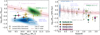 |
Fig. 7. Molecular gas fraction and depletion timescale (Mmol/SFR) in the context of high and low redshift galaxies. We only show our values based on the 870 μm band continuum as a tracer of Mmol, since it has the highest sensitivity and shows remarkable agreement with the CO-based values (see Fig. 5). The only exception is SGASJ0033-A for which we plot the CO-based value. Left: the filled green (blue) contours show the locus of the Gaussian kernel density estimator for the PHIBSS 1/2 z > 2 (xCOLD GASS) sample. Squares indicate the location of the lensed galaxies presented in this paper, identified by color in the right panel. We also include the joint sample from DZ15 and S13 as orange filled triangles. The brown solid and gray dotted lines show the Tacconi et al. (2018) scaling relation at z = 2.5 using the first and second order fits respectively. Pink downward arows at the top left are the upper limits from the CO nondetections presented in Coogan et al. (2019), while the pale blue errorbars are the result of deep CO stacking in the Hubble Ultra Deep Field with 1.0 < zspec < 1.7 in bins of one dex in Mstars (Inami et al. 2020, the bin with 8 < log10(Mstars/M⊙) < 9 is not shown). Right: gas depletion time versus redshift. The solid brown line is the T18 scaling relation for galaxies with Mstars = 109.7 M⊙, the median mass of our sample. PHIBSS 1/2 data is displayed as shaded circles instead of contours, but the darkness of each circle is a proxy of the number density. Again, the lensed sources studied here fall below the expected relation. The stacked upper limit from Inami et al. (2020) is also shown, and corresponds to the Mstars bin between 109 M⊙ and 1010 M⊙. |
In the left panel we see that gas fraction is anticorrelated with stellar mass for the high-z PHIBSS 1/2 galaxies, that is, more massive galaxies have relatively smaller gas reservoirs. In the stellar mass interval between 1010.3 M⊙ and 1011.5 M⊙, both the high-z and the local sample follow similar trends, but at lower masses, the local sample reveals a flattening of the relation. According to T18, this nonlinear behavior can be interpreted as a manifestation of the “mass-quenching” feature of the main sequence (suppression of SFR at high Mstars, e.g., Whitaker et al. 2014; Schreiber et al. 2015), though it has also been suggested that this is just a selection effect due to mass incompleteness (Liu et al. 2019). Here we show that the lensed galaxies distribute at log(Mmol/Mstars)≲ − 0.5, with no clear indication of Mstars dependence. Although the scatter is large and the number of sources small, the lensed galaxies have, on average, gas fractions one order of magnitude below the value one would obtain by extrapolating the linear T18 relation beyond the PHIBSS 1/2 mass range at z > 2. In detail, the offsets from the linear T18 (red line in Fig. 7) relation are 0.7, 0.8, > 1.2 and > 1.1 dex for SGASJ0033-A, SGASJ1226-B, SGASJ1226-A and the Sunburst Arc, respectively. An alternative second-order relation is also given in T18 (dotted gray line in Fig. 7), which accounts for the low mass flattening, but even with this correction the lensed galaxies show a lower gas fraction than predicted.
The right panel of Fig. 7, shows a comparison of the gas depletion timescale (Mmol/SFR) as a function of redshift. This plot also includes the intermediate-redshift sources we had excluded from the PHIBSS 1/2 subsample. While the scatter of points with respect to the T18 scaling relation is large (0.4 dex), the lensed galaxies from this work present gas depletion timescales that are shorter than expected based on the T18 relation by 0.6, 0.6, > 0.8 and > 0.8 dex for SGASJ0033-A, SGASJ1226-B, SGASJ1226-A and the Sunburst Arc, respectively. SGASJ0033-A is in agreement with other (albeit more massive) sources at the same redshift, but the tension is higher for the nondetected Sunburst Arc and SGASJ1226-A, whose gas will deplete in less than 100 Myr at the current SFR. Taken at face value, these results suggest that the lensed galaxies track a gas-deficient population that contrasts with the more massive galaxy population at high-redshift. In the following, we discuss on possible biases affecting the measurements.
4.2. The molecular gas deficit cannot be explained by systematics in Mstars or SFR
Before we can ascribe the observed deficit in the gas fraction and depletion time to the properties of the sampled galaxy population, we explore potential systematic effects on the measured quantities that can explain the discrepancy. For this, we temporarily adopt the hypothesis that our sample should strictly follow the T18 scaling relations. Under this hypothesis, the low gas fraction and depletion time can be driven, for example, by a systematic underestimation of the molecular gas mass, or conversely, by an overestimation of the stellar mass and SFR. In this section we focus on the latter effect, while a discussion on a possible underestimation of molecular gas mass is postponed to Sect. 4.3.
A shift on the measured stellar mass (keeping everything else constant) would need to be on the order of 0.7–1.2 dex to reconcile the observed gas fraction with T18. Some degree of offset in this direction could be achieved, for example, if MAGPHYS systematically overpredicts the stellar mass when the rest-frame near and mid infrared photometry are poorly constrained (da Cunha et al. 2015). However, if the measured metallicity is correct (see Appendix A), then a lower estimate of the stellar mass (e.g., from a different SED fitting code) will create tension with the MZR (as parameterized by Genzel et al. 2015). In other words, the T18 gas fraction relation favors a lower stellar mass whereas the MZR favors a higher stellar mass.
Another possibility to reconcile the measured gas fraction with T18 is that the magnification factor is systematically over-estimated: lower values of μ will displace points horizontally in the left panel of Fig. 7, since ratios of flux-dependent quantities cancel out the factor μ (under the assumption that the differential lensing effect is not too severe). But in the gas fraction versus stellar mass diagram the horizontal offsets from the T18 relation are at least ∼1 dex larger than the vertical offsets (listed in Sect. 4.1), so magnification alone cannot explain them. Even if we used the image plane uncorrected values (i.e., μ = 1), the square symbols in Fig. 7 would remain below the T18 relations.
However, in the high magnification regime, differential lensing can become significant. There are at least three geometrical conditions that can produce a higher magnification for the stellar component relative to the gas component, thus lowering the derived gas fraction: (1) if the UV emission from stars is spatially offset from the molecular gas reservoirs and closer to the lensing caustic lines; (2) if the stars’ brightness distribution is more compact than the gas distribution; or (3), with a combination of the previous two effects. The first condition is certainly possible, since spatial offsets between gas and stars are commonly observed in resolved studies of unlensed, high-redshift galaxies (Hodge & da Cunha 2020, and references therein). For example, Chen et al. (2015) found an average intrinsic scatter in the positional offsets between ALMA 870 μm detections and their HST counterparts of  , in a sample of 48 SMGs at z = 1 − 3. Similar offsets are found for other gas tracers such as CO lines (e.g., Calistro Rivera et al. 2018). But for any given system, the actual configuration of gas and stars is random and independent of the foreground lens. Even if we are selecting sources with a highly magnified stellar component, there is nothing in our selection function that favors a less magnified gas component. This means that, statistically, the magnification bias due to spatial offsets in the source plane plays in both directions and eventually cancels out. Then, based on spatial offsets alone, it is unlikely that both our lensed sources and the ones from S13 and DZ15 have a systematically more magnified stellar component. Most importantly, large offsets between unobscured UV emission and dust or gas tracer are preferentially seen in galaxies with high dust obscuration such as in GN20 (Hodge et al. 2015), but less commonly in low metallicity galaxies. Regarding the sizes of each component, observational evidence suggest that the background population will have a more compact dust component than the stellar component. This is true for both massive galaxies and intermediate mass galaxies (e.g., Fujimoto et al. 2017; Kaasinen et al. 2020). So if this was the case for the galaxies in our sample, it will drive larger magnifications for the gas component pushing the gas fraction to higher values, not lower. In conclusion, it is still possible to have a geometrical configuration of the source system in which lensing preferentially boosts the stellar component over the gas component, for example, with an extended gas distribution relative to stars coupled with a large spatial offset, but such configurations are extremely rare, making it unlikely to produce a systematic effect. Unfortunately, we cannot currently provide a quantitative estimation of the bias in the magnification. That will require matching HST resolution with ALMA observations of the gas/dust in the arcs.
Now, we consider the case where SFR is overestimated but Mstars is not. Then, at fixed Mmol, the depletion timescale appears lower than it actually is. Also, for a fixed stellar mass and redshift, T18 predicts higher gas fractions at higher SFR. Again, this effect can be due to MAGPHYS using priors that prefer templates with higher specific SFR (SFR/Mstars). But the best fit MAGPHYS models are already on or slightly below the T18 MS, so if the stellar masses are correct, then a lower value for the SFR will displace them even further from the MS, toward the locus of quenched galaxies. This is again an implausible scenario, for these galaxies have strong indications of star formation activity (e.g., young ages, blue colors, nebular emission lines, etc.).
Moreover, independent measures of stellar mass and SFR for some of the lensed galaxies in this work have been reported in the literature. For example, S13 found SGASJ1226-A to have log(μMstars/M⊙) = 11.32 ± 0.15 and log(μSFR/(M⊙ yr−1)) = 3.15 ± 0.08, which convert to 9.38 ± 0.15 and 1.2 ± 0.08 respectively when matched to our fiducial magnification μ = 87. While the SFR reported here is three times lower, the stellar mass is in excellent agreement. More recently, Vanzella et al. (2021) reported log(Mstars/M⊙)≈9.0 and log(SFR/(M⊙ yr−1)) ≈ 1 for the Sunburst galaxy, also consistent with our estimates within the uncertainties. The considerations above plus the agreement with values obtained by other teams suggest that the SED-derived quantities alone cannot account for the tension with T18 relations, thus disfavoring the hypothesis that they hold true in this region of the parameter space.
4.3. Low metallicity as the driver of the apparent gas deficit
If the cold gas deficit is not caused by a systematic overestimation of Mstars and SFR, then the conclusion is that the molecular gas mass might be underestimated. Before exploring this idea, we first note that the gas deficit is observed not only in the four galaxies in our sample, but also in the compilation of lensed sources from S13 and DZ15. Our results provide additional evidence for a divergence from standard scaling relations in intermediate- to low-mass SFGs at z ≳ 2. But this result is not exclusive to strongly lensed galaxies. For example, Coogan et al. (2019) put stringent upper limits on the molecular gas mass of five z ∼ 2 Lyman Break Galaxies (LBGs), with values that also challenge the scaling relations. More recently, Boogaard et al. (2021) used data from the ASPECS Large Program (e.g., Aravena et al. 2019) to constrain the gas content of 24 MUSE-selected SFGs at z = 3 − 4 in the Hubble Ultra Deep Field (HUDF). At the standard Galactic value for αCO, Boogaard et al. (2021) also obtain gas fractions upper limits which are in tension with scaling relations from T18 and Liu et al. (2019).
In both lensed and unlensed studies, metallicity is often pointed out as the main driver of these discrepancies. In particular, it seems that the effect of low metallicity has a stronger impact in the tracer-to-gas conversion factor than expected. In other words, the lack of CO, dust or neutral carbon emission in high-z galaxies may reflect a redshift evolution of αCO, δGDR, and X[C I], respectively. For example, at a fixed metallicity, αCO in a high-z SFG should be 5 to 30 times larger than in a local SFG in order to explain the deficit. Such high values of αCO can be produced by CO-faint gas: a decreased metal abundance implies fewer C and O atoms but also a lower proportion of dust grains (high δGDR), thus providing less shielding from the far-ultraviolet radiation that causes CO dissociation. As H2 is less impacted by this effect (e.g., Gnedin & Draine 2014), the abundance of CO relative to H2 becomes much lower (Bolatto et al. 2013). In the Milky Way, a significant amount of H2 resides outside the CO-bright cores of molecular clouds, as inferred from independent tracers such as γ-rays (Grenier et al. 2005). But in low-metallicity star-forming local dwarf galaxies the CO-faint gas is much more pervasive, filling the regions where most of the carbon is occupying its first ionized state. In such cases, CO emission cannot trace the bulk of the molecular gas budget and the [C II] 158 μm line emerges as an alternative tracer (e.g., Wolfire et al. 2010; Glover & Clark 2012; Schruba et al. 2012; Amorín et al. 2016; Madden et al. 2020).
In principle, αCO(Z) should account for the CO-faint gas at low metallicity, but several prescriptions exist in the literature and there is no consensus on the slope of the relation. While most of the published recipes agree that αCO,MW ≈ 4.5 M⊙ (K km s−1 pc2)−1 at solar metallicity, the dispersion is very large at lower metallicities. The power-law index γ can vary from −0.65 (Narayanan et al. 2010) to −3.39 (Madden et al. 2020), but only the steeper laws (γ ≲ −2.0, normalized to αCO(Z⊙) = αCO, MW) are able to boost Mmol up to ∼1.2 dex at the metallicity range studied here. Using such recipes (e.g., Schruba et al. 2012; Madden et al. 2020) could put our galaxies closer to the scaling relations found for the gas fraction and depletion time, especially for the SGASJ1226 system which has the lowest metallicities.
A similar argument can be made regarding δGDR. In both observations of local galaxies and predictions from ISM models δGDR is found to increase inversely proportional to Z, with a power-law index close to unity (γGDR ≈ −0.85; Leroy et al. 2011; Magdis et al. 2012; Sandstrom et al. 2013). Other authors find that the scaling steepens at lower metallicity and thus a double power-law is best suited (Rémy-Ruyer et al. 2014). At higher redshift, studies of low mass galaxies have shown that either a shift in normalization (S13; DZ15) or a steeper relation is needed to account for the low dust luminosity observed (Coogan et al. 2019).
Finally, large uncertainties also affect the determination of the neutral carbon abundance X[C I] calibration. On one hand, theoretical prescriptions are strongly sensitive to modeling choices, such as the physics of cosmic rays and molecular cloud evolutionary states (Hodge & da Cunha 2020, and references therein). On the other hand, fully empirical calibrations are not yet available. ALMA is starting to fill the gap with observations of [C I] emission in the local (e.g., Crocker et al. 2019) and distant (e.g., Valentino et al. 2018) Universe, but those results are still dependent on CO or dust-based estimates of Mmol, which suffer from the aforementioned uncertainties. Here we have used a recipe that was calibrated independently from CO, but has some other caveats: Heintz & Watson (2020) used a small sample of quasar and gamma ray burst absorbers with abundance measurements of both C I* and H2. Absorption lines yield line-of-sight column densities, rather than surface densities, so the authors assume that the ratio between column densities of C I and H2 is equal to the surface density ratio. Furthermore, a single line of sight does not necessarily probes all the phases and conditions where neutral carbon and H2 coexist. Metallicities are also derived in absorption, hence are not directly comparable to the standard nebular emission line determination of oxygen abundances.
Given the large dispersion in tracer-to-gas calibrations in the subsolar metallicity regime and the small size of our sample, it remains difficult to falsify the hypothesis proposed above. In other words, the molecular gas scaling relations of massive galaxies at high redshift may not apply to lower mass galaxies. For example, one could envision a scenario in which recent starburst consumed or dispersed most of the gas available. But this claim cannot be confirmed without a more systematic calibration of gas tracers. Deciding whether the gas deficit in SFGs with Mstars ≲ 1010 M⊙ is real will require larger samples and deeper integration times using the full ALMA array, even with the aid of strong lensing.
5. Summary and conclusions
In this paper, we have reported ACA observations of the molecular gas on four star-forming systems at z ≳ 2.5 that are strongly-lensed by foreground clusters and were selected as bright giant arcs in the optical. We used different methods and tracers, in order to assess possible systematic effects. The resulting detections and upper limits, in combination with ancillary multiwavelength data, allowed us to characterize the global properties of the cold ISM such as gas fraction and gas depletion timescale in these galaxies compared to existing scaling relations.
Out of four galaxies of similar masses and SFR, only the most massive, SGASJ0033, was detected in CO(4–3), [C I]1→0 and dust continuum emission (see Fig. 2). The galaxy exhibits a very narrow (FWHM ≈ 85 km s−1) line profile coupled with a low significance asymmetric wing at high velocity. The highly magnified SGASJ1226-A was not detected in either CO(5–4) nor dust continuum. Instead, a companion lensed galaxy at the same redshift, SGASJ1226-B, was detected in Band 7 continuum (see Fig. 1) implying larger amounts of gas than in the A component. Also, no detections were made toward the extremely bright giant arc known as the Sunburst Arc. However, due to the high magnification of the source, the intrinsic upper limits can probe down to 109 M⊙ in molecular gas mass (assuming the typical tracer-to-gas calibrations, see Fig. 5). Remarkably, this result implies a gas depletion timescale shorter than ∼70 Myr.
The inferred gas fraction in the sample is higher than in z = 0 SFGs, in agreement with the trend of increasing gas fraction at high redshift. However, the gas fraction is roughly 0.5–1.0 dex lower than predicted by the Tacconi et al. (2018, hereafter T18) scaling relations based on stellar mass, redshift and offset from the MS (see Fig. 7). Similarly, gas depletion timescale is also below the expected value based in the T18 relation but with a milder offset. The lensed galaxies studied here lie only ∼0.6 to ∼0.8 dex below the locus of more massive unlensed galaxies at the same redshifts (see Fig. 7).
To investigate whether the apparent gas deficit is real, we explored systematic offsets that could be driving it. We find that the result is not strongly affected by systematic effects on SED fitting, as it would take unrealistic offsets in Mstars and SFR to drive the measured discrepancies with the scaling relations. We also explore the effect of differential lensing, but we conclude that it is unlikely to drive a large systematic offset in our sample of lensed galaxies plus the ones from literature. We propose that the apparent gas deficit is rather due to systematic uncertainties in the tracer-to-gas conversion factor dependence on metallicity. Our results favor a scenario in which the emission of CO, dust continuum, and [C I] are more strongly suppressed than what typical calibrations predict. Of course, this does not rule out the possibility of these galaxies actually have less gas than expected, due for example, to recent starburst episodes having consumed most of the available gas.
Finally, we stress that in using shallow ACA observations in combination with the lensing effect of massive clusters, it is possible to detect the molecular gas in a Mstars ∼ 1010 M⊙ galaxy and to put constraints on the molecular gas content of less massive galaxies. Expanding this technique to a statistical sample of giant arcs will tell if the apparent gas deficit is a common feature in lower mass galaxies at high-redshift. However, in order to get accurate estimates of the molecular gas mass, it is necessary to build improved calibrations of the known tracers with respect to metallicity.
Acknowledgments
We thank the anonymous referee for the constructive feedback and helpful comments. We also thank Ian Smail for the feedback about the manuscript. This paper makes use of the following ALMA 7m array data: ADS/JAO.ALMA#2018.1.01142.S. ALMA is a partnership of ESO (representing its member states), NSF (USA) and NINS (Japan), together with NRC (Canada), MOST and ASIAA (Taiwan), and KASI (Republic of Korea), in cooperation with the Republic of Chile. The Joint ALMA Observatory is operated by ESO, AUI/NRAO and NAOJ. This research is also based on observations made with the NASA/ESA Hubble Space Telescope obtained from the Space Telescope Science Institute, which is operated by the Association of Universities for Research in Astronomy, Inc., under NASA contract NAS 5-26555. These observations are associated with programs 15377, 15101, 15378, 12368 and 14170. In addition, this paper has made use of Spitzer Space Telescope data from the NASA/IPAC Infrared Science Archive, which is funded by the National Aeronautics and Space Administration and operated by the California Institute of Technology. SL was funded by project FONDECYT 1191232. LFB was partially supported by CONICYT Project BASAL AFB-170002. MA acknowledges support from FONDECYT grant 1211951, CONICYT + PCI + Instituto Max Planck de Astronomia MPG190030 and CONICYT+PCI+REDES 190194. This research made use of Astropy, (http://www.astropy.org) a community-developed core Python package for Astronomy (Astropy Collaboration 2013, 2018). All figures were prepared using Matplotlib (Hunter 2007) and Seaborn (Waskom et al. 2020). The scaling relations used in this paper were obtained from convenience routines included in the A3COSMOS gas evolution library (https://ascl.net/1910.003) (Liu et al. 2019).
References
- ALMA Partnership (Vlahakis, C., et al.) 2015, ApJ, 808, L4 [Google Scholar]
- Amorín, R., Muñoz-Tuñón, C., Aguerri, J. A. L., & Planesas, P. 2016, A&A, 588, A23 [NASA ADS] [CrossRef] [EDP Sciences] [Google Scholar]
- Apostolovski, Y., Aravena, M., Anguita, T., et al. 2019, A&A, 628, A23 [NASA ADS] [CrossRef] [EDP Sciences] [Google Scholar]
- Aravena, M., Decarli, R., Gónzalez-López, J., et al. 2019, ApJ, 882, 136 [Google Scholar]
- Astropy Collaboration (Price-Whelan, A. M., et al.) 2018, AJ, 156, 123 [Google Scholar]
- Astropy Collaboration (Robitaille, T. P., et al.) 2013, A&A, 558, A33 [NASA ADS] [CrossRef] [EDP Sciences] [Google Scholar]
- Baker, A. J., Tacconi, L. J., Genzel, R., Lehnert, M. D., & Lutz, D. 2004, ApJ, 604, 125 [NASA ADS] [CrossRef] [Google Scholar]
- Baldwin, J. A., Phillips, M. M., & Terlevich, R. 1981, PASP, 93, 5 [Google Scholar]
- Blanton, M. R., Bershady, M. A., Abolfathi, B., et al. 2017, AJ, 154, 28 [Google Scholar]
- Bolatto, A. D., Leroy, A. K., Rosolowsky, E., Walter, F., & Blitz, L. 2008, ApJ, 686, 948 [NASA ADS] [CrossRef] [Google Scholar]
- Bolatto, A. D., Wolfire, M., & Leroy, A. K. 2013, ARA&A, 51, 207 [CrossRef] [Google Scholar]
- Boldrin, M., Giocoli, C., Meneghetti, M., & Moscardini, L. 2012, MNRAS, 427, 3134 [NASA ADS] [CrossRef] [Google Scholar]
- Boogaard, L. A., van der Werf, P., Weiss, A., et al. 2020, ApJ, 902, 109 [NASA ADS] [CrossRef] [Google Scholar]
- Boogaard, L. A., Bouwens, R. J., Riechers, D., et al. 2021, ApJ, submitted, [arXiv:2105.12489] [Google Scholar]
- Boquien, M., Burgarella, D., Roehlly, Y., et al. 2019, A&A, 622, A103 [NASA ADS] [CrossRef] [EDP Sciences] [Google Scholar]
- Bothwell, M. S., Aguirre, J. E., Aravena, M., et al. 2017, MNRAS, 466, 2825 [Google Scholar]
- Brisbin, D., Aravena, M., Daddi, E., et al. 2019, A&A, 628, A104 [EDP Sciences] [Google Scholar]
- Bruzual, G., & Charlot, S. 2003, MNRAS, 344, 1000 [NASA ADS] [CrossRef] [Google Scholar]
- Bussmann, R. S., Pérez-Fournon, I., Amber, S., et al. 2013, ApJ, 779, 25 [NASA ADS] [CrossRef] [Google Scholar]
- Cañameras, R., Nesvadba, N., Kneissl, R., et al. 2017, A&A, 604, A117 [Google Scholar]
- Calistro Rivera, G., Hodge, J. A., Smail, I., et al. 2018, ApJ, 863, 56 [Google Scholar]
- Carilli, C. L., & Walter, F. 2013, ARA&A, 51, 105 [NASA ADS] [CrossRef] [Google Scholar]
- Casey, C. M., Zavala, J. A., Aravena, M., et al. 2019, ApJ, 887, 55 [Google Scholar]
- Cavanaugh, J. E. 1997, Stat. Probab. Lett., 33, 201 [CrossRef] [Google Scholar]
- Chabrier, G. 2003, PASP, 115, 763 [Google Scholar]
- Charlot, S., & Fall, S. M. 2000, ApJ, 539, 718 [Google Scholar]
- Chen, C.-C., Smail, I., Swinbank, A. M., et al. 2015, ApJ, 799, 194 [NASA ADS] [CrossRef] [Google Scholar]
- Chisholm, J., Rigby, J. R., Bayliss, M., et al. 2019, ApJ, 882, 182 [Google Scholar]
- Coogan, R. T., Sargent, M. T., Daddi, E., et al. 2019, MNRAS, 485, 2092 [NASA ADS] [CrossRef] [Google Scholar]
- Crocker, A. F., Pellegrini, E., Smith, J. D. T., et al. 2019, ApJ, 887, 105 [NASA ADS] [CrossRef] [Google Scholar]
- da Cunha, E., Charlot, S., & Elbaz, D. 2008, MNRAS, 388, 1595 [Google Scholar]
- da Cunha, E., Walter, F., Smail, I. R., et al. 2015, ApJ, 806, 110 [Google Scholar]
- Daddi, E., Dannerbauer, H., Liu, D., et al. 2015, A&A, 577, A46 [NASA ADS] [CrossRef] [EDP Sciences] [Google Scholar]
- Dahle, H., Aghanim, N., Guennou, L., et al. 2016, A&A, 590, L4 [NASA ADS] [CrossRef] [EDP Sciences] [Google Scholar]
- Dai, L., Kaurov, A. A., Sharon, K., et al. 2020, MNRAS, 495, 3192 [NASA ADS] [CrossRef] [Google Scholar]
- Dale, D. A., Helou, G., Magdis, G. E., et al. 2014, ApJ, 784, 83 [Google Scholar]
- Danielson, A. L. R., Swinbank, A. M., Smail, I., et al. 2011, MNRAS, 410, 1687 [NASA ADS] [Google Scholar]
- Darvish, B., Scoville, N. Z., Martin, C., et al. 2018, ApJ, 860, 111 [NASA ADS] [CrossRef] [Google Scholar]
- Davé, R., Finlator, K., & Oppenheimer, B. D. 2012, MNRAS, 421, 98 [Google Scholar]
- Decarli, R., Walter, F., Gónzalez-López, J., et al. 2019, ApJ, 882, 138 [Google Scholar]
- Decarli, R., Aravena, M., Boogaard, L., et al. 2020, ApJ, 902, 110 [Google Scholar]
- Dekel, A., Birnboim, Y., Engel, G., et al. 2009, Nature, 457, 451 [Google Scholar]
- Denicoló, G., Terlevich, R., & Terlevich, E. 2002, MNRAS, 330, 69 [CrossRef] [Google Scholar]
- Dessauges-Zavadsky, M., Zamojski, M., Schaerer, D., et al. 2015, A&A, 577, A50 [NASA ADS] [CrossRef] [EDP Sciences] [Google Scholar]
- Dessauges-Zavadsky, M., Zamojski, M., Rujopakarn, W., et al. 2017, A&A, 605, A81 [NASA ADS] [CrossRef] [EDP Sciences] [Google Scholar]
- Dessauges-Zavadsky, M., Richard, J., Combes, F., et al. 2019, Nat. Astron., 3, 1115 [NASA ADS] [CrossRef] [Google Scholar]
- Draine, B. T., Dale, D. A., Bendo, G., et al. 2007, ApJ, 663, 866 [NASA ADS] [CrossRef] [Google Scholar]
- Dudzevičiūtė, U., Smail, I., Swinbank, A. M., et al. 2020, MNRAS, 494, 3828 [Google Scholar]
- Dunne, L., Eales, S., Edmunds, M., et al. 2000, MNRAS, 315, 115 [Google Scholar]
- Eales, S., Smith, M. W. L., Auld, R., et al. 2012, ApJ, 761, 168 [NASA ADS] [CrossRef] [Google Scholar]
- Fischer, T. C., Rigby, J. R., Mahler, G., et al. 2019, ApJ, 875, 102 [NASA ADS] [CrossRef] [Google Scholar]
- Förster Schreiber, N. M., & Wuyts, S. 2020, ARA&A, 58, 661 [Google Scholar]
- Fujimoto, S., Ouchi, M., Shibuya, T., & Nagai, H. 2017, ApJ, 850, 83 [Google Scholar]
- Gaia Collaboration (Brown, A. G. A., et al.) 2018, A&A, 616, A1 [NASA ADS] [CrossRef] [EDP Sciences] [Google Scholar]
- Genzel, R., Tacconi, L. J., Combes, F., et al. 2012, ApJ, 746, 69 [Google Scholar]
- Genzel, R., Tacconi, L. J., Lutz, D., et al. 2015, ApJ, 800, 20 [Google Scholar]
- Glover, S. C. O., & Clark, P. C. 2012, MNRAS, 426, 377 [Google Scholar]
- Gnedin, N. Y., & Draine, B. T. 2014, ApJ, 795, 37 [Google Scholar]
- González-López, J., Barrientos, L. F., Gladders, M. D., et al. 2017a, ApJ, 846, L22 [CrossRef] [Google Scholar]
- González-López, J., Bauer, F. E., Aravena, M., et al. 2017b, A&A, 608, A138 [NASA ADS] [CrossRef] [EDP Sciences] [Google Scholar]
- González-López, J., Decarli, R., Pavesi, R., et al. 2019, ApJ, 882, 139 [Google Scholar]
- Grenier, I. A., Casandjian, J.-M., & Terrier, R. 2005, Science, 307, 1292 [Google Scholar]
- Heintz, K. E., & Watson, D. 2020, ApJ, 889, L7 [Google Scholar]
- Hennawi, J. F., Gladders, M. D., Oguri, M., et al. 2008, AJ, 135, 664 [NASA ADS] [CrossRef] [Google Scholar]
- Hezaveh, Y. D., Marrone, D. P., Fassnacht, C. D., et al. 2013, ApJ, 767, 132 [NASA ADS] [CrossRef] [Google Scholar]
- Hodge, J. A., & da Cunha, E. 2020, Roy. Soc. Open Sci., 7, 200556 [NASA ADS] [CrossRef] [Google Scholar]
- Hodge, J. A., Riechers, D., Decarli, R., et al. 2015, ApJ, 798, L18 [Google Scholar]
- Hunter, J. D. 2007, Comput. Sci. Eng., 9, 90 [NASA ADS] [CrossRef] [Google Scholar]
- Iguchi, S., Morita, K.-I., Sugimoto, M., et al. 2009, PASJ, 61, 1 [NASA ADS] [CrossRef] [Google Scholar]
- Inami, H., Decarli, R., Walter, F., et al. 2020, ApJ, 902, 113 [NASA ADS] [CrossRef] [Google Scholar]
- Inoue, A. K. 2011, MNRAS, 415, 2920 [NASA ADS] [CrossRef] [Google Scholar]
- Ivezić, Ž., Kahn, S. M., Tyson, J. A., et al. 2019, ApJ, 873, 111 [Google Scholar]
- Jullo, E., & Kneib, J. P. 2009, MNRAS, 395, 1319 [NASA ADS] [CrossRef] [Google Scholar]
- Kaasinen, M., Walter, F., Novak, M., et al. 2020, ApJ, 899, 37 [NASA ADS] [CrossRef] [Google Scholar]
- Kennicutt, R. C., & Evans, N. J. 2012, ARA&A, 50, 531 [NASA ADS] [CrossRef] [Google Scholar]
- Khullar, G., Gozman, K., Lin, J. J., et al. 2021, ApJ, 906, 107 [CrossRef] [Google Scholar]
- Kirkpatrick, A., Sharon, C., Keller, E., & Pope, A. 2019, ApJ, 879, 41 [NASA ADS] [CrossRef] [Google Scholar]
- Koester, B. P., Gladders, M. D., Hennawi, J. F., et al. 2010, ApJ, 723, L73 [NASA ADS] [CrossRef] [Google Scholar]
- Kubo, J. M., Allam, S. S., Drabek, E., et al. 2010, ApJ, 724, L137 [NASA ADS] [CrossRef] [Google Scholar]
- Laporte, N., Bauer, F. E., Troncoso-Iribarren, P., et al. 2017, A&A, 604, A132 [NASA ADS] [CrossRef] [EDP Sciences] [Google Scholar]
- Laureijs, R., Amiaux, J., Arduini, S., et al. 2011, ArXiv e-prints [arXiv:1110.3193] [Google Scholar]
- Leroy, A. K., Bolatto, A., Gordon, K., et al. 2011, ApJ, 737, 12 [Google Scholar]
- Li, A., & Draine, B. T. 2001, ApJ, 554, 778 [Google Scholar]
- Lilly, S. J., Carollo, C. M., Pipino, A., Renzini, A., & Peng, Y. 2013, ApJ, 772, 119 [NASA ADS] [CrossRef] [Google Scholar]
- Liu, D., Schinnerer, E., Groves, B., et al. 2019, ApJ, 887, 235 [Google Scholar]
- Livermore, R. C., Swinbank, A. M., Smail, I., et al. 2012, ApJ, 758, L35 [NASA ADS] [CrossRef] [Google Scholar]
- Madau, P., & Dickinson, M. 2014, ARA&A, 52, 415 [Google Scholar]
- Madden, S. C., Cormier, D., Hony, S., et al. 2020, A&A, 643, A141 [NASA ADS] [CrossRef] [EDP Sciences] [Google Scholar]
- Magdis, G. E., Daddi, E., Béthermin, M., et al. 2012, ApJ, 760, 6 [NASA ADS] [CrossRef] [Google Scholar]
- Magnelli, B., Boogaard, L., Decarli, R., et al. 2020, ApJ, 892, 66 [NASA ADS] [CrossRef] [Google Scholar]
- McCully, C., Crawford, S., Kovacs, G., et al. 2018, Astropy/Astroscrappy: V1.0.5 Zenodo Release [Google Scholar]
- McGaugh, S. S. 1991, ApJ, 380, 140 [CrossRef] [Google Scholar]
- McKee, C. F., & Ostriker, E. C. 2007, ARA&A, 45, 565 [Google Scholar]
- McMullin, J. P., Waters, B., Schiebel, D., Young, W., & Golap, K. 2007, in Astronomical Data Analysis Software and Systems XVI, eds. R. A. Shaw, F. Hill, & D. J. Bell, ASP Conf. Ser., 376, 127 [Google Scholar]
- Messias, H., Afonso, J. M., Salvato, M., Mobasher, B., & Hopkins, A. M. 2014, A&A, 562, A144 [NASA ADS] [CrossRef] [EDP Sciences] [Google Scholar]
- Miettinen, O., Delvecchio, I., Smolčić, V., et al. 2017, A&A, 606, A17 [NASA ADS] [CrossRef] [EDP Sciences] [Google Scholar]
- Mitchell, P. D., Lacey, C. G., Baugh, C. M., & Cole, S. 2013, MNRAS, 435, 87 [NASA ADS] [CrossRef] [Google Scholar]
- Mortensen, K., Keerthi Vasan, G. C., Jones, T., et al. 2021, ApJ, 914, 92 [CrossRef] [Google Scholar]
- Narayanan, D., Hayward, C. C., Cox, T. J., et al. 2010, MNRAS, 401, 1613 [Google Scholar]
- Papadopoulos, P. P., Thi, W. F., & Viti, S. 2004, MNRAS, 351, 147 [NASA ADS] [CrossRef] [Google Scholar]
- Pettini, M., & Pagel, B. E. J. 2004, MNRAS, 348, L59 [NASA ADS] [CrossRef] [Google Scholar]
- Popping, G., Decarli, R., Man, A. W. S., et al. 2017, A&A, 602, A11 [NASA ADS] [CrossRef] [EDP Sciences] [Google Scholar]
- Raney, C. A., Keeton, C. R., Brennan, S., & Fan, H. 2020, MNRAS, 494, 4771 [NASA ADS] [CrossRef] [Google Scholar]
- Rémy-Ruyer, A., Madden, S. C., Galliano, F., et al. 2013, A&A, 557, A95 [Google Scholar]
- Rémy-Ruyer, A., Madden, S. C., Galliano, F., et al. 2014, A&A, 563, A31 [Google Scholar]
- Rigby, J. R., Bayliss, M. B., Sharon, K., et al. 2018, AJ, 155, 104 [Google Scholar]
- Rivera-Thorsen, T. E., Dahle, H., Gronke, M., et al. 2017, A&A, 608, L4 [NASA ADS] [CrossRef] [EDP Sciences] [Google Scholar]
- Rivera-Thorsen, T. E., Dahle, H., Chisholm, J., et al. 2019, Science, 366, 738 [Google Scholar]
- Rizzo, F., Vegetti, S., Powell, D., et al. 2020, Nature, 584, 201 [Google Scholar]
- Rybak, M., McKean, J. P., Vegetti, S., Andreani, P., & White, S. D. M. 2015a, MNRAS, 451, L40 [Google Scholar]
- Rybak, M., Vegetti, S., McKean, J. P., Andreani, P., & White, S. D. M. 2015b, MNRAS, 453, L26 [NASA ADS] [CrossRef] [Google Scholar]
- Rybak, M., Hodge, J. A., Vegetti, S., et al. 2020, MNRAS, 494, 5542 [NASA ADS] [CrossRef] [Google Scholar]
- Rybak, M., da Cunha, E., Groves, B., et al. 2021, ApJ, 909, 130 [CrossRef] [Google Scholar]
- Saintonge, A., Kauffmann, G., Kramer, C., et al. 2011, MNRAS, 415, 32 [NASA ADS] [CrossRef] [Google Scholar]
- Saintonge, A., Lutz, D., Genzel, R., et al. 2013, ApJ, 778, 2 [Google Scholar]
- Sandstrom, K. M., Leroy, A. K., Walter, F., et al. 2013, ApJ, 777, 5 [Google Scholar]
- Schinnerer, E., Groves, B., Sargent, M. T., et al. 2016, ApJ, 833, 112 [CrossRef] [Google Scholar]
- Schreiber, C., Pannella, M., Elbaz, D., et al. 2015, A&A, 575, A74 [NASA ADS] [CrossRef] [EDP Sciences] [Google Scholar]
- Schruba, A., Leroy, A. K., Walter, F., et al. 2012, AJ, 143, 138 [NASA ADS] [CrossRef] [Google Scholar]
- Scoville, N., Aussel, H., Sheth, K., et al. 2014, ApJ, 783, 84 [CrossRef] [Google Scholar]
- Scoville, N., Sheth, K., Aussel, H., et al. 2016, ApJ, 820, 83 [Google Scholar]
- Scoville, N., Lee, N., Vanden Bout, P., et al. 2017, ApJ, 837, 150 [Google Scholar]
- Sharon, C. E., Baker, A. J., Harris, A. I., & Thomson, A. P. 2013, ApJ, 765, 6 [NASA ADS] [CrossRef] [Google Scholar]
- Sharon, C. E., Tagore, A. S., Baker, A. J., et al. 2019, ApJ, 879, 52 [NASA ADS] [CrossRef] [Google Scholar]
- Sharon, K., Bayliss, M. B., Dahle, H., et al. 2020, ApJS, 247, 12 [CrossRef] [Google Scholar]
- Smail, I., Ivison, R. J., & Blain, A. W. 1997, ApJ, 490, L5 [NASA ADS] [CrossRef] [Google Scholar]
- Spergel, D., Gehrels, N., Baltay, C., et al. 2015, ArXiv e-prints [arXiv:1503.03757] [Google Scholar]
- Spilker, J. S., Marrone, D. P., Aravena, M., et al. 2016, ApJ, 826, 112 [NASA ADS] [CrossRef] [Google Scholar]
- Spingola, C., McKean, J. P., Vegetti, S., et al. 2020, MNRAS, 495, 2387 [Google Scholar]
- Stark, D. P., Auger, M., Belokurov, V., et al. 2013, MNRAS, 436, 1040 [Google Scholar]
- Swinbank, A. M., Dye, S., Nightingale, J. W., et al. 2015, ApJ, 806, L17 [Google Scholar]
- Tacconi, L. J., Neri, R., Genzel, R., et al. 2013, ApJ, 768, 74 [NASA ADS] [CrossRef] [Google Scholar]
- Tacconi, L. J., Genzel, R., Saintonge, A., et al. 2018, ApJ, 853, 179 [Google Scholar]
- Tacconi, L. J., Genzel, R., & Sternberg, A. 2020, ARA&A, 58, 157 [NASA ADS] [CrossRef] [Google Scholar]
- Tejos, N., López, S., Ledoux, C., et al. 2021, MNRAS, 507, 663 [NASA ADS] [CrossRef] [Google Scholar]
- Tremonti, C. A., Heckman, T. M., Kauffmann, G., et al. 2004, ApJ, 613, 898 [Google Scholar]
- Valentino, F., Magdis, G. E., Daddi, E., et al. 2018, ApJ, 869, 27 [Google Scholar]
- Vanzella, E., Meneghetti, M., Pastorello, A., et al. 2020, MNRAS, 499, L67 [CrossRef] [Google Scholar]
- Vanzella, E., Castellano, M., Bergamini, P., et al. 2021, A&A, submitted, [arXiv:2106.10280] [Google Scholar]
- Walter, F., Carilli, C., Neeleman, M., et al. 2020, ApJ, 902, 111 [Google Scholar]
- Waskom, M., Gelbart, M., Botvinnik, O., et al. 2020, mwaskom/seaborn: v0.11.1 (December 2020) [Google Scholar]
- Weiß, A., Henkel, C., Downes, D., & Walter, F. 2003, A&A, 409, L41 [NASA ADS] [CrossRef] [EDP Sciences] [Google Scholar]
- Weiß, A., Downes, D., Henkel, C., & Walter, F. 2005, A&A, 429, L25 [NASA ADS] [CrossRef] [EDP Sciences] [Google Scholar]
- Whitaker, K. E., Franx, M., Leja, J., et al. 2014, ApJ, 795, 104 [NASA ADS] [CrossRef] [Google Scholar]
- Wit, E., Heuvel, E., & van de Romeijn, J.-W., 2012, Stat. Neerl., 66, 217 [CrossRef] [Google Scholar]
- Wolfire, M. G., Hollenbach, D., & McKee, C. F. 2010, ApJ, 716, 1191 [Google Scholar]
- Wuyts, E., Rigby, J. R., Gladders, M. D., et al. 2012, ApJ, 745, 86 [NASA ADS] [CrossRef] [Google Scholar]
Appendix A: Stellar Z as a proxy of gas-phase metallicity
The scaling relations for αCO or δGDR are calibrated against gas-phase metallicity (parameterized as the oxygen abundance, 12 + log(O/H)), which is obtained via rest-frame optical nebular line ratio indicators such as N2, O3N2 ([N II]λ6584/Hα and [O III]λ5007/Hβ/N2 respectively, Pettini & Pagel 2004) or R23 (([O II]λ3727 + [O III]λλ4959, 5007)/Hβ, McGaugh 1991). At the redshifts considered here, these lines can only be accessed through near-infrared bands. In the case of SGASJ1226, Hα is shifted outside the atmospheric NIR window and hence can only be observed from space. Nevertheless, Wuyts et al. (2012) presented a Keck NIRSPEC spectrum of SGASJ1226 in which [O II]λ3727, [O III]λλ4959, 5007 and Hβ were successfully identified and the reported fluxes were later used by Saintonge et al. (2013) to infer 12 + log(O/H) = 8.27 ± 0.19 based on the R23 index. For the Sunburst Arc, ESO X-Shooter NIR spectra was presented in (Vanzella et al. 2020), but without reporting any metallicity indicator nor individual line fluxes. Finally, as we already mentioned in the text, SGASJ0033 was observed with the SINFONI instrument on the VLT by Fischer et al. (2019), who measured the flux of several diagnostic lines but also excluded an estimate of metallicity. In summary, the rest-frame optical spectrum of our sample has already been explored, but the diversity of instruments and the lack of consistent metallicity indicators prevent us from using gas-phase oxygen abundances in the αCO, δGDR or X[CI] recipes.
Fortunately, the high quality MegaSaura spectra permitted Chisholm et al. (2019) to fit STARBURST99 single stellar population models and infer ages and stellar metallicities. Here we used the latter as a proxy of gas-phase metallicity, as pointed out in Sect. 3.5, so we can compare three values determined in a uniform way from the same instrument. The rationale behind this choice is that, due to the young age of the UV-bright population accessible in the ∼1200–3000 Å rest-frame range, the fitted stellar metallicity is likely equal to the gas-phase metallicity. This hypothesis was already tested by Chisholm et al. (2019), who found a tight agreement between these two metallicities for the subset of MegaSaura galaxies which had both measurements available. To further validate the star-gas metallicity equivalence, we performed an additional test: taking SGASJ0033 as a benchmark, we used the published (narrow) line fluxes to infer oxygen abundance form the N2 and O3N2 indicators and compare to both stellar metallicities reported by Chisholm et al. (2019), namely  and
and  .
.
We obtained the reddening-corrected narrow line fluxes from Table 1 of Fischer et al. (2019). These measurements correspond to the central  region of the SGASJ0033 arc, but we do not expect significant AGN contamination since the two-component analysis presented in their Figure 4 predicts the narrow component to be well within the star formation dominated region of the Baldwin et al. (1981) diagram (BPT). We computed the N2 and O3N2 indices and converted them to oxygen abundance using the Pettini & Pagel (2004) calibration. The results are shown in Table A.1, where all metallicity indicators displayed in the second column are consistent within 0.2 dex.
Different metallicity indicators for SGASJ0033 and their effect in gas tracer conversion factors
All Tables
Physical properties derived from SED fitting and dust masses from far-infrared photometry.
Different metallicity indicators for SGASJ0033 and their effect in gas tracer conversion factors
All Figures
|
Fig. 1. Band 7 continuum contours for the three ACA pointings in this study on top of their respective HST color images. In all three panels, green solid (dashed) lines indicate positive (negative) contours of 870 μm imaging at the ±2, 3, 4, 5, 6σ levels. The yellow circle indicates the 20% sensitivity cut-off of the antenna primary beam. The white crossed ellipses at the lower left corners show the size of the synthesized beams. Upper panel: no significant detections are obtained within ACA data. Middle panel: two blobs of unambiguous emission are detected toward the center of the ACA beam, roughly cospatial with G1 and B1. Lower panel: four bright sources are detected at λ = 870 μm. Three of them are associated with A.1, A.2 and G1 respectively whereas the fourth source to the east is a previously unreported source (SMG). The inset shows a close-up view of a possible counterpart of the SMG in the WFC3-IR-F140W image (see Sect. 2.2.3). |
| In the text | |
|
Fig. 2. Zeroth moment maps and spectra of the emission lines detected in Band 4 toward SGASJ0033. The upper panels show the integrated brightness map of the 12CO(4 → 3) line (left) and its spectral profile (right) observed over images 1 and 2 of the lensed galaxy SGASJ0033-A at z = 2.39. Black contours in both the upper left and lower left panels indicate the positive 870 μm continuum emission above 3σ already shown in Fig. 1. The black crossed ellipses indicate the size of the synthesized beam while the gray dashed ellipses show the apertures used for extracting the spectra shown in the corresponding right panel. The spectrum of 12CO(4 → 3) at A.1+A.2 (upper right panel) was resampled to a channel width of 12.5 km s−1; its best single Gaussian fit (see main text) is displayed in a red solid line. A tentative excess of emission at 150 km s−1 is highlighted by a red vertical arrow. Normalized residuals from the difference between the observed spectrum and the model are shown in blue in the subplot below. The lower panels show the moment map (left) and spectrum (right) of the serendipitous emission line which we associate to the SMG. The channel width was resampled to 30 km s−1 in order to maximize signal-to-noise while keeping five channels per FWHM. The spectral axis is in the same velocity frame as the spectrum of A.1+A.2 (νrest = 135.996 GHz). This choice highlights the proximity in velocity space of the two lines. |
| In the text | |
|
Fig. 3. ACA Detection of [C I]1 → 0 at z = 2.39 toward the lensed galaxy SGASJ0033-A. Upper panel: continuum subtracted spectrum at 145 GHz extracted from the A.1+A.2 aperture (dashed gray line in lower panel) with 2 channel binning (gray line). The overlaid purple curve is the result of the convolution between the observed spectrum and a Gaussian kernel with FWHM equal to the best fit value of the 12CO(4 → 3) line. The velocity axis is centered at the redshift of 12CO(4 → 3). Lower panel: integrated [C I] emission contours (black solid/dahsed curves) at the ±2, 3σ levels on top of the 12CO(4 → 3) moment map. The crossed ellipse at the lower left corner indicates the size and orientation of the [C I] beam. |
| In the text | |
|
Fig. 4. Example SED fit for the lensed galaxy in SGASJ0033. Purple circles show the magnified image plane photometry from HST and ACA. The bottom panels show the posterior probability distributions for three model properties, comparing the MAGPHYS and CIGALE solutions. The lack of mid-infrared photometry leads to significant discrepancies between the two models between rest-frame 2 μm and 250 μm. |
| In the text | |
|
Fig. 5. Measurements and upper estimates on image plane molecular gas mass according to different tracers. The gray background strips serve as a visual aid to separate the different sources. The molecular gas mass measurements of SGASJ0033 based on CO and dust continuum are consistent with each other, while the [C I] based estimate favors a lower value. |
| In the text | |
|
Fig. 6. Star formation rate versus stellar mass diagram for the lensed sources in this work, compared to literature samples. The PHIBSS1/2 subsamples are displayed as filled contours of Gaussian kernel density estimates, starting at the 20% peak density level. The solid line indicates the empirical location of the star-forming main sequence at z = 2.5 derived from PHIBSS1/2 data by Tacconi et al. (2018). The dashed lines and pale red filling indicate the typical ±0.3 dex scatter in this relation. Orange-filled triangles represent lensed galaxies from Saintonge et al. (2013) and Dessauges-Zavadsky et al. (2015). |
| In the text | |
|
Fig. 7. Molecular gas fraction and depletion timescale (Mmol/SFR) in the context of high and low redshift galaxies. We only show our values based on the 870 μm band continuum as a tracer of Mmol, since it has the highest sensitivity and shows remarkable agreement with the CO-based values (see Fig. 5). The only exception is SGASJ0033-A for which we plot the CO-based value. Left: the filled green (blue) contours show the locus of the Gaussian kernel density estimator for the PHIBSS 1/2 z > 2 (xCOLD GASS) sample. Squares indicate the location of the lensed galaxies presented in this paper, identified by color in the right panel. We also include the joint sample from DZ15 and S13 as orange filled triangles. The brown solid and gray dotted lines show the Tacconi et al. (2018) scaling relation at z = 2.5 using the first and second order fits respectively. Pink downward arows at the top left are the upper limits from the CO nondetections presented in Coogan et al. (2019), while the pale blue errorbars are the result of deep CO stacking in the Hubble Ultra Deep Field with 1.0 < zspec < 1.7 in bins of one dex in Mstars (Inami et al. 2020, the bin with 8 < log10(Mstars/M⊙) < 9 is not shown). Right: gas depletion time versus redshift. The solid brown line is the T18 scaling relation for galaxies with Mstars = 109.7 M⊙, the median mass of our sample. PHIBSS 1/2 data is displayed as shaded circles instead of contours, but the darkness of each circle is a proxy of the number density. Again, the lensed sources studied here fall below the expected relation. The stacked upper limit from Inami et al. (2020) is also shown, and corresponds to the Mstars bin between 109 M⊙ and 1010 M⊙. |
| In the text | |
Current usage metrics show cumulative count of Article Views (full-text article views including HTML views, PDF and ePub downloads, according to the available data) and Abstracts Views on Vision4Press platform.
Data correspond to usage on the plateform after 2015. The current usage metrics is available 48-96 hours after online publication and is updated daily on week days.
Initial download of the metrics may take a while.