| Issue |
A&A
Volume 655, November 2021
|
|
|---|---|---|
| Article Number | A26 | |
| Number of page(s) | 12 | |
| Section | Galactic structure, stellar clusters and populations | |
| DOI | https://doi.org/10.1051/0004-6361/202141728 | |
| Published online | 05 November 2021 | |
Chemodynamics of metal-poor wide binaries in the Galactic halo: Association with the Sequoia event⋆
1
Zentrum für Astronomie der Universität Heidelberg, Astronomisches Rechen-Institut, Mönchhofstr. 12-14, 69120 Heidelberg, Germany
e-mail: dongwook.lim@uni-heidelberg.de
2
Max Planck Institute for Astronomy, Königstuhl 17, 69117 Heidelberg, Germany
3
Department of Physics and Astronomy, Georgia State University, 25 Park Place, Suite 605, Atlanta, GA 30303, USA
4
George P. and Cynthia Woods Mitchell Institute for Fundamental Physics and Astronomy, and Department of Physics and Astronomy, Texas A&M University, College Station, TX 77843, USA
5
Department of Physics and Astronomy, University of Leicester, University Road, Leicester LE1 7RH, UK
6
Institute for Astronomy, University of Edinburgh, Royal Observatory, Blackford Hill, Edinburgh EH9 3HJ, UK
7
Centre for Statistics, University of Edinburgh, School of Mathematics, Edinburgh EH9 3FD, UK
Received:
6
July
2021
Accepted:
11
August
2021
Recently, an increasing number of wide binaries has been discovered. Their chemical and dynamical properties are studied through extensive surveys and pointed observations. However, the formation of these wide binaries is far from clear, although several scenarios have been suggested. In order to investigate the chemical compositions of these systems, we analysed high-resolution spectroscopy of three wide binary pairs belonging to the Galactic halo. In total, another three candidates from our original sample of 11 candidates observed at various resolutions with various instruments were refuted as co-moving pairs because their radial velocities are significantly different. Within our sample of wide binaries, we found homogeneity amongst the pair components in dynamical properties (proper motion and line-of-sight velocities) and also in chemical composition. Their metallicities are −1.16, −1.42, and −0.79 dex in [Fe/H] for each wide binary pair, which places these stars on the metal-poor side of wide binaries reported in the literature. In particular, the most metal-poor pair in our sample (WB2 ≡ HD 134439/HD 134440) shows a lower [α/Fe] abundance ratio than Milky Way field stars, which is a clear signature of an accreted object. We also confirmed that this wide binary shares remarkably similar orbital properties with stars and globular clusters associated with the Sequoia event. Thus, it appears that the WB2 pair was formed in a dwarf galaxy environment and subsequently dissolved into the Milky Way halo. Although the other two wide binaries appear to arise from a different formation mechanism, our results provide a novel opportunity for understanding the formation of wide binaries and the assembly process of the Milky Way.
Key words: galaxy: halo / binaries: general / stars: abundances / stars: kinematics and dynamics
Full Table 4 is only available at the CDS via anonymous ftp to cdsarc.u-strasbg.fr (130.79.128.5) or via http://cdsarc.u-strasbg.fr/viz-bin/cat/J/A+A/655/A26
© ESO 2021
1. Introduction
The existence of wide binaries that show wide separations between the two component stars from a few AU to more than several thousands AU is one of the important and unresolved topics in Galactic astronomy. Not only is the formation mechanism of these wide binaries puzzling, these objects are also an efficient tool for studying the halo structure and dark matter characteristics, as well as for testing the validity of chemical tagging (Bahcall et al. 1985; Yoo et al. 2004; Chanamé & Gould 2004; Quinn et al. 2009; Monroy-Rodríguez & Allen 2014; Hawkins et al. 2020; Tian et al. 2020; Hwang et al. 2021, and references therein). By rights, common-motion pairs at separations of 1 pc should not exist because their wide separations make them susceptible to fast dissolution during encounters with even small substructures in the Milky Way halo.
Recent high-precision proper motion and parallax data provided by the first and second Gaia data releases (Gaia Collaboration 2016, 2018) have enabled the discovery of an increasing number of co-moving pairs in the Milky Way (e.g., Andrews et al. 2017; Jiménez-Esteban et al. 2019; Hartman & Lépine 2020). Because these co-moving pairs are only based on the proper motion, further confirmation of the common line-of-sight velocity is necessary to determine whether they are physically associated wide binary pairs, however. In this regard, various spectroscopic surveys and in-depth observations are confirming the presence of wide binaries and reveal their chemical properties. For instance, Andrews et al. (2018) reported an identical metallicity of wide binary components from the Radial Velocity Experiment (RAVE; Kunder et al. 2017) and the Large Sky Area Multi-Object Fibre Spectroscopic Telescope (LAMOST; Luo et al. 2015) data. Hawkins et al. (2020) found chemical homogeneity amongst the components of 20 pairs of wide binaries for a large number of elements, including α and neutron-capture elements.
Several scenarios have been suggested for the formation of wide binaries, such as formation during the early dissolution phase of young star clusters (Kouwenhoven et al. 2010; Moeckel & Clarke 2011), turbulent fragmentation (Lee et al. 2017), the dynamical unfolding of higher-order systems (Reipurth & Mikkola 2012; Elliott & Bayo 2016), and formation from adjacent pre-stellar cores (Tokovinin 2017). More recently, Peñarrubia (2021) suggested that wide binaries could be formed in tidal streams of stars and globular clusters over a long period of time. Nevertheless, the formation of wide binaries is yet to be fully understood because most scenarios predict that the components of wide binaries should have similar chemical compositions, as is indeed observed.
On the other hand, detailed chemical abundance studies for various elements can reveal peculiar signatures of stars that trace back to their formation or evolution environment. For instance, a low [α/Fe] abundance ratio in moderately metal-poor stars implies that they were formed in a low-mass environment with a low star-forming efficiency, such as a dwarf galaxy (Nissen & Schuster 2010), while enhanced Na and Al, accompanied by O and Mg depletion in stars in the Milky Way indicates an origin in a globular cluster environment (Fernández-Trincado et al. 2017; Koch et al. 2019; Lim et al. 2021). Depleted [Mn/Fe] abundance ratios of stars in the Sagittarius dwarf galaxy and r-process enhancement of stars in the Gaia Sausage/Enceladus are also reported as typical chemical signatures of accretion events (see e.g., McWilliam et al. 2003; Venn et al. 2004; Aguado et al. 2021; Koch-Hansen et al. 2021; Nissen et al. 2021). In this regard, high-resolution spectroscopy for wide binaries can provide an opportunity to examine their birth environment and formation mechanism through detailed chemical abundance patterns when compared with stars in the various substructures of the Milky Way.
We investigate the chemical composition of three wide binaries that belong to the Galactic halo using high-resolution spectroscopic data obtained from the 2.56 m Nordic Optical Telescope (NOT) on La Palma, Spain. This paper is organised as follows. In Sects. 2 and 3, we describe the target selection, observation, data reduction process, and spectroscopic analysis. Our results for the chemical composition of wide binaries are presented in Sect. 4. Finally, we discuss the origin of these wide binaries in Sect. 5. In an appendix, we provide a list of common proper motion pairs that were refuted as physical binaries based on our derived differing radial velocities.
2. Observations and data reduction
2.1. Target selection and binary separations
We have selected five wide binary candidates among stars with high proper motions (μ > 40 mas yr−1) identified in the SUPERBLINK proper motion survey (Lépine & Shara 2005; Lépine & Gaidos 2011). Halo candidates were first selected based on their location in a reduced proper motion diagram, indicative of a high transverse motion. We then searched for pairs of stars with angular separations ρ < 15′ and proper motion differences Δμ < 10 mas yr−1, ultimately selecting 153 common proper motion pairs that based on pre-Gaia photometric distance estimates and assuming the pairs to be physical binaries would have projected orbital separations between 5000 AU and 100 000 AU. Our targets for follow-up spectroscopy were chosen for a compromise magnitude range between the bright primary and the usually much fainter secondary candidate, as well as for observability.
The basic information for our target stars, updated by Gaia eDR3 (Gaia Collaboration 2021), is given in Table 1. In particular, the components of our WB2, that is, HD 134439 and HD 134440, are two of the fastest-moving objects on the sky as a well-known wide binary pair (King 1997; Allen et al. 2007). The angular separation for each wide binary pair is derived from equatorial coordinates, while the projected physical separation is converted using the angular separation and mean parallax of the two component stars. The physical separations of our sample wide binaries are on the high side of known wide binaries (s > 5000 AU; see Andrews et al. 2017; El-Badry & Rix 2018; Tian et al. 2020), although some ultra-wide binaries with separations s ≳ 0.1 pc have also been reported (Hartman & Lépine 2020).
Target information.
We further estimated the 3D separation adapting Gaia eDR3 parallaxes, which are 57 310 ± 181 810 AU, 8980 ± 1190 AU, and 108 850 ± 108 800 AU for the WB1, WB2, and WB3 pairs, respectively. The 3D separation is much larger than the projected separation for the WB1 and WB3 pairs, while this difference is small for WB2. However, these values might be partially due to the uncertainties of parallax measurement depending on the distance of the stars. More precise distance information to determine the 3D separation will be beneficial to investigate the Galactic gravitational potential because the wide binary fraction depending on its separation is one of the crucial tracers for mass constraints of the so-called massive compact halo objects (MACHOs, Chanamé & Gould 2004; Quinn et al. 2009; Tian et al. 2020).
We note that our initial list of follow-up targets consisted of five pairs, but two of them turned out to have very different radial velocities and were thus found to be chance alignments of unrelated objects. These are not considered in the further analysis, but we list their details in Table B.1 in appendix.
2.2. FIES observations and data reduction
High-resolution spectra of the three wide binary pairs were obtained using the FIbre-fed Echelle Spectrograph (FIES, Telting et al. 2014) at the NOT on April 6 and 12, 2016, and on July 5, 2016. We used ‘F3 (med-res) mode’ with bundle C, which provides spectral coverage of 3640–7260 Å at a spectral resolution R ∼ 45 000. The total exposure time for each star is 1920, 2928, 80, 120, 608, and 652 s for WB1a, WB1b, WB2a, WB2b, WB3a, and WB3b, which were typically split into three exposures to facilitate cosmic-ray removal. Our data were reduced with the FIESTool pipeline1, which performs standard reductions steps such as flat fielding and wavelength calibrations using Th–Ar lamp spectra. Overall, our observation and reduction strategy yielded signal-to-noise ratios (S/N) of 20–30 per pixel at around 5500 Å.
Radial velocities of each star were determined by cross-correlation of the observed spectra against a template spectrum obtained from the POLLUX database2 (Palacios et al. 2010) using the fxcor task within IRAF RV package. The derived heliocentric velocities and measurement errors of stars are given in Table 3, which are similar to those provided by Gaia (see Table 1). The associated stars in each wide binary pair agree well in the line-of-sight velocity (< 1.0 km s−1), compared to the measurement error. Together with their common proper motion, this close similarity strengthens the hypothesis that each of our targets is a physically bound co-moving wide binary system.
3. Spectroscopic analysis
3.1. Atmospheric parameters
We determined the stellar atmospheric parameters using a standard photometric approach. First, we calculated the effective temperature (Teff) from the (BP − RP) colour of Gaia DR2 using the relation and coefficients of Mucciarelli & Bellazzini (2020). The initial guess of [Fe/H] for this calculation was obtained from the code ATHOS (Hanke et al. 2018). The reddening was derived from the 3D extinction map of Bayestar17 (Green et al. 2018) with extinction coefficients from Casagrande & VandenBerg (2018). We estimated the bolometric correction using the code provided by Casagrande & VandenBerg (2018).
Next, we calculated surface gravities (log g) based on the canonical relation

where log g⊙ = 4.44 dex, Teff, ⊙ = 5777 K, and Mbol, ⊙ = 4.74 for the Sun. We assumed stellar masses of 1.15 M⊙, 1.00 M⊙ for WB1ab, 0.80 M⊙ for WB2ab, and 1.20 M⊙ for WB3ab based on the spectral types listed in the SIMBAD by comparing with the spectral standard of FGK main-sequence stars. The uncertainties in the log g determination from mass assumption are estimated in Sect. 3.3.
In order to estimate the microturbulence velocity (ξt), we derived the ξt − log g and ξt − Teff correlations for main-sequence stars based on a collection of literature data (see Fig. 1) as follows:


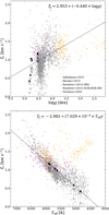 |
Fig. 1. ξt − log g (top panel) and ξt − Teff (bottom panel) correlations for the literature data, which are FGK dwarf stars of Adibekyan et al. (2012, grey triangles), FG dwarf stars of Bensby et al. (2014, grey circles) main-sequence to horizontal-branch stars of Roederer et al. (2014, grey and orange squares), and main-sequence stars of Hawkins et al. (2020, magenta squares). The dashed lines represent the least-squares fit of the data excluding non-main-sequence stars of Roederer et al. (2014) and stars with Teff < 5000 K of Adibekyan et al. (2012) and Bensby et al. (2014). The ξt has a better correlation with Teff than log g. Black circles are our target stars with ξt values obtained from Eq. (3). Open triangles and squares shows different ξt values estimated using the equations of Boeche & Grebel (2016) and Mashonkina et al. (2017), respectively. |
The ξt for our targets were then calculated from the Teff, which shows a better correlation with ξt than log g. In addition, we compared the obtained ξt values to those estimated using the relations of Boeche & Grebel (2016) and Mashonkina et al. (2017) in Table 2 and Fig. 1. Although our values are somewhat higher than the others, the difference in [Fe/H] by varying ξt by these typical deviations is smaller than 0.05 dex for each star.
Microturbulence velocity estimated using different equations.
We first estimated [Fe/H] from equivalent widths (EWs) of Fe lines with the Teff, log g, and ξt derived above. Then we iteratively performed the above procedures with the obtained [Fe/H] as the input value in the estimation of Teff until the newly estimated [Fe/H] was the same as the input value.
The finally obtained atmosphere parameters yield a balance of the Fe-abundance with excitation potential, but an equilibrium with reduced EW could not be reached. Although we attempted to derive spectroscopic log g for the sample stars from the ionisation equilibrium between Fe I and Fe II, we did not employ this value due to the high uncertainty on the EW measurements of Fe II lines. For ξt, we could not derive realistic values to reduce the trend between abundance and reduced EW at given Teff and log g. We also note that Teff values derived from (V − Ks) colour using the equation and coefficients of González Hernández & Bonifacio (2009) differ by up to 350 K from those using (BP − RP) colour. These discrepancies lead to a difference of up to 0.2 dex in [Fe/H] for each star. In this study, we employed the Gaia (BP − RP) colour to estimate Teff, based on their precise photometry. Our sample stars are plotted in a Kiel diagram in Fig. 2, and their atmospheric parameters are listed in Table 3.
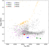 |
Fig. 2. Our wide binary samples and their location on a Kiel diagram, together with literature data as in Fig. 1. The WB1 (blue) and WB3 (red) pairs show very similar effective temperature and surface gravity between the component stars (ΔTeff ≤ 75 K; Δlog g ≤ 0.02 dex), while WB2 (green) has a larger difference in the effective temperature (ΔTeff = 229 K). |
Heliocentric velocities and atmospheric parameters.
3.2. Chemical abundance analysis
For spectroscopic abundance analysis, we applied model atmospheres interpolated from the ATLAS9 grid with α-enhanced opacity distributions (AODFNEW) by Castelli et al. (2003). The chemical abundances were determined using the 2017 version of the local thermodynamic equilibrium (LTE) code MOOG (Sneden 1973). We used the abfind driver of MOOG to derive Fe, Na, Si, Ca, Sc, Ti, V, Cr, Mn, Co, Ni, Cu, Zn, Y, Zr, and Ba abundances from the EWs of absorption lines, while the Mg abundance was obtained from spectrum synthesis using the MOOG synth driver. The EWs were measured by fitting single or multiple Gaussian profiles to isolated and blended lines with the semi-automatic code developed by Johnson et al. (2014). Table 4 presents the line list used in this work, which is based on that of Koch & McWilliam (2014). Hyperfine splitting was accounted for elements in which the splitting is significant (see the notes in Table 5). We note, however, that EWs of several lines within our spectral coverage for other elements, such as Al and Eu, could not be measured because the S/N was insufficient. The chemical abundances for each element, their line-to-line scatter (σ), and the number of lines used (N) are listed in Table 5 in terms of [X/H], adopting the solar abundance of Asplund et al. (2009).
Line list.
Chemical abundance results.
Systematic error due to the uncertainty in the atmosphere parameters.
3.3. Error analysis
To obtain an estimate for the statistical error on the abundance ratios, we list in Table 5 the line-to-line scatter and the number of lines we used for each element. Next, we estimated the systematic errors of the chemical abundance measurements, which can be caused by uncertainties in atmospheric parameters, through comparison with abundances measured from altered atmosphere models. For this purpose, we interpolated eight atmosphere models with different atmosphere parameters varied by the typical uncertainty of our samples from the finally determined values (ΔTeff = ±65 K, Δlog g = ±0.1 dex, Δ[Fe/H] = ±0.17 dex, and Δξt = ±0.13 km s−1), and another model calculated using scaled-solar opacity distribution (ODFNEW).
The above uncertainties were computed by Monte Carlo sampling accounting for the errors on each input variable in the estimation. We first took the uncertainty in [Fe/H] from the standard deviation of the line-by-line Fe abundance measurements (see Table 5). The uncertainty in Teff was estimated, taking the above uncertainty in [Fe/H], magnitude error of Gaia DR2, and the dispersion in the empirical calibration of Mucciarelli & Bellazzini (2020) into account. In the same manner, we estimated uncertainties in log g and ξt based on the uncertainties of stellar mass (±0.2 M⊙), distance, magnitude, Teff, and fitting error of Eq. (3). Abundances were then re-derived with these altered models for all sample stars, and the systematic errors for each element depending on each parameter are listed in Table 6, averaged over all stars. The total systematic uncertainty is calculated to be the squared sum of all contributions, which should be seen as an upper limit owing to the covariances between the stellar parameters, however (e.g., McWilliam et al. 1995).
In addition, in order to examine the non-LTE effects on the determination of the abundances, we estimated the corrections for lines with available data based on Bergemann et al. (2012, 2013, 2017) 3. The average effects of non-LTE for Fe, Mg, Si, Ca, Ti, Cr, Mn, and Co elements are also given in Table 6, although these corrections were not applied to the interpretation of our spectroscopic results for the comparison with literature data (see Sect. 4.2). The non-LTE effects for Fe, Mg, Si, and Ca are negligible compared to the systematic errors, while those for Ti, Cr, Mn, and Co are somewhat large.
4. Abundance results
4.1. Chemical homogeneity of wide binaries
For comparison, Fig. 3 shows observed spectra of components in each wide binary pair. The stars of WB1 and WB2 have remarkably similar spectral features in the region of Fe, Mg, Ca, and Hα absorption lines, suggesting a similar chemical composition of co-moving stars. In the case of WB3, however, the component WB3b has stronger absorption lines for these elements than WB3a. It is intriguing that the WB3 pair shares similar abundances, in spite of the different shapes of parts of the spectra (see also Table 5). In particular, the stronger Hα absorption of WB3b is distinct and may indicate that WB3b is an unresolved binary itself, so that the continuum is falsified or the Hα line would be affected by a hot dwarf companion. If confirmed, the WB3 would be a good example for an emergence of wide binaries from higher-order multiplicity (e.g., Tokovinin 2014; Halbwachs et al. 2017).
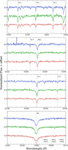 |
Fig. 3. Continuum-normalised spectra of stars showing several Fe, Mg, Ca, and Hα lines. The spectra of the components in WB1 and WB2 are almost identical in these spectral ranges. However, those for WB3 show differences in the strength of absorption lines, where WB3b has systematically stronger absorption lines. |
Our results show that the stars in each wide binary pair share very similar chemical abundances for all pairs we observed from our spectroscopic analysis (see Fig. 4). In the case of [Fe/H], the differences between the component stars are only 0.003, 0.015, and 0.025 dex for WB1, WB2, and WB3, respectively, which is much smaller than the systematic uncertainty of 0.1 dex and the statistical error of ∼0.02 dex (taken as σ/ ; Table 5). The identical metallicity of the wide binary components, as well as close proper motion and line-of-sight velocity, therefore strongly support the hypothesis that our sample stars are indeed wide binary pairs and not randomly co-moving stars. The marginal variations of [Fe/H] in each wide binary are comparable to those found in the literature (e.g., Desidera et al. 2004, 2006; Andrews et al. 2018; Hawkins et al. 2020).
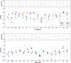 |
Fig. 4. [X/H] (upper) and [X/Fe] (lower) abundance ratios of wide binary stars and their differences between component stars of each wide binary (blue for WB1, green for WB2, and red for WB3). Dotted lines in the Δ[X/Y] plots denote the value of 0.0 and 0.3 dex, and the error bars indicate the 1σ statistical error. The differences in abundance between component stars are similarly small in the [X/H] and [X/Fe] abundance ratios. |
Our wide binaries are placed on the metal-poor side compared to previously reported wide binaries. The mean values of [Fe/H] are −1.16, −1.42, and −0.79 dex for WB1, WB2, and WB3, respectively, while the majority of spectroscopically confirmed wide binaries in the literature are within the metallicity span of −1.0 < [Fe/H] < +0.5 (e.g., Hwang et al. 2021). This does not come as a surprise, however, because our wide binary samples can be dynamically associated with the Milky Way halo and have explicitly been selected as such, whereas, for example, those of Andrews et al. (2018) and Hawkins et al. (2020) are associated with the Galactic disk. On the other hand, Hwang et al. (2021) have shown that the wide binary fraction is strongly dependent on metallicity, and it decreases with decreasing metallicity from [Fe/H] of 0.0 dex. Therefore metal-poor wide binaries ([Fe/H] < −1.0 dex) are expected to become extremely rare. We note that this metallicity dependence is mainly based on disk stars, and Hwang et al. (2021) claimed multiple formation channels of wide binaries depending on their metallicity. In this regard, the WB2 pair with [Fe/H] of −1.42 dex can provide an important and unusual opportunity to study the nature of metal-poor wide binaries in the halo.
Figure 4 presents the chemical abundance ratios for each element determined in this study in terms of [X/H] and [X/Fe], together with the differences between the component stars of wide binaries, Δ[X/Y]. Typically, the differences in abundances between either component are less than 0.1 dex, with some exceptions, such as the Si abundance of WB1 at the highest 0.25 dex level, probably due to the large line-to-line abundance variation (see Table 5 and Fig. 4). The Mg, Ca, and Ba abundances, for example, which have been derived from prominent and well-determined absorption lines, are highly consistent in every wide binary pair (Δ ≲ 0.05 dex). In addition, we could not find a peculiar chemical difference pattern between specific elements in our sample wide binaries. It therefore appears that the stars within any given wide binary share the same chemical composition, indicating that they have formed in the same environment. These chemical homogeneities of wide binary in various elements are comparable to what Andrews et al. (2018) and Hawkins et al. (2020) reported, while the discrepancies are somewhat larger than those seen in Hawkins et al. (2020). As described above, this is probably because of the larger uncertainties of our abundance measurement due to the lower S/N (∼25 per pixel) compared to that of (2020, S/N ∼ 105 per pixel).
4.2. Chemodynamical tagging
Chemical tagging is one of the best ways to trace the origin of stars (Freeman & Bland-Hawthorn 2002). This technique is widely employed in Galactic archaeology when extensive spectroscopic observations are available. In particular, numerous stellar streams and substructures, such as Gaia-Enceladus and Sequoia, have been revealed and characterised in the Milky Way through recent chemodynamical studies (e.g., Helmi et al. 2018; Myeong et al. 2019; Ji et al. 2020; Horta et al. 2021; Koch-Hansen et al. 2021; Prudil et al. 2021). In this vein, we compared the chemical and dynamical properties of our wide binaries with Galactic field stars to investigate their origin.
In Fig. 5 we plot the abundances of each α-element (Mg, Si, and Ca), their average, and Ti for our sample stars in comparison with Galactic bulge, disks, and halo stars obtained from multiple literature sources (see caption for details). Interestingly, the WB2 pair shows lower α-element abundances than the field stars within a similar metallicity region, in contrast to the other two pairs that closely follow their underlying the Milky Way halo environment. We note that the Si abundance of WB2ab stars could not be measured due to contamination by noise in the Si absorption lines. The large discrepancy in the Si abundance of the WB1 pair might also be affected by the large measurement error of WB1a (see Table 5 and Fig. 4). The plot of the average α-element abundance more clearly indicates the [α/Fe] depletion of the WB2 pair. The [α/Fe] abundances are 0.27/0.35 dex for WB1a/b, 0.24/0.18 dex for WB2a/b, and 0.20/0.27 dex for WB3a/b. The abundance pattern of WB2 we derived is consistent with the earlier studies by King (1997), Chen & Zhao (2006), Chen et al. (2014), and Reggiani & Meléndez (2018). These authors measured chemical abundances of this wide binary pair and reported [Fe/H] = −1.47/−1.53 dex (King 1997) and −1.43/−1.39 dex (Reggiani & Meléndez 2018) for WB2a (≡HD 134439)/WB2b (≡HD 134440), respectively, with an average [α/Fe] of ∼0.03 dex. This low α-element abundance has already been interpreted as evidence of an accretion origin in both studies. We note that the lower [α/Fe] abundances of previous studies compared to ours are due to the significant depletion of [Mg/Fe], which is not shown in this study.
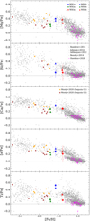 |
Fig. 5. Chemical abundance ratios of wide binaries for individual and average α-elements (Mg, Si, and Ca), and Ti, together with field stars in the Milky Way bulge (Johnson et al. 2014), disk (Adibekyan et al. 2012; Bensby et al. 2014), and halo (Adibekyan et al. 2012; Roederer et al. 2014). We also plot wide binaries in the disk (magenta squares: Hawkins et al. 2020) and halo stars also associated with the Sequoia (brown and yellow stars: Stephens & Boesgaard 2002; Monty et al. 2020). The horizontal dashed line indicates the solar level. It is interesting that the WB2 pair and the Sequoia G2 stars are commonly depleted in α-elements compared to the general trend of field stars. |
The low [α/Fe] abundance ratio at a given [Fe/H] is an important chemical signature of stars that accreted from dwarf galaxies due to the low star-forming efficiencies of these low-mass systems (see e.g., Tinsley 1979; Matteucci & Brocato 1990; Venn et al. 2004; Nissen & Schuster 2010; Hendricks et al. 2014; Hughes et al. 2020; Reichert et al. 2020). It is therefore likely that stars of WB2 were formed in a dwarf galaxy environment and then accreted into the Milky Way halo, as already conjectured by King (1997). Furthermore, the α-element abundances of WB2 follow the trend of the Sequoia G2 stars defined by Monty et al. (2020). The Sequoia accretion event has been identified by Myeong et al. (2019) from the bulk of the high-energy retrograde stars and globular clusters in the halo (see also Koch & Côté 2019; Massari et al. 2019; Villanova et al. 2019). The progenitor of Sequoia, with a predicted total mass between ∼108 M⊙ (Koppelman et al. 2019) and ∼1010 M⊙ (Myeong et al. 2019), was probably accreted onto the Milky Way 9–11 Gyr ago. More recently, Monty et al. (2020) re-observed stars of the Stephens & Boesgaard (2002) sample and found that a number of stars are dynamically coincident with the Gaia-Sausage and Sequoia events, which were not known features in 2002. They also reported that stars originating from Sequoia could be divided into two groups, G1 and G2, with slightly different orbital energy and α-element abundance patterns (see the yellow and brown stars in Figs. 5–7).
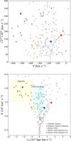 |
Fig. 7. Toomre and E − LZ diagrams for our wide binary sample, globular clusters (grey squares), and stars from Monty et al. (2020, stars). Globular clusters associated with the Sequoia event are indicated as purple squares (Massari et al. 2019). The curved dashed line in the upper panel denotes a total velocity of 180 km s−1, which divides the halo and thick disk, and yellow and cyan background boxes in the lower panel indicate the dynamical domains of the Sequoia and Gaia-Enceladus, respectively, as defined by Massari et al. (2019). Although the selection criterion for the Sequoia event slightly varies depending on the literature (e.g., Koppelman et al. 2019; Myeong et al. 2019), the WB2 pair shows remarkably similar properties to the Sequoia stars and its globular clusters. |
Figure 6 shows chemical abundances ratios of Na, Cr, Ni, Y, and Ba for our sample and field stars. It appears that the abundances of Fe-peak elements (Sc, V, Cr, Mn, Co, Cu, and Zn) and neutron-capture elements (Y, Zr, and Ba) of WB2 are on the global trend of the Milky Way stars, while slightly depleted in Ni abundance. This is difficult to confidently assert for these elements, however, owing to the large measurement and systematic errors. Nevertheless, we conclude that the WB2 pair and the Sequoia G2 stars also have comparable abundance ratios of [Na/Fe], [Y/Fe] and [Ba/Fe] (see also Fig. 13 of Monty et al. 2020).
In order to further investigate the origin of WB2 and the binary sample, we estimated their orbital parameters, namely orbital energy (E) and angular momentum (L), of stars using the galpy package (Bovy 2015) with the Galactic potential of McMillan (2017). Figure 7 presents the dynamical properties of our sample stars on a Toomre diagram (upper panel) and in the E − LZ plane (lower panel). WB2 is located in a region that is remarkably similar to that of the Sequoia G2 stars, not only in the Toomre diagram, but also in the E − LZ diagram. In addition, the orbital parameters of WB2 are also comparable to those of globular clusters that have been suggested to be associated with the Sequoia event by Massari et al. (2019). The dynamical properties of WB2 as well as its low α-element abundances therefore strongly suggest that this wide binary originated from an accreted dwarf galaxy, specifically, the progenitor of Sequoia.
In contrast to WB2, we could not detect any obvious chemical nor dynamical peculiarities of the WB1 and WB3 binaries when compared to the Milky Way field stars. Although the orbital parameters of WB1 mildly overlap with the Gaia-Enceladus event in the E − LZ plane, stars of this binary pair do not show a low [α/Fe] abundance, which has been observed in the Gaia-Enceladus stars, however (see e.g. Fig. 4 of Koppelman et al. 2019).
5. Discussion
We confirm through spectroscopic observations that three wide pairs of common proper motion stars with high space velocities are indeed bound system, based on their common dynamical and chemical properties between the component stars. These stars are rare cases of wide binaries as metal-poor halo tracers (see e.g., Hwang et al. 2021). Our analysis demonstrates chemical homogeneity between their components, as is also seen in metal-rich wide binaries in the disks (e.g., Hawkins et al. 2020). This makes the chemical composition one of the global properties of a wide binary and suggests a common origin in a chemically similar environment.
Moreover, our study suggests that one of our wide binary pairs is associated with the Sequoia event. An accretion origin of the WB2 pair has long been suspected: King (1997) suggested chemical similarity of this wide binary with the globular clusters Rup 106 and Pal 12, which in turn are associated with the Magellanic Clouds. Reggiani & Meléndez (2018) claimed a link with dwarf spheroidal galaxies such as Fornax. In this study, we find that the WB2 is more likely related to the Sequoia event based on both chemical and dynamical properties. This pair provides a significant opportunity to examine not only the formation mechanism of wide binaries, but also the assembly process of the Milky Way halo. At first glance, the existence of this wide binary supports the formation scenario suggested by Peñarrubia (2021), which predicts that a large number of ultra-wide binaries with separations ≳0.1 pc arises from the disruption of low-mass systems, such as streams of globular clusters, over several Gyr. We note, however, that the physical separation of WB2 (s ∼ 0.04 pc) is smaller than those of Peñarrubia (2021, s > 0.1 pc), and the total mass of the Sequoia is likely much more massive (MSeq ∼ 1010 M⊙; Myeong et al. 2019) than the progenitors adopted in the simulations of Peñarrubia (2021).
On the other hand, within the framework of Kouwenhoven et al. (2010) and Moeckel & Clarke (2011), it is conceivable that both WB2 component stars were individually formed in a stellar cluster belonging to the Sequoia progenitor and were subsequently bound into a binary during the early dissolution phase of the cluster. If the WB2 components were already bound in the Sequoia progenitor either through the above process, the dynamical unfolding (Reipurth & Mikkola 2012), or the formation from adjacent stellar cores (Tokovinin 2017), it is significant to know whether the system can survive during the tidal disruption of the progenitor. Whether this is a likely scenario depends on the properties of the progenitor dwarf galaxy and the peak separation of the wide binary. The estimation in Appendix A suggests that wide binaries with a combined mass of 1 M⊙ and a semi-major axis < 1.4 pc will survive in the tidal field that disrupts dwarf galaxies with a half-light radius of ∼100 pc or larger. Thus, it seems a plausible scenario that the WB2 pair formed in the progenitor galaxy and was later accreted onto the Galactic halo, although detailed dynamical modelling of the Sequoia progenitor and its disruption in the Milky Way tidal field is necessary to explore this possibility further. In this regard, wide binaries may provide novel constraints on the hierarchical build up of the Milky Way halo.
A key remaining question is whether WB2 is a rare case or if a larger fraction of wide binaries can be associated with such Milky Way accretion events. Interestingly, another peculiar wide binary (G 112-43/44) associated with the Helmi streams (Helmi et al. 1999) has recently been reported by Nissen et al. (2021). This finding, along with ours, implies that more wide binaries related to accretion events are embedded in the Galactic halo. In particular, because the WB2 is only ∼30 pc away from the Sun, we can reasonably expect that many more similar cases are waiting to be discovered in the entire Milky Way. Although WB2 is currently located in the Galactic disk region, its metallicity and dynamical properties rather associate it with the Galactic halo. This is also in line with the finding of an increasing separation with the binary height above the plane (Sesar et al. 2008). Further searches for such wide binaries through chemodynamical studies will provide a novel opportunity to understand the formation of wide binaries and the assembly process of the Milky Way.
Acknowledgments
We thank the referee for a number of helpful suggestions. DL and AJKH gratefully acknowledges funding by the Deutsche Forschungsgemeinschaft (DFG, German Research Foundation) – Project-ID 138713538 – SFB 881 (“The Milky Way System”), subprojects A03, A05, A11. DL thanks Sree Oh for the consistent support.
References
- Adibekyan, V. Z., Sousa, S. G., Santos, N. C., et al. 2012, A&A, 545, A32 [NASA ADS] [CrossRef] [EDP Sciences] [Google Scholar]
- Aguado, D. S., Belokurov, V., Myeong, G. C., et al. 2021, ApJ, 908, L8 [NASA ADS] [CrossRef] [Google Scholar]
- Allen, C., Poveda, A., & Hernández-Alcántara, A. 2007, in Binary Stars as Critical Tools& Tests in Contemporary Astrophysics, eds. W. I. Hartkopf, P. Harmanec, & E. F. Guinan, 240, 405 [NASA ADS] [Google Scholar]
- Andrews, J. J., Chanamé, J., & Agüeros, M. A. 2017, MNRAS, 472, 675 [NASA ADS] [CrossRef] [Google Scholar]
- Andrews, J. J., Chanamé, J., & Agüeros, M. A. 2018, MNRAS, 473, 5393 [NASA ADS] [CrossRef] [Google Scholar]
- Asplund, M., Grevesse, N., Sauval, A. J., & Scott, P. 2009, ARA&A, 47, 481 [NASA ADS] [CrossRef] [Google Scholar]
- Bahcall, J. N., Hut, P., & Tremaine, S. 1985, ApJ, 290, 15 [NASA ADS] [CrossRef] [Google Scholar]
- Bensby, T., Feltzing, S., & Oey, M. S. 2014, A&A, 562, A71 [NASA ADS] [CrossRef] [EDP Sciences] [Google Scholar]
- Bergemann, M., Lind, K., Collet, R., Magic, Z., & Asplund, M. 2012, MNRAS, 427, 27 [Google Scholar]
- Bergemann, M., Kudritzki, R.-P., Würl, M., et al. 2013, ApJ, 764, 115 [NASA ADS] [CrossRef] [Google Scholar]
- Bergemann, M., Collet, R., Amarsi, A. M., et al. 2017, ApJ, 847, 15 [NASA ADS] [CrossRef] [Google Scholar]
- Boeche, C., & Grebel, E. K. 2016, A&A, 587, A2 [NASA ADS] [CrossRef] [EDP Sciences] [Google Scholar]
- Bovy, J. 2015, ApJS, 216, 29 [NASA ADS] [CrossRef] [Google Scholar]
- Casagrande, L., & VandenBerg, D. A. 2018, MNRAS, 479, L102 [NASA ADS] [CrossRef] [Google Scholar]
- Castelli, F., & Kurucz, R. L. 2003, Modelling of Stellar Atmospheres, eds. N. Piskunov, W. W. Weiss, & D. F. Gray, 210, A20 [Google Scholar]
- Chanamé, J., & Gould, A. 2004, ApJ, 601, 289 [CrossRef] [Google Scholar]
- Chen, Y. Q., & Zhao, G. 2006, MNRAS, 370, 2091 [NASA ADS] [CrossRef] [Google Scholar]
- Chen, Y., King, J. R., & Boesgaard, A. M. 2014, PASP, 126, 1010 [NASA ADS] [CrossRef] [Google Scholar]
- Coronado, J., Sepúlveda, M. P., Gould, A., & Chanamé, J. 2018, MNRAS, 480, 4302 [NASA ADS] [CrossRef] [Google Scholar]
- Desidera, S., Gratton, R. G., Scuderi, S., et al. 2004, A&A, 420, 683 [NASA ADS] [CrossRef] [EDP Sciences] [Google Scholar]
- Desidera, S., Gratton, R. G., Lucatello, S., & Claudi, R. U. 2006, A&A, 454, 581 [NASA ADS] [CrossRef] [EDP Sciences] [Google Scholar]
- El-Badry, K., & Rix, H.-W. 2018, MNRAS, 480, 4884 [Google Scholar]
- Elliott, P., & Bayo, A. 2016, MNRAS, 459, 4499 [NASA ADS] [CrossRef] [Google Scholar]
- Fernández-Trincado, J. G., Zamora, O., García-Hernández, D. A., et al. 2017, ApJ, 846, L2 [Google Scholar]
- Freeman, K., & Bland-Hawthorn, J. 2002, ARA&A, 40, 487 [Google Scholar]
- Gaia Collaboration (Brown, A. G. A., et al.) 2016, A&A, 595, A2 [NASA ADS] [CrossRef] [EDP Sciences] [Google Scholar]
- Gaia Collaboration (Brown, A. G. A., et al.) 2018, A&A, 616, A1 [NASA ADS] [CrossRef] [EDP Sciences] [Google Scholar]
- Gaia Collaboration (Brown, A. G. A., et al.) 2021, A&A, 649, A1 [NASA ADS] [CrossRef] [EDP Sciences] [Google Scholar]
- González Hernández, J. I., & Bonifacio, P. 2009, A&A, 497, 497 [Google Scholar]
- Green, G. M., Schlafly, E. F., Finkbeiner, D., et al. 2018, MNRAS, 478, 651 [Google Scholar]
- Halbwachs, J. L., Mayor, M., & Udry, S. 2017, MNRAS, 464, 4966 [NASA ADS] [CrossRef] [Google Scholar]
- Hanke, M., Hansen, C. J., Koch, A., & Grebel, E. K. 2018, A&A, 619, A134 [NASA ADS] [CrossRef] [EDP Sciences] [Google Scholar]
- Hartman, Z. D., & Lépine, S. 2020, ApJS, 247, 66 [NASA ADS] [CrossRef] [Google Scholar]
- Hawkins, K., Lucey, M., Ting, Y.-S., et al. 2020, MNRAS, 492, 1164 [NASA ADS] [CrossRef] [Google Scholar]
- Helmi, A., White, S. D. M., de Zeeuw, P. T., & Zhao, H. 1999, Nature, 402, 53 [Google Scholar]
- Helmi, A., Babusiaux, C., Koppelman, H. H., et al. 2018, Nature, 563, 85 [Google Scholar]
- Hendricks, B., Koch, A., Lanfranchi, G. A., et al. 2014, ApJ, 785, 102 [NASA ADS] [CrossRef] [Google Scholar]
- Horta, D., Schiavon, R. P., Mackereth, J. T., et al. 2021, MNRAS, 500, 1385 [Google Scholar]
- Hughes, M. E., Pfeffer, J. L., Martig, M., et al. 2020, MNRAS, 491, 4012 [NASA ADS] [CrossRef] [Google Scholar]
- Hwang, H.-C., Ting, Y.-S., Schlaufman, K. C., Zakamska, N. L., & Wyse, R. F. G. 2021, MNRAS, 501, 4329 [NASA ADS] [CrossRef] [Google Scholar]
- Ji, A. P., Li, T. S., Hansen, T. T., et al. 2020, AJ, 160, 181 [NASA ADS] [CrossRef] [Google Scholar]
- Jiménez-Esteban, F. M., Solano, E., & Rodrigo, C. 2019, AJ, 157, 78 [Google Scholar]
- Johnson, C. I., Rich, R. M., Kobayashi, C., Kunder, A., & Koch, A. 2014, AJ, 148, 67 [Google Scholar]
- Kelson, D. D. 2003, PASP, 115, 688 [NASA ADS] [CrossRef] [Google Scholar]
- King, I. 1962, AJ, 67, 471 [Google Scholar]
- King, J. R. 1997, AJ, 113, 2302 [NASA ADS] [CrossRef] [Google Scholar]
- Koch, A., & Côté, P. 2019, A&A, 632, A55 [NASA ADS] [CrossRef] [EDP Sciences] [Google Scholar]
- Koch, A., & McWilliam, A. 2014, A&A, 565, A23 [NASA ADS] [CrossRef] [EDP Sciences] [Google Scholar]
- Koch, A., Grebel, E. K., & Martell, S. L. 2019, A&A, 625, A75 [NASA ADS] [CrossRef] [EDP Sciences] [Google Scholar]
- Koch-Hansen, A. J., Hansen, C. J., & McWilliam, A. 2021, A&A, 653, A2 [NASA ADS] [CrossRef] [EDP Sciences] [Google Scholar]
- Koppelman, H. H., Helmi, A., Massari, D., Price-Whelan, A. M., & Starkenburg, T. K. 2019, A&A, 631, L9 [NASA ADS] [CrossRef] [EDP Sciences] [Google Scholar]
- Kouwenhoven, M. B. N., Goodwin, S. P., Parker, R. J., et al. 2010, MNRAS, 404, 1835 [NASA ADS] [Google Scholar]
- Kunder, A., Kordopatis, G., Steinmetz, M., et al. 2017, AJ, 153, 75 [Google Scholar]
- Lee, J.-E., Lee, S., Dunham, M. M., et al. 2017, Nat. Astron., 1, 0172 [NASA ADS] [CrossRef] [Google Scholar]
- Lépine, S., & Gaidos, E. 2011, AJ, 142, 138 [Google Scholar]
- Lépine, S., & Shara, M. M. 2005, AJ, 129, 1483 [Google Scholar]
- Lim, D., Lee, Y.-W., Koch, A., et al. 2021, ApJ, 907, 47 [NASA ADS] [CrossRef] [Google Scholar]
- Luo, A. L., Zhao, Y.-H., Zhao, G., et al. 2015, Res. Astron. Astrophys., 15, 1095 [Google Scholar]
- Marshall, J. L., Burles, S., Thompson, I. B., et al. 2008, in Ground-based and Airborne Instrumentation for Astronomy II, eds. I. S. McLean, & M. M. Casali, SPIE Conf. Ser., 7014, 701454 [NASA ADS] [Google Scholar]
- Mashonkina, L., Jablonka, P., Pakhomov, Y., Sitnova, T., & North, P. 2017, A&A, 604, A129 [NASA ADS] [CrossRef] [EDP Sciences] [Google Scholar]
- Massari, D., Koppelman, H. H., & Helmi, A. 2019, A&A, 630, L4 [NASA ADS] [CrossRef] [EDP Sciences] [Google Scholar]
- Matteucci, F., & Brocato, E. 1990, ApJ, 365, 539 [CrossRef] [Google Scholar]
- McMillan, P. J. 2017, MNRAS, 465, 76 [NASA ADS] [CrossRef] [Google Scholar]
- McWilliam, A., Preston, G. W., Sneden, C., & Searle, L. 1995, AJ, 109, 2757 [Google Scholar]
- McWilliam, A., Rich, R. M., & Smecker-Hane, T. A. 2003, ApJ, 592, L21 [NASA ADS] [CrossRef] [Google Scholar]
- Moeckel, N., & Clarke, C. J. 2011, MNRAS, 415, 1179 [NASA ADS] [CrossRef] [Google Scholar]
- Monroy-Rodríguez, M. A., & Allen, C. 2014, ApJ, 790, 159 [CrossRef] [Google Scholar]
- Monty, S., Venn, K. A., Lane, J. M. M., Lokhorst, D., & Yong, D. 2020, MNRAS, 497, 1236 [NASA ADS] [CrossRef] [Google Scholar]
- Mucciarelli, A., & Bellazzini, M. 2020, Res. Notes Am. Astron. Soc., 4, 52 [Google Scholar]
- Myeong, G. C., Vasiliev, E., Iorio, G., Evans, N. W., & Belokurov, V. 2019, MNRAS, 488, 1235 [Google Scholar]
- Nissen, P. E., & Schuster, W. J. 2010, A&A, 511, L10 [NASA ADS] [CrossRef] [EDP Sciences] [Google Scholar]
- Nissen, P. E., Silva-Cabrera, J. S., & Schuster, W. J. 2021, A&A, 651, A57 [NASA ADS] [CrossRef] [EDP Sciences] [Google Scholar]
- Palacios, A., Gebran, M., Josselin, E., et al. 2010, A&A, 516, A13 [NASA ADS] [CrossRef] [EDP Sciences] [Google Scholar]
- Peñarrubia, J. 2021, MNRAS, 501, 3670 [Google Scholar]
- Prudil, Z., Hanke, M., Lemasle, B., et al. 2021, A&A, 648, A78 [NASA ADS] [CrossRef] [EDP Sciences] [Google Scholar]
- Quinn, D. P., Wilkinson, M. I., Irwin, M. J., et al. 2009, MNRAS, 396, L11 [NASA ADS] [CrossRef] [Google Scholar]
- Quinn, D. P., Wilkinson, M. I., Irwin, M. J., et al. 2010, in Binaries– Key to Comprehension of the Universe, eds. A. Prša, & M. Zejda, ASP Conf. Ser., 435, 453 [Google Scholar]
- Reggiani, H., & Meléndez, J. 2018, MNRAS, 475, 3502 [NASA ADS] [CrossRef] [Google Scholar]
- Reichert, M., Hansen, C. J., Hanke, M., et al. 2020, A&A, 641, A127 [NASA ADS] [CrossRef] [EDP Sciences] [Google Scholar]
- Reipurth, B., & Mikkola, S. 2012, Nature, 492, 221 [NASA ADS] [CrossRef] [Google Scholar]
- Roederer, I. U., Preston, G. W., Thompson, I. B., et al. 2014, AJ, 147, 136 [Google Scholar]
- Sesar, B., Ivezić, Ž., & Jurić, M. 2008, ApJ, 689, 1244 [NASA ADS] [CrossRef] [Google Scholar]
- Sneden, C. A. 1973, Ph.D. Thesis, The University of Texas at Austin [Google Scholar]
- Stephens, A., & Boesgaard, A. M. 2002, AJ, 123, 1647 [NASA ADS] [CrossRef] [Google Scholar]
- Telting, J. H., Avila, G., Buchhave, L., et al. 2014, Astron. Nachr., 335, 41 [Google Scholar]
- Tian, H.-J., El-Badry, K., Rix, H.-W., & Gould, A. 2020, ApJS, 246, 4 [Google Scholar]
- Tinsley, B. M. 1979, ApJ, 229, 1046 [Google Scholar]
- Tokovinin, A. 2014, AJ, 147, 87 [CrossRef] [Google Scholar]
- Tokovinin, A. 2017, MNRAS, 468, 3461 [NASA ADS] [CrossRef] [Google Scholar]
- Venn, K. A., Irwin, M., Shetrone, M. D., et al. 2004, AJ, 128, 1177 [NASA ADS] [CrossRef] [Google Scholar]
- Villanova, S., Monaco, L., Geisler, D., et al. 2019, ApJ, 882, 174 [NASA ADS] [CrossRef] [Google Scholar]
- Walker, M. G., Mateo, M., Olszewski, E. W., et al. 2009, ApJ, 704, 1274 [Google Scholar]
- Yoo, J., Chanamé, J., & Gould, A. 2004, ApJ, 601, 311 [NASA ADS] [CrossRef] [Google Scholar]
Appendix A: Survival or disruption of wide binary during the accretion event
In the following, we estimate whether a wide binary in a progenitor dwarf galaxy could survive during the accretion of the system into the Milky Way. The tidal radius of a dwarf satellite galaxy can be estimated as follows (King 1962):
where rt, Msat, and D are the tidal radius, mass, and Galactocentric distance of the dwarf satellite galaxy, and MMW is the mass of the Milky Way. The satellite will lose its stars when rt < 2rhalf, sat, where rhalf, sat is the half-light radius of the satellite. In the same manner, the binary in the satellite will be disrupted if the tidal radius is
where MWB and a are the mass and semi-major axis of binary. Because the binary would experience the same tidal field as the affiliated dwarf galaxy, these two equations are combined based on the common terms. We further assume that the tidal interaction of the binary with the potential of the satellite galaxy is negligible relative to that of the Milky Way. Thus, we obtain the following condition for the disruption of a binary to occur:
In addition, Walker et al. (2009) found a tight correlation between mass and half-light radius of the dwarf spheroidal galaxy as follows:

By employing Equation (A.4), Equation (A.3) can be converted into
This equation implies that if we assume the dwarf satellite galaxy of rhalf > 100 pc, wide binaries of 1 M⊙ with a > 1.4 pc will be disrupted upon accretion of the host system onto the Milky Way. In other words, wide binaries with a < 1.4 pc could survive in the tidal field that disrupts the progenitor dwarf satellite galaxy. The condition of the semi-major axis for survival or disruption of wide binary increases with increasing mass of the binary and the half-light radius of the progenitor.
Appendix B: Further observations of binaries and non-binaries
An earlier set of observations was acquired at lower spectral resolution and the data were of lower quality, allowing for a mere kinematic study. We briefly describe these data and list the radial velocities so that these candidates can be in- and excluded in future statistical analyses, for instance in the assessment of the clumpy dark matter distribution in the halo (e.g. Chanamé & Gould 2004; Quinn et al. 2009).
A.1. MIKE spectra
We observed two further binary pairs with the Magellan Inamori Kyocera Echelle (MIKE) spectrograph at the 6.5 m Magellan2/Clay Telescope in November 2008 and July 2009 using a slit width of 0.7″ and a binning of 2×2 CCD pixels in the spatial and spectral dimensions. For details of the data and their reduction, we refer to Quinn et al. (2009). While taken at high resolution (R∼40000), the spectra are hampered by unfortunately low S/N (< 20 per pixel at Hα) that only permitted radial velocity measurements, but not the derivation of chemical abundance ratios.
A.2. MagE spectra
During three nights in July 2009, we acquired spectra of four further wide binary candidate pairs with the Magellan Echellette (MagE) spectrograph (Marshall et al. 2008). Our target selection for this campaign was based on the same criteria as outlined in Section 2.1. MagE yields a much lower spectral resolution than MIKE, and we integrated for considerably shorter times and will primarily focus on velocity measurements for assessing the binarity of the stars from these data. In practice, MagE was used with its standard setting, that is, with a 1″ slit and a binning of 1×1 in spectral and spatial directions. This yielded a resolving power of R∼4100.
The data were reduced with the IDL-based pipeline kindly provided by G. Becker. This pipeline is largely built on the same principles and techniques as are used within the MIKE pipeline (Kelson 2003). As before, the basic reduction steps comprise flatfield corrections using both Xe-flash lamp exposures and dome flats, wavelength calibration through Th-Ar lamps that were taken between each pair of science exposures, and optimal extraction and sky subtraction.
A.3. FIES spectra
Two further pairs have been targeted with the FIES instrument within the same campaign that provided the sample we analysed here; accordingly, the observation and reduction procedures are identical to those outlined in Section 2. As they show very different radial velocities, these stars have not been incorporated in our above chemodynamic analysis.
A.4. Radial velocities and non-binarity
Using IRAF’s fxcor task, we cross-correlated the spectra against a synthetic template with stellar parameters similar to the target stars. The results are listed in Table B.1.
Details of the binary candidates and non-binaries that we did not use.
Out of the 11 candidate pairs that we observed as part of our campaign, 3 (i.e. 27%) could be refuted as physically bound systems based on their significantly (≫10σ) different radial velocities. Quinn et al. (2009) have impressively demonstrated the sensitivity of the predicted mass range of the clumpy dark matter in the halo in the form of MACHOs to the widest-separation binaries. In particular, Quinn et al. (2010) argued that the in- or exclusion of even a single wide binary pair at very large angular separation has dramatic consequences for the conclusions that can be drawn; the removal of a pair at the 1 pc level erases the constraints on the MACHO models at the 95% level. However, given the availability of systematic, large samples (e.g. Monroy-Rodríguez & Allen 2014; Coronado et al. 2018; Hartman & Lépine 2020) and the small size of our preselected sample, we defer a reanalysis of the statistics following Quinn et al. (2009) to a future work.
All Tables
All Figures
|
Fig. 1. ξt − log g (top panel) and ξt − Teff (bottom panel) correlations for the literature data, which are FGK dwarf stars of Adibekyan et al. (2012, grey triangles), FG dwarf stars of Bensby et al. (2014, grey circles) main-sequence to horizontal-branch stars of Roederer et al. (2014, grey and orange squares), and main-sequence stars of Hawkins et al. (2020, magenta squares). The dashed lines represent the least-squares fit of the data excluding non-main-sequence stars of Roederer et al. (2014) and stars with Teff < 5000 K of Adibekyan et al. (2012) and Bensby et al. (2014). The ξt has a better correlation with Teff than log g. Black circles are our target stars with ξt values obtained from Eq. (3). Open triangles and squares shows different ξt values estimated using the equations of Boeche & Grebel (2016) and Mashonkina et al. (2017), respectively. |
| In the text | |
|
Fig. 2. Our wide binary samples and their location on a Kiel diagram, together with literature data as in Fig. 1. The WB1 (blue) and WB3 (red) pairs show very similar effective temperature and surface gravity between the component stars (ΔTeff ≤ 75 K; Δlog g ≤ 0.02 dex), while WB2 (green) has a larger difference in the effective temperature (ΔTeff = 229 K). |
| In the text | |
|
Fig. 3. Continuum-normalised spectra of stars showing several Fe, Mg, Ca, and Hα lines. The spectra of the components in WB1 and WB2 are almost identical in these spectral ranges. However, those for WB3 show differences in the strength of absorption lines, where WB3b has systematically stronger absorption lines. |
| In the text | |
|
Fig. 4. [X/H] (upper) and [X/Fe] (lower) abundance ratios of wide binary stars and their differences between component stars of each wide binary (blue for WB1, green for WB2, and red for WB3). Dotted lines in the Δ[X/Y] plots denote the value of 0.0 and 0.3 dex, and the error bars indicate the 1σ statistical error. The differences in abundance between component stars are similarly small in the [X/H] and [X/Fe] abundance ratios. |
| In the text | |
|
Fig. 5. Chemical abundance ratios of wide binaries for individual and average α-elements (Mg, Si, and Ca), and Ti, together with field stars in the Milky Way bulge (Johnson et al. 2014), disk (Adibekyan et al. 2012; Bensby et al. 2014), and halo (Adibekyan et al. 2012; Roederer et al. 2014). We also plot wide binaries in the disk (magenta squares: Hawkins et al. 2020) and halo stars also associated with the Sequoia (brown and yellow stars: Stephens & Boesgaard 2002; Monty et al. 2020). The horizontal dashed line indicates the solar level. It is interesting that the WB2 pair and the Sequoia G2 stars are commonly depleted in α-elements compared to the general trend of field stars. |
| In the text | |
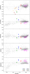 |
Fig. 6. Same as Fig. 5, but for Na, Cr, Ni, Y, and Ba. |
| In the text | |
|
Fig. 7. Toomre and E − LZ diagrams for our wide binary sample, globular clusters (grey squares), and stars from Monty et al. (2020, stars). Globular clusters associated with the Sequoia event are indicated as purple squares (Massari et al. 2019). The curved dashed line in the upper panel denotes a total velocity of 180 km s−1, which divides the halo and thick disk, and yellow and cyan background boxes in the lower panel indicate the dynamical domains of the Sequoia and Gaia-Enceladus, respectively, as defined by Massari et al. (2019). Although the selection criterion for the Sequoia event slightly varies depending on the literature (e.g., Koppelman et al. 2019; Myeong et al. 2019), the WB2 pair shows remarkably similar properties to the Sequoia stars and its globular clusters. |
| In the text | |
Current usage metrics show cumulative count of Article Views (full-text article views including HTML views, PDF and ePub downloads, according to the available data) and Abstracts Views on Vision4Press platform.
Data correspond to usage on the plateform after 2015. The current usage metrics is available 48-96 hours after online publication and is updated daily on week days.
Initial download of the metrics may take a while.