| Issue |
A&A
Volume 655, November 2021
|
|
|---|---|---|
| Article Number | A53 | |
| Number of page(s) | 19 | |
| Section | Numerical methods and codes | |
| DOI | https://doi.org/10.1051/0004-6361/202141392 | |
| Published online | 17 November 2021 | |
Spectral shape corrections for SDSS BOSS quasars
1
INAF, Osservatorio Astronomico di Trieste, Via G. B. Tiepolo 11, 34143 Trieste, Italy
e-mail: This email address is being protected from spambots. You need JavaScript enabled to view it.
2
Clare Hall, University of Cambridge, Herschel Road, Cambridge CB3 9AL, UK
3
AdServer Ltd, 37 Professora Popova Street, Saint-Petersburg 197022, Russia
Received:
26
May
2021
Accepted:
9
August
2021
Abstract
Modifications were made to the Sloan Digital Sky Survey’s Baryonic Oscillations Spectroscopic Survey (SDSS/BOSS) optical fibres assigned to quasar targets in order to improve the signal-to-noise ratio in the Ly-α forest. However, the consequence of these modifications is that quasars observed in this way require additional flux correction procedures in order to recover the correct spectral shapes. In this paper we describe such a procedure, based on the geometry of the problem, and other observational parameters. Applying several correction methods to four SDSS quasars with multiple observations permits a detailed verification of the relative performances of the different flux correction procedures. We contrast our method (which takes into account a wavelength-dependent seeing profile) with the BOSS pipeline approach (which does not). Our results provide independent confirmation that the geometric approach employed in the SDSS pipeline works well, although with room for improvement. By separating the contributions from four effects, we are able to quantify their relative importance. Most importantly, we demonstrate that wavelength dependence has a significant impact on the derived spectral shapes and thus should not be ignored.
Key words: instrumentation: spectrographs / cosmology: observations / quasars: absorption lines / intergalactic medium / surveys / techniques: spectroscopic
© ESO 2021
1. Introduction
Absorption by neutral hydrogen leaves a series of absorption lines imprinted on the spectra of distant quasars, known as the Ly-α forest (e.g. Lynds 1971; Sargent et al. 1980; Weymann et al. 1981; Rauch 1998). This gas traces the matter distribution on Gpc scales and can be used to study the distribution and evolution of baryons over cosmological timescales (e.g. Kim et al. 2002; Penton et al. 2004; Lehner et al. 2007; Zavarygin & Webb 2019). Large statistical samples of the Ly-α forest are therefore important tools for cosmological studies. The Baryonic Oscillations Spectroscopic Survey (BOSS, Ahn et al. 2012) and its extension eBOSS (Dawson et al. 2016), part of the Sloan Digital Sky Survey (SDSS, York et al. 2000), provide the largest available sample of medium-resolution quasar spectra.
BOSS quasar spectra (Dawson et al. 2013) are known to suffer from at least two systematic effects: the ‘Balmer problem’ and the ‘fibre offset problem’ (Lee et al. 2013). The Balmer problem arises from stellar absorption not being properly accounted for when flux calibrating the quasar spectra, such that the derived flux calibration correction function has residual stellar absorption features that can be transferred to the quasar spectra. The fibre offset problem for BOSS quasar spectra exists because quasars and photometric calibrating stars were fibre-centred at different central wavelengths. This was done in order to maximise the signal-to-noise ratio (S/N) in the Ly-α forest. However, neglecting to correct for it results in incorrect quasar spectral shapes (Lee et al. 2013). For this reason, a geometric procedure was implemented (Margala et al. 2016) to correct quasar spectral shapes.
Prior to seeing the comprehensive analysis of Margala et al. (2016), we had already developed a similar (but slightly simpler) method, which was being prepared for publication. Once the Margala procedure had been published, we saw little point in publishing our own, and shelved the work. However, during a more recent detailed analysis of Ly-α forest data to constrain cosmological isotropy (Zavarygin & Webb 2019), we discovered a systematic in SDSS BOSS spectra that emulates anisotropy and appears to be, at least in part, generated by the application of the fibre offset correction method of Margala et al. (2016). This motivated us to re-examine the issue, hence the present paper in which we present a new and independent geometric correction method. The method we introduce here and that of Margala adopt the same basic geometric approach. However, unlike ours (since some of the relevant technical data were not available to us), the Margala method includes corrections to account for a quasar’s plate position; that is, focal plane dependency. On the other hand, the Margala method assumes a constant seeing profile, whereas ours does not and instead allows for wavelength dependence.
The rest of this paper is structured as follows. In Sect. 2, we describe the geometry of the problem, the modifications made to the BOSS optical fibres assigned to quasars, and the mathematical model used to correct the fibre offset problem. We show that the effect of wavelength-dependant seeing is significant and must be taken into account. In Sect. 3, we define selection procedures to identify quasars with multiple exposures since these enable a direct test of how well the correction procedures work. The stringent and specific selection results in only four suitable quasars in the SDSS samples. The results of applying various correction procedures are described in Sect. 4. Section 5 discusses the findings of this study, and the appendices provide corresponding details for three quasars, with only one quasar being illustrated in the main text.
2. Fibre-offset geometry and corrections
2.1. The BOSS spectrograph
BOSS is a component of the SDSS-III survey (Eisenstein et al. 2011; Ahn et al. 2012). SDSS BOSS is conducted on a 2.5 m Sloan telescope (Gunn et al. 2006) at Apache Point Observatory in New Mexico, providing the spectra of ∼1.5 million luminous red galaxies up to z = 0.7 and ∼150 000 quasar spectra at z > 2 (Dawson et al. 2013). Quasar targets for the spectroscopic survey are selected based on the object colours, derived from earlier photometric imaging (see Ross et al. 2012 for details on how quasars are selected for spectroscopy). The thirteenth BOSS data release (DR13) contains more than 294 000 medium-resolution (R = λ/Δλ ≈ 1500 − 2500, where Δλ is the full width at half maximum of the one-dimensional point spread function) quasar spectra, covering more than 10 400 deg2 (Alam et al. 2015).
The BOSS spectra are obtained using twin spectrographs covering a wavelength range of ∼3000 − 11 000 Å. The spectrographs are fed by 1000 optical fibres (500 per spectrograph), each sub-tending 2″ on the sky. Further details about the spectrograph design can be found in Smee et al. (2013). Observations were designed to maximise the fraction of BOSS scientific targets assigned a fibre. A maximum of 900 fibres were assigned to scientific targets such as quasars. The remainder were reserved for calibration stars and sky background observations (Dawson et al. 2013).
2.2. The fibre offset problem
Atmospheric differential refraction will cause the centre of the quasar seeing profile to vary with wavelength and altitude on the sky. In order to obtain more precise data on the Ly-α forest (i.e. to improve the S/N at wavelengths λ ≲ 4000 Å; Dawson et al. 2013; Lee et al. 2013), the mechanics of attaching the optical fibres used for quasar observations to BOSS plate positions was modified in two ways: (1) thin wafers of sizes 175 − 300 μm (the size of the wafer depends on the distance of the fibre plug to the plate centre) were attached to the plug holes to provide an offset to the focal plane along the z-axis (i.e. towards the target); (2) the positions of the fibres were also offset by up to ∼0.5″ in the focal plane (i.e. along the x- and y-axes) in order to maximise the light entering the fibre. These fibre adjustments were thus both lateral and axial and designed such that the target image and fibre centre coincide at 4000 Å for quasars and 5400 Å for calibration stars.
Atmospheric differential refraction is a function of wavelength and of the air mass towards the observed object. The relative air mass is the total atmospheric path length towards the observed object in units of path length at the zenith. To first order, relative air mass is given by
 (1)
(1)
where Z is the zenith angle. Atmospheric differential refraction will affect those objects with larger air mass more strongly than those with low air mass. Therefore, the fibre offset problem is more pronounced for quasars observed at large zenith angles, as is shown in Sect. 2.5. The positions of the observed object (quasar), the zenith, and the observer are illustrated in Fig. 1.
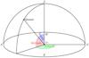 |
Fig. 1. Coordinate system showing the positions of the observer (O) and the source (quasar) on the sky. The zenith angle, altitude, and azimuth are shown in blue red, and green, respectively. |
Figure 2 illustrates the optical fibre and quasar geometries. To facilitate calculations, we positioned the origin of the coordinate system at the fibre centre at λ = λ0, with axes defined as in Fig. 2. We refer to this simply as the fibre centre. The quasar seeing profile has a radius  , where FWHM is the full width at half maximum intensity of the quasar seeing profile. Telescope guidance imperfections, perturbations in temperature, humidity and pressure of the atmosphere, as well as deviations from estimated observation times, will cause the quasar centre to move by Δx along the x-axis. The quasar centre at λ ≠ λopt is offset by Δy along the y-axis due to atmospheric differential refraction (Filippenko 1982). The quasar profile will therefore lie partially outside of the fibre area for large enough values of
 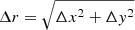 . From this, it follows that a fraction of the incoming quasar light will be lost at certain wavelengths and the flux underestimated (Barnes & Walsh 1988).
 |
Fig. 2. Fibre and seeing profiles in the plane of the detector. The y-axis is aligned with increasing altitude. The black circle represents the fibre with a radius R. The red dot and circle represent the quasar position and profile; i.e. the σ of the quasar Gaussian seeing profile. The red shaded area illustrates the light lost. To calculate the captured flux, we integrate the normalised quasar light intensity within the fibre radius. The figure is adapted from Barnes & Walsh (1988). |
Figure 3 shows eight BOSS exposures of the quasar J022836.08+000939.2. The Margala et al. (2016) correction has not been applied. The spectral shapes are seen to differ for individual observations. Whilst we cannot be sure that quasar variability is not in part responsible for the observed spectral shape differences, the fibre offset problem will also contribute to the apparent spectral shape variations.
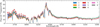 |
Fig. 3. Eight uncorrected SDSS BOSS observations of the quasar J022836.08+000939.2 (Thing ID = 97003678) in DR13, smoothed by a box-car filter of 10 pixels in width. The quasar was observed between September 2011 and October 2013. The spectral shape of the quasar continuum is seen to vary for different observations. If spectral index and/or absolute flux do not change, this variation probably occurs due to a fibre positioning offset, as first noted by Lee et al. (2013) and discussed in this paper in Sect. 2. The numbers in the legend refer to the observations listed in Table 2. |
2.3. Calculating the fibre offset Δy
We now consider a general case in which the fibre is centred at wavelength λ0, and calculate the flux coming from the quasar which is collected by the fibre as a function of wavelength. This requires knowledge of the distance of the two centres (the target and the fibre) along the y-axis, denoted by Δy (see Fig. 2). Δy is determined by the zenith angle, Z; the difference in the refractive indices of air, n, at wavelengths λ and λ0. Δy (measured in arcseconds), is then calculated as follows (Smart 1931; Filippenko 1982):
![Mathematical equation: $$ \begin{aligned} \Delta y (\lambda ,\lambda _0)&= y(\lambda ) - y(\lambda _0)\nonumber \\&\approx 206265\left[n(\lambda ) - n(\lambda _0)\right] \tan Z. \end{aligned} $$](/articles/aa/full_html/2021/11/aa41392-21/aa41392-21-eq4.gif) (2)
(2)
The refractive index, obtained using lunar laser ranging (Marini & Murray 1973), is given by
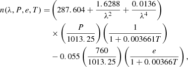 (3)
(3)
where
λ = wavelength in microns,
P = atmospheric pressure in millibars,
e = partial water vapour pressure in millibars, and
T = air temperature in degrees Celsius.
The SDSS FITS header for each quasar exposure provides the atmospheric pressure in inches of mercury. Equation (3) requires P in millibars, given by P(mb) = 33.86389 P(inches of mercury).
The second term (involving e) in Eq. (3) cancels in the subtraction of Eq. (2) so in practice is not needed, but for completeness we illustrate the full calculation of n(λ, P, e, T). The SDSS FITS headers provide the relative humidity, H, for each exposure. The partial water vapour pressure is
 (4)
(4)
where
![Mathematical equation: $$ \begin{aligned} e^\prime (P,T) =&\left[1.0007 + (3.46 \times 10^{-6}P)\right]\nonumber \\&\times 6.1121\exp \left[\dfrac{17.502\;T}{240.97+T}\right]\cdot \end{aligned} $$](/articles/aa/full_html/2021/11/aa41392-21/aa41392-21-eq7.gif) (5)
(5)
(Buck 1981).
We evaluate Δy using Eq. (2) for each spectrum over the observed wavelength range.
2.4. Flux correction calculation
Equation (2) provides the physical offset of the quasar seeing profile from the fibre centre as a function of wavelength. The SDSS pipeline data reduction procedure assumes (incorrectly) that the quasar and calibration stars are both centred at λ0 = 5400 Å. The flux correction function derived here corrects for this assumption, as does the correction function of Margala et al. (2016).
However, here we take into account an additional point that is not included in the SDSS pipeline correction; the fibre offset corrections derived in Margala et al. (2016) assume that the seeing profile (measured empirically for each exposure at 5000 Å) is constant with wavelength. The correction function described in this paper allows for wavelength dependence according to
 (6)
(6)
for example, Roddier (1981), Meyers & Burchat (2015), where σ0 is the seeing measured by the SDSS secondary camera during observations using a filter with maximum throughput at 5000 Å. We note the measurements by Dey & Valdes (2014) (some of which do not detect the trend in Eq. (6)), but we opted to use the latter since this is theoretically sound.
The normalised quasar intensity is, in Cartesian coordinates,
![Mathematical equation: $$ \begin{aligned} \rho (x,y) = \frac{1}{2\pi \sigma ^2}e^{-\left[(x - \Delta x)^2 + (y - \Delta y)^2\right]/2\sigma ^2}, \end{aligned} $$](/articles/aa/full_html/2021/11/aa41392-21/aa41392-21-eq9.gif) (7)
(7)
where x, Δx, y, Δy, are illustrated in Fig. 2.
Transforming to polar coordinates, the normalised quasar intensity becomes
 (8)
(8)
where d is the distance from the quasar centre and is a function of r and θ (illustrated in Fig. 2).
Atmospheric refraction shifts the quasar centre in the y direction only. Any fibre-quasar misalignments perpendicular to the atmospheric refraction direction, Δx, can also in principle create spectral shape changes, since the seeing profile depends on wavelength. However, we assume that Δx is small compared to refraction offsets from Eq. (2). We thus put Δx = 0 and ignore all misalignments not associated with atmospheric refraction.
The law of cosines relates d to the fibre offset Δy and the coordinates of point P, r, and θ:
 (9)
(9)
Allowing for the fibre truncating the Gaussian (asymmetrically when λ ≠ λ0), the fraction of incident quasar light entering the fibre is
 (10)
(10)
where R is the fibre radius. Expressed as a function of λ and λ0, Eq. (10) is
 (11)
(11)
We now define the throughput functions as
 (12)
(12)
and
 (13)
(13)
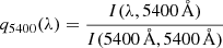
which we calculate for each quasar. I(5400 Å, 5400 Å) and I(4000 Å, 4000 Å) signify the quasar light collected at λ = λ0; that is, when the quasar’s centre coincides with the fibre’s centre, and they serve as normalisation constants.
The correction function, C, is the ratio of the throughput functions,
 (14)
(14)
The corrected quasar flux f(λ) then becomes
 (15)
(15)
where f′(λ) is the uncorrected quasar flux at wavelength λ.
2.5. Sensitivity of the correction function to different variables
Section 2.4 illustrates that the fibre offset correction calculation depends on air pressure, temperature, seeing, and zenith angle. It is therefore of interest to examine the relative importance of these parameters. To this end we calculate Eq. (14) for representative ranges in each parameter, keeping three parameters constant and varying only one at a time. The parameter ranges used for this purpose were obtained empirically from the observed ranges seen in the quasar sample described hereafter.
Figure 4 illustrates the results. From top to bottom, we show air pressure (P, black curves), air temperature (T, red curves), atmospheric seeing (σ, blue curves), and zenith angle (Z, green curves). In each panel, only one parameter is allowed to vary and the non-varying parameters are held fixed. The left hand column illustrates C(λ) for constant seeing, whilst the right hand column shows the results for wavelength-dependent seeing as per Eq. (6). The non-varying parameters are fixed at their average values, taken over the sample of observations used in this work: p = 729.91 mbar, T = 8.58°C, σ = 1.58″, Z = 39.11°. The following values are used for (a) pressure: 726, 728, 730, and 734 mbar; (b) temperature: −5, 0, 5, 10, and 15°C; (c) seeing: 1.0, 1.2, 1.4, 1.6, 1.8, 2.0, 2.2, and 2.4 Å; and (d): zenith angle: 20, 25, 30, 35, 40, 45, and 50°. We note the different y-axis scale for the bottom panel, when zenith is varied. The correction function evidently depends most sensitively on the zenith angle, with seeing being the next most sensitive parameter. Variations in temperature and pressure have the least significant effect.
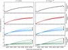 |
Fig. 4. Relative importance of the variables’ air pressure, air temperature, seeing, and zenith angle. In the left column, seeing is independent of wavelength, whilst the right column shows the results for wavelength-dependent seeing. The varying parameter is indicated on the right hand side. The other three parameters in each panel are set at mean values using non-repeated MJD settings in Table 2. The arrows in each panel indicate the direction in which the correction function moves as the parameter value increases. Line thickness also increases with the increase in the parameter value. See Sect. 2.5 for details. |
3. Selecting SDSS quasars with multiple exposures
In order to examine the impact of applying Eq. (14), we use a sample of SDSS DR13 quasars. More specifically, we chose quasars with multiple exposures with good signal-to-noise ratios (S/N). By applying the correction to each exposure and then examining internal consistency for each set for a given quasar, we may be able to quantify any potential spectral shape improvement resulting from our fibre offset correction. The same sample can also be used to check for consistency between the Margala et al. (2016) and our corrections. We also compare results obtained using corresponding DR16 spectra (Ahumada et al. 2020), which have had the Margala correction applied but to individual 15-min exposures (rather than only to summed one-hour spectra).
The quasar selection criteria used for this purpose are contained within the file spAll-v5_9_0.fits1 (a summary file of metadata such as target coordinates, redshifts, photometry, identifiers, classification, number of exposures, etc.). The eight selection criteria applied are: (1) LAMBDA_EFF = 4000 (a modified fibre, centred at λ = 4000 Å, was used); (2) OBJTYPE = ‘QSO’ (the object was targeted as a quasar); (3) CLASS = ‘QSO’ (the object was subsequently classified as a quasar); (4) ZWARNING = 0 (no known issues with redshift estimate); (5) NSPECOBS > 4 (the quasar was observed more than four times); (6) SN_MEDIAN_ALL > 10 (S/N per observation > 10 over the entire wavelength range and for all observations); (7) ANCILLARY_TARGET1 = 0 (not targeted as a part of any quasar variability or broad absorption line programmes); (8) MJD > 55447 (the date after which weather information was routinely saved into FITS file headers).
These stringent criteria result in a sample of nine quasars. For five of these quasars, we could not obtain a good power-law fit to the quasar continuum regions (Sect. 4.2). The spectrum of one resembled a type 1 AGN (‘Thing ID’ 97024300) and one was a strong broad absorption line quasar (110633310). In the remaining three cases (70363665, 78014536, and 106364494), a power law gave a reasonable fit to the uncorrected BOSS spectra; however, after applying the correction functions, a power law no longer produced a good fit, for reasons unknown. This left us with only four quasars, which we discuss now. Basic information regarding the four quasars is given in Table 1, together with their unique identifiers in the SDSS database, ‘Thing ID’ and ‘Obj ID’. We find that the Thing ID for the same quasar differs between DR12 and DR13, so we also included the Obj ID for each quasar. ObjID identifies an object in the SDSS image catalogue used by the Catalog Archive Server2.
Details on the quasars used in this work.
4. Applying fibre offset corrections to 4 quasars with multiple BOSS exposures
Ideally, we would be able to draw upon completely independent (and more precise) observations of the four quasars above, enabling comparisons with BOSS exposures before and after applying fibre offset corrections. Unfortunately, the available data permit this only in a limited sense. We thus proceeded by exploring the following two questions: (1) does applying fibre offset corrections produce greater consistency between the individual quasar exposures, and (2) does it also result in more consistent spectral index estimates? Individual exposures of the four quasars we used are tabulated in Table 2.
Quasar exposures used.
Assuming atmospheric differential refraction is the most significant factor contributing to incorrect spectral shapes, we would expect that applying the flux correction procedure would result in consistent spectral shapes for individual exposures on the same quasar. Figure 5 shows the BOSS observation of J022836.08+000939.2 (plate 3647, MJD 56596, fibre 776, 4 × 15 min exposures, co-added), before and after correcting for the fibre offset problem. The SDSS-I observation is also shown (unaffected by the fibre offset problem, plate 2635, MJD 54114, fibre 621). We can see that the corrected BOSS spectrum is in very good agreement with the SDSS-I spectrum. We comment hereafter on the similarity between the flux correction method described in this paper and that of Margala et al. (2016). On this basis of the result illustrated in Fig. 5, one may infer that the correction works well. However, the interpretation is not straightforward, as the following test shows.
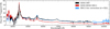 |
Fig. 5. Corrections of a single observation. The BOSS spectrum of J022836.08+000939.2 (Plate: 3647, MJD: 56596, Fibre: 776) before (red) and after (blue) correcting for the fibre offset problem. The SDSS-I observation (Plate: 2635, MJD: 54114, Fibre: 621), unaffected by the fibre offset problem, is shown in black. |
Figure 6 illustrates all eight BOSS observations of J022836.08+000939.2, before and after applying our correction for the fibre offset problem. The correction functions for this set of observations are shown in Fig. 7, which clearly shows that the effect of wavelength dependence is significant. The effect the corrections have on the spectral shapes of the observations is evident from Fig. 7; the corrections lower the fluxes at wavelengths λ ≲ 4538 Å, while increasing the fluxes at wavelengths λ ≳ 4538 Å.
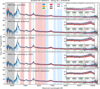 |
Fig. 6. Eight BOSS observations of the quasar J022836.08+000939.2 (Thing ID 97003678). Individual observations are shown as coloured lines, with the legend showing the observation ID in Table 2. The wording within each box shows which correction has been applied (no correction has been applied in the top box, DR13). The inset in each panel illustrates a shorter wavelength region in more detail, giving a clearer view of the scatter between multiple exposures. The shaded areas show the regions used to calculate ξ2 and its associated error, Eqs. (16) and (17), and results listed in Table 3. The different colours correspond to the four wavebands used. The vertical dashed line around 4538 Å shows the point at which spectra are normalised to a common flux. The spike at 5600 Å is due to a cosmic ray hit. |
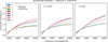 |
Fig. 7. Correction functions (Eq. (14)) for the eight observations of J022836.08+000939.2 shown in Fig. 6. The numbers in the legend correspond to the observation IDs in Table 2. |
4.1. Consistency before and after correction
One way to quantify the correction procedure effectiveness is to compare the consistency between multiple exposures of the same quasar, before and after correcting for the fibre offset problem. To do this, we calculate the variance weighted departures from the mean flux squared3 within wavelength regions:
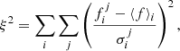 (16)
(16)
where the subscript i corresponds to pixels within one spectrum and the superscript j refers to different spectra of the same quasar. The quantity ⟨f⟩i is the ordinary (unweighted) mean flux in the ith pixel, averaged over all j spectra of the same object. We also tried using a weighted mean for ⟨f⟩i. Whilst the numbers changed somewhat, this did not alter any of our conclusions.
Before calculating Eq. (16), we normalised the observations of individual quasars to a common flux level in order to remove possible different flux levels remaining in the reduced spectra. These could be caused by, for example, time variations in the quasar continuum or sky transparency variations. We did this by calculating the mean flux across all exposures in the region where the correction function crosses unity, in the wavelength range 4538 ± 10 Å, and normalising to a common value. We used this specific range (rather than the entire spectrum) because we expect the spectral fluxes to be correct here.
Furthermore, we excluded wavelength regions contaminated with strong quasar and/or sky emission lines from calculating the spread as per Eq. (16). The quasar emission lines we exclude are the Lyman-α, Si IV and O I], C IV, and C III] lines, falling in the following (quasar rest frame) wavelength ranges: 1160 ≤ λ ≤ 1280 Å, 1360 ≤ λ ≤ 1445 Å, 1500 ≤ λ ≤ 1580 Å, and 1845 ≤ λ ≤ 1955 Å (respectively). We searched for strong sky lines in the sky emission line atlas by Hanuschik (2003), which contains 2810 emission lines identified in high-resolution (R ≈ 45 000) observations made by the Ultraviolet and Visual Echelle Spectrograph (UVES). We identify 169 lines (in the Hanuschik 2003 sample) that have a measured FWHM > 0.15 Å and flux > 5 × 10⁻¹⁶ erg s−1 cm−2 Å−1. In practice, this means that we generally exclude the pixel containing the sky feature plus two pixels either side of each feature; that is, we exclude approximately 2 × FWHM for each feature. Inspecting the data, this seemed to be appropriate. The initial pipeline processing of the data attempts to remove cosmic rays, although some are inevitably likely to remain. We did not make any additional attempt to detect and remove cosmic rays.
To assess how well the correction works, the scatter between independent exposures of the same quasar prior to and after applying the correction can be compared, using the uncertainty on ξ2:
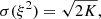 (17)
(17)
where K is the number of degrees of freedom; that is, the number of pixels falling into the wavelength region across all considered spectra. We next discuss the results for each quasar individually.
4.1.1. J022836.08+000939.2, Table 3
The table provides the numerical values from Eqs. (16) and (17) for the quasar J022836.08+000939.2. Measurements are made in four wavelength bands, as shown in the table. Corrections are listed prior to a fibre offset correction and after applying the Margala correction, our correction with constant seeing, our correction with wavelength-dependent seeing, and the DR16 correction. The DR16 correction is the Margala correction, except it is applied to individual 15-min exposures prior to co-adding exposures rather than to summed one-hour spectra. The bottom row in Table 3 gives the values obtained using the all four regions simultaneously; that is, it illustrates the overall benefit (or otherwise) of each correction method.
Comparing agreement between individual exposures for the quasar J022836.08+000939.2 (Thing ID 97176486) for each correction.
Inspecting the values of ξ2 in Table 3, the Margala correction and our comparable correction (σ = const.) provide only a slight improvement for the lowest wavelength region but make dramatic improvements for the three higher wavelength regions. Our second correction (σ = f(λ)) improves the consistency further in all four wavelength regions, as expected given the clear importance of the wavelength dependant seeing correction (Fig. 4). The DR16 method improves consistency in three out of four regions (see discussion in the next paragraph). Overall (bottom row in Table 3), the two σ = const. methods perform almost identically, and the σ = f(λ) and DR16 methods improve further (in that order).
Interestingly, the DR16 correction works better than the wavelength-dependant seeing correction in the four highest wavelength regions, but somewhat worse the lowest wavelength region. The reason for DR16 providing a worse correction for the lowest wavelength region is unknown but may be related to the lack of wavelength-dependent seeing in the DR16 correction and/or an inaccurate absolute seeing value in the spectral FITS header. We did not investigate this further. The generally better performance of the DR16 correction for this quasar (i.e. in four out of five regions) highlights the importance of applying these corrections to individual rather than summed spectra. Presumably, if the DR16 correction included wavelength-dependant seeing, even better agreement between individual exposures would be seen.
4.1.2. J022954.42–005622.5, Table A.1
The Margala correction and our σ = const. correction again perform very similarly, both improving on the uncorrected data consistency. Curiously (and unlike J022836.08+000939.2), our σ = f(λ) correction fails to improve on the two σ = const. corrections (with no obvious explanation). Moreover, the DR16 correction makes little or no improvement in the lowest two wavelength regions, but clearly improves consistency in the two highest wavelength regions. Overall, the DR16 correction again works best.
4.1.3. J023308.31–002605.0, Table B.1
Again, the Margala correction and our σ = const. correction perform very similarly, both significantly improving on the uncorrected case. Our σ = f(λ) correction is marginally worse than the two σ = const. methods for the lowest wavelength region, but it improves consistency for three higher wavelength regions. The ordering of worst-to-best correction is again (Margala + our σ = const. method) our σ = f(λ) and DR16.
4.1.4. J023259.60+004801.7, Table C.1
The results from this quasar are peculiar. All four fibre offset correction methods make the agreement between individual spectra conspicuously worse. The individual spectra are most consistent when no correction at all is applied. This can be clearly seen in Fig. C.1. The effect worsens as wavelength increases. We have no explanation for this. The other three quasars do not show this effect, and, in general, applying the fibre offset corrections improves consistency between individual spectra.
4.1.5. Overall picture
Quasar 4 (J023259.60+004801.7) completely fails to co-operate with the correction methods. If for some reason the data had already been corrected prior to data release, this may explain our findings. However, we have no evidence for that, and the explanation seems unlikely. Lacking any alternative, we therefore assume (with no justification) that this quasar is anomalous, and we proceed to draw general conclusions based on the (more consistent) remaining three cases.
Overall, the Margala and our σ = const. methods perform comparably. Our independent geometric correction thus supports the earlier procedures described in Margala et al. (2016). Adding a wavelength-dependant seeing improves consistency. The DR16 method, which does not include wavelength-dependent seeing but which does apply a correction to individual 15-min exposures rather than to a summed one-hour spectrum, works best. This overall pattern strongly implies (a) that it is indeed important to include wavelength-dependant seeing in the pipeline SDSS procedures (not done at the time of writing this paper) and (b) that the DR16 method is likely to improve significantly when this is done.
4.2. Spectral index measurements using different corrections
Another way in which we can explore consistency between different exposures of the same quasar is to compare spectral indices prior to and after applying a flux calibration correction. One would naturally expect greater consistency after the spectral shapes have been corrected. To compare spectral index measurements, we first select nine small spectral regions that are minimally affected by quasar emission features. The rest-frame regions4 are 1280–1292, 1312–1328, 1345–1365, 1440–1475, 1685–1715, 1730–1742, 1805–1837, 2020–2055, and 2190–2210 Å, illustrated in Fig. 8. We fit a linear function of the form
 (18)
(18)
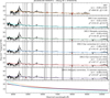 |
Fig. 8. Summed spectrum of the quasar J022836.08+000939.2 (black line). Top panel: DR7 spectrum. The five spectra below the top panel are the same spectral data but corrected in different ways. The continuous coloured line in each panel shows the best-fit power-law continuum to that spectrum, for different flux correction models. The text in each box shows the fitted spectral index and the best-fit χ2 (and its normalised value). The grey shaded areas illustrate the fitting regions. The red dots indicate pixels removed during the power-law fitting procedure. See Sect. 4.2 for details. The six spectral panels all show that a single power law fits well. Lowest panel: six correction functions in slightly more detail. |
where the specific flux fλ has the units erg s−1 cm−2 Å−1, B is a constant, and (by convention) −α is the spectral index. Figure 8 shows that a single power law provides a good fit to the data at rest-frame wavelengths higher than approximately 1280 Å. Figure 4 of Zavarygin & Webb (2019) illustrates this even more convincingly for a composite quasar spectrum. Figure 8 illustrates the summed spectra for J022836.08+000939.2, for different flux calibration corrections. The best-fit power law is shown in each case.
We use two approaches to minimise the impact of absorption features and other corrupted pixels falling within the fitting ranges on the spectral index determination. Firstly, we calculate the mean flux and the mean error in each fitting region and remove all pixels which are ≥3× the mean error away from the mean flux in that region. We then fit the power law of Eq. (18) to the remaining data points, solving for B and α by minimising the quantity
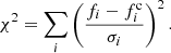 (19)
(19)
Here, the subscript i corresponds to selected pixels within one spectrum, f and σ are the flux and its error (respectively), and fc is the estimated quasar continuum. We iteratively removed pixels for which the absolute values of the normalised residuals are ≥5 until no more pixels are rejected.
The mean spectral indices before and after fibre offset corrections are tabulated in Table 4. Several interesting properties emerge. First, the standard deviation for all eight spectral index measurements is largest for the uncorrected measurements (0.42; see Table 4). All four corrections produce much greater consistency between the eight individually estimated spectral indices. However, a scatter of 0.42 is much larger than the estimated uncertainty on the individual spectral index measurements. This tells us that either 022836.08+000939 undergoes intrinsic time variation or that the SDSS pipeline calibration leaves significant residual uncertainties in the spectral shapes. We are unable to distinguish between these possibilities.
Fitting power law continuum to individual one hour spectra for the quasar J022836.08+000939.
Tables A.2 and B.2 give the results for the second and third quasars and the same general result is seen; applying any of the corrections renders individual spectra more consistent, but the scatter means we cannot favour one correction over another. We avoid the comparison with Table C.2 for the reasons explained above. We learn little more by comparing the results with DR7. Of the three useful quasars, two have previous DR7 observations (unaffected by the fibre offset problem) which we use to measure spectral indices. For J022836.08+000939, −αDR7 = −0.65 ± 0.02, which is inconsistent with any of the four methods shown in Table 4. For J022954.42–005622, −αDR7 = −0.96 ± 0.03. The Margala and DR16 values in the table are consistent, but our two correction methods produce values that are too large. In summary, it turns out that this test is less informative than that described in Sect. 4.1 although it does indicate, in general terms, that the geometric correction methods work.
5. Discussion
We describe a detailed geometric method for applying flux calibration corrections to SDSS quasar spectra, a problem first reported in Lee et al. (2013). An earlier approach by Margala et al. (2016) is also geometric but differs from ours in that we used a correction in which the seeing is wavelength dependent. The results we obtain show that the earlier Margala correction works and that further improvement could be obtained for the default SDSS pipeline if wavelength-dependent seeing is included. We note the two other independent flux correction methods of Harris et al. (2016), Guo & Gu (2016), but since these are based on averaged stellar spectra and not a first-principles geometric approach, we focused our comparisons purely between Margala and the new methods introduced in this paper.
The calculations described here enable an assessment of the relative importance of individual corrections applied to solve the fibre offset problem. The left and right hand columns of Fig. 4 provide a comparison between the four contributions to the overall flux corrections, with and without wavelength-dependent seeing. It is clear that the functions do indeed change significantly, demonstrating the importance of including wavelength-dependent seeing.
We compared four flux corrections: that of Margala et al. (2016), our own two (one with and one without wavelength-dependent seeing), and the DR16 correction (which is the Margala correction but applied individually to original 15-min exposures rather than to grouped, one-hour spectra). By examining the impact of these corrections on quasars with multiple exposures, we were able to see which correction method generated greater consistency between independent exposures. Comparing our own two methods, with and without wavelength-dependent seeing, clearly illustrates the importance of allowing for the latter. Since our method was applied to grouped, one-hour spectra, and the DR16 method was applied to individual 15-min exposures, the results detailed in Sects. 4.1 and 4.2 strongly imply that the current DR16 correction method would improve substantially if wavelength-dependent seeing were to be included.
A final point deserves a mention, although we did not investigate it in this work. Zavarygin & Webb (2019) showed that there are spatially correlated systematic errors in the flux correction function over large scales across the sky. These systematics can emulate cosmological inhomogeneity. The origin of these effects in SDSS data is unknown but should be explored for certain science goals. Such effects should be avoided in any future similar surveys.
We avoid the usual χ2 notation to distinguish between χ2 in Sect. 4.2, where we use it as the goodness-of-fit estimator.
Pâris et al. (2017) also provide spectral indices for two of the four quasars we study here but use very different rest-frame fitting regions. Their regions are seen to contain emission line features in the composite quasar spectrum illustrated in Fig. 4 of Zavarygin & Webb (2019), we thus avoid comparison with their results.
Acknowledgments
JKW thanks the Department of Applied Mathematics and Theoretical Physics and the Institute of Astronomy at Cambridge University for hospitality and support, and Clare Hall for a Visiting Fellowship during part of this work. CCL thanks the Royal Society for a Newton International Fellowship during the early stages of this work. Funding for the Sloan Digital Sky Survey IV has been provided by the Alfred P. Sloan Foundation, the US Department of Energy Office of Science, and the Participating Institutions. SDSS-IV acknowledges support and resources from the Center for High Performance Computing at the University of Utah. The SDSS website is www.sdss.org. SDSS-IV is managed by the Astrophysical Research Consortium for the Participating Institutions of the SDSS Collaboration including the Brazilian Participation Group, the Carnegie Institution for Science, Carnegie Mellon University, Center for Astrophysics | Harvard & Smithsonian, the Chilean Participation Group, the French Participation Group, Instituto de Astrofísica de Canarias, The Johns Hopkins University, Kavli Institute for the Physics and Mathematics of the Universe (IPMU)/University of Tokyo, the Korean Participation Group, Lawrence Berkeley National Laboratory, Leibniz Institut für Astrophysik Potsdam (AIP), Max-Planck-Institut für Astronomie (MPIA Heidelberg), Max-Planck-Institut für Astrophysik (MPA Garching), Max-Planck-Institut für Extraterrestrische Physik (MPE), National Astronomical Observatories of China, New Mexico State University, New York University, University of Notre Dame, Observatário Nacional/MCTI, The Ohio State University, Pennsylvania State University, Shanghai Astronomical Observatory, United Kingdom Participation Group, Universidad Nacional Autónoma de México, University of Arizona, University of Colorado Boulder, University of Oxford, University of Portsmouth, University of Utah, University of Virginia, University of Washington, University of Wisconsin, Vanderbilt University, and Yale University.
References
- Ahn, C. P., Alexandroff, R., & Prieto, C. A. 2012, AJ, 203, 21 [NASA ADS] [Google Scholar]
- Ahumada, R., Prieto, C. A., Almeida, A., et al. 2020, ApJS, 249, 3 [Google Scholar]
- Alam, S., Albareti, F. D., Allende Prieto, C., et al. 2015, ApJS, 219, 12 [Google Scholar]
- Barnes, N. P., & Walsh, P. J. 1988, Appl. Opt., 27, 1230 [NASA ADS] [CrossRef] [Google Scholar]
- Buck, A. L. 1981, J. Appl. Meteorol. (1962–1982), 20, 1527 [CrossRef] [Google Scholar]
- Dawson, K. S., Schlegel, D. J., Ahn, C. P., et al. 2013, AJ, 145, 10 [Google Scholar]
- Dawson, K. S., Kneib, J.-P., Percival, W. J., et al. 2016, AJ, 151, 44 [Google Scholar]
- Dey, A., & Valdes, F. 2014, PASP, 126, 296 [CrossRef] [Google Scholar]
- Eisenstein, D. J., Weinberg, D. H., Agol, E., et al. 2011, AJ, 142, 72 [Google Scholar]
- Filippenko, A. V. 1982, PASP, 94, 715 [Google Scholar]
- Gunn, J. E., Siegmund, W. A., Mannery, E. J., et al. 2006, AJ, 131, 2332 [NASA ADS] [CrossRef] [Google Scholar]
- Guo, H., & Gu, M. 2016, ApJ, 822, 26 [NASA ADS] [CrossRef] [Google Scholar]
- Hanuschik, R. W. 2003, A&A, 407, 1157 [NASA ADS] [CrossRef] [EDP Sciences] [Google Scholar]
- Harris, D. W., Jensen, T. W., Suzuki, N., et al. 2016, AJ, 151, 155 [NASA ADS] [CrossRef] [Google Scholar]
- Kim, T. S., Carswell, R. F., Cristiani, S., D’Odorico, S., & Giallongo, E. 2002, MNRAS, 335, 555 [NASA ADS] [CrossRef] [Google Scholar]
- Lee, K.-G., Bailey, S., Bartsch, L. E., et al. 2013, AJ, 145, 69 [NASA ADS] [CrossRef] [Google Scholar]
- Lehner, N., Savage, B. D., Richter, P., et al. 2007, ApJ, 658, 680 [Google Scholar]
- Lynds, R. 1971, ApJ, 164, L73 [NASA ADS] [CrossRef] [Google Scholar]
- Margala, D., Kirkby, D., Dawson, K., et al. 2016, ApJ, 831, 157 [NASA ADS] [CrossRef] [Google Scholar]
- Marini, J. W., & Murray, C. W. 1973, NASA Technical Report X-591-73-351 [Google Scholar]
- Meyers, J. E., & Burchat, P. R. 2015, ApJ, 807, 182 [NASA ADS] [CrossRef] [Google Scholar]
- Pâris, I., Petitjean, P., Ross, N. P., et al. 2017, A&A, 597, A79 [NASA ADS] [CrossRef] [EDP Sciences] [Google Scholar]
- Penton, S. V., Stocke, J. T., & Shull, J. M. 2004, ApJS, 152, 29 [NASA ADS] [CrossRef] [Google Scholar]
- Rauch, M. 1998, ARA&A, 36, 267 [Google Scholar]
- Roddier, F. 1981, Prog. Opt., 19, 281 [Google Scholar]
- Ross, N. P., Myers, A. D., Sheldon, E. S., et al. 2012, ApJS, 199, 3 [NASA ADS] [CrossRef] [Google Scholar]
- Sargent, W. L. W., Young, P. J., Boksenberg, A., & Tytler, D. 1980, ApJS, 42, 41 [NASA ADS] [CrossRef] [Google Scholar]
- Smart, W. M. 1931, Spherical Astronomy (Cambridge: Cambridge University Press) [Google Scholar]
- Smee, S. A., Gunn, J. E., Uomoto, A., et al. 2013, AJ, 146, 32 [Google Scholar]
- Weymann, R. J., Carswell, R. F., & Smith, M. G. 1981, ARA&A, 19, 41 [NASA ADS] [CrossRef] [Google Scholar]
- York, D. G., Adelman, J., Anderson, J. E., Jr., et al. 2000, AJ, 120, 1579 [NASA ADS] [CrossRef] [Google Scholar]
- Zavarygin, E. O., & Webb, J. K. 2019, MNRAS, 489, 3966 [NASA ADS] [CrossRef] [Google Scholar]
Appendix A: Second quasar details, J022954.42-005622.5 (Thing ID = 74944092)
Same as Table 3, but for the quasar J022954.42-005622.5.
Same as Table 4, but for the quasar J022954.42-005622.5. The SDSS DR7 spectral index is −0.96 ± 0.03.
Appendix B: Third quasar details, J023308.31-002605.0 (Thing ID = 82655414)
Same as Table 3, but for the quasar J023308.31-002605.0.
Same as Table 4, but for the quasar J023308.31-002605.0. This quasar has no DR7 observations so we cannot compare spectral indices.
Appendix C: Fourth quasar details, J023259.60+004801.7 (Thing ID = 110619413)
Same as Table 3, but for the quasar J023259.60+004801.7.
Same as Table 4, but for the quasar J022954.42-005622.5. This quasar has no DR7 observations so we cannot compare spectral indices.
All Tables
Comparing agreement between individual exposures for the quasar J022836.08+000939.2 (Thing ID 97176486) for each correction.
Fitting power law continuum to individual one hour spectra for the quasar J022836.08+000939.
Same as Table 4, but for the quasar J022954.42-005622.5. The SDSS DR7 spectral index is −0.96 ± 0.03.
Same as Table 4, but for the quasar J023308.31-002605.0. This quasar has no DR7 observations so we cannot compare spectral indices.
Same as Table 4, but for the quasar J022954.42-005622.5. This quasar has no DR7 observations so we cannot compare spectral indices.
All Figures
|
Fig. 1. Coordinate system showing the positions of the observer (O) and the source (quasar) on the sky. The zenith angle, altitude, and azimuth are shown in blue red, and green, respectively. |
| In the text | |
|
Fig. 2. Fibre and seeing profiles in the plane of the detector. The y-axis is aligned with increasing altitude. The black circle represents the fibre with a radius R. The red dot and circle represent the quasar position and profile; i.e. the σ of the quasar Gaussian seeing profile. The red shaded area illustrates the light lost. To calculate the captured flux, we integrate the normalised quasar light intensity within the fibre radius. The figure is adapted from Barnes & Walsh (1988). |
| In the text | |
|
Fig. 3. Eight uncorrected SDSS BOSS observations of the quasar J022836.08+000939.2 (Thing ID = 97003678) in DR13, smoothed by a box-car filter of 10 pixels in width. The quasar was observed between September 2011 and October 2013. The spectral shape of the quasar continuum is seen to vary for different observations. If spectral index and/or absolute flux do not change, this variation probably occurs due to a fibre positioning offset, as first noted by Lee et al. (2013) and discussed in this paper in Sect. 2. The numbers in the legend refer to the observations listed in Table 2. |
| In the text | |
|
Fig. 4. Relative importance of the variables’ air pressure, air temperature, seeing, and zenith angle. In the left column, seeing is independent of wavelength, whilst the right column shows the results for wavelength-dependent seeing. The varying parameter is indicated on the right hand side. The other three parameters in each panel are set at mean values using non-repeated MJD settings in Table 2. The arrows in each panel indicate the direction in which the correction function moves as the parameter value increases. Line thickness also increases with the increase in the parameter value. See Sect. 2.5 for details. |
| In the text | |
|
Fig. 5. Corrections of a single observation. The BOSS spectrum of J022836.08+000939.2 (Plate: 3647, MJD: 56596, Fibre: 776) before (red) and after (blue) correcting for the fibre offset problem. The SDSS-I observation (Plate: 2635, MJD: 54114, Fibre: 621), unaffected by the fibre offset problem, is shown in black. |
| In the text | |
|
Fig. 6. Eight BOSS observations of the quasar J022836.08+000939.2 (Thing ID 97003678). Individual observations are shown as coloured lines, with the legend showing the observation ID in Table 2. The wording within each box shows which correction has been applied (no correction has been applied in the top box, DR13). The inset in each panel illustrates a shorter wavelength region in more detail, giving a clearer view of the scatter between multiple exposures. The shaded areas show the regions used to calculate ξ2 and its associated error, Eqs. (16) and (17), and results listed in Table 3. The different colours correspond to the four wavebands used. The vertical dashed line around 4538 Å shows the point at which spectra are normalised to a common flux. The spike at 5600 Å is due to a cosmic ray hit. |
| In the text | |
|
Fig. 7. Correction functions (Eq. (14)) for the eight observations of J022836.08+000939.2 shown in Fig. 6. The numbers in the legend correspond to the observation IDs in Table 2. |
| In the text | |
|
Fig. 8. Summed spectrum of the quasar J022836.08+000939.2 (black line). Top panel: DR7 spectrum. The five spectra below the top panel are the same spectral data but corrected in different ways. The continuous coloured line in each panel shows the best-fit power-law continuum to that spectrum, for different flux correction models. The text in each box shows the fitted spectral index and the best-fit χ2 (and its normalised value). The grey shaded areas illustrate the fitting regions. The red dots indicate pixels removed during the power-law fitting procedure. See Sect. 4.2 for details. The six spectral panels all show that a single power law fits well. Lowest panel: six correction functions in slightly more detail. |
| In the text | |
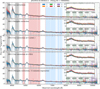 |
Fig. A.1. Same as Figure 6, but for the quasar J022954.42-005622.5. |
| In the text | |
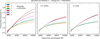 |
Fig. A.2. Same as Figure 7, but for the quasar J022954.42-005622.5. |
| In the text | |
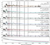 |
Fig. A.3. Same as Figure 8, but for the quasar J022954.42-005622.5. |
| In the text | |
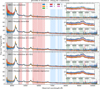 |
Fig. B.1. Same as Figure 6, but for the quasar J023308.31-002605.0. |
| In the text | |
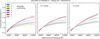 |
Fig. B.2. Same as Figure 7, but for the quasar J023308.31-002605.0. |
| In the text | |
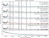 |
Fig. B.3. Same as Figure 8, but for the quasar J023308.31-002605.0. |
| In the text | |
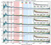 |
Fig. C.1. Same as Figure 6, but for the quasar J023259.60+004801.7. |
| In the text | |
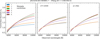 |
Fig. C.2. Same as Figure 7, but for the quasar J023259.60+004801.7. |
| In the text | |
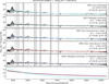 |
Fig. C.3. Same as Figure 8, but for the quasar J023259.60+004801.7. |
| In the text | |
Current usage metrics show cumulative count of Article Views (full-text article views including HTML views, PDF and ePub downloads, according to the available data) and Abstracts Views on Vision4Press platform.
Data correspond to usage on the plateform after 2015. The current usage metrics is available 48-96 hours after online publication and is updated daily on week days.
Initial download of the metrics may take a while.