| Issue |
A&A
Volume 653, September 2021
|
|
|---|---|---|
| Article Number | L11 | |
| Number of page(s) | 14 | |
| Section | Letters to the Editor | |
| DOI | https://doi.org/10.1051/0004-6361/202141783 | |
| Published online | 24 September 2021 | |
Letter to the Editor
A molecular wind blows out of the Kuiper belt
1
LESIA, Observatoire de Paris, Université PSL, CNRS, Sorbonne Université, Univ. Paris Diderot, Sorbonne Paris Cité, 5 place Jules Janssen, 92195 Meudon, France
e-mail: This email address is being protected from spambots. You need JavaScript enabled to view it.
2
Institute of Astronomy, University of Cambridge, Madingley Road, Cambridge CB3 0HA, UK
3
LGL-TPE, UMR 5276, CNRS, Claude Bernard Lyon 1 University, ENS Lyon, Villeurbanne Cedex, France
4
School of Physics, National University of Ireland Galway, University Road, Galway, Ireland
5
Space Science Institute, 4765 Walnut St, Suite B, Boulder, CO 80301, USA
6
LERMA, Observatoire de Paris, Université PSL, CNRS, Sorbonne Université, Univ. Paris Diderot, Sorbonne Paris Cité, 5 place Jules Janssen, 92195 Meudon, France
7
Southwest Research Institute, San Antonio, TX 78238, USA
8
The University of Texas at San Antonio, San Antonio, TX 78249, USA
Received:
13
July
2021
Accepted:
8
September
2021
Abstract
Context. In this Letter we aim to explore whether gas is also expected in the Kuiper belt (KB) in our Solar System.
Aims. To quantify the gas release in our Solar System, we use models for gas release that have been applied to extrasolar planetary systems as well as a physical model that accounts for gas released due to the progressive internal warming of large planetesimals.
Methods. We find that only bodies larger than about 4 km can still contain CO ice after 4.6 Gyr of evolution. This finding may provide a clue as to why Jupiter-family comets, thought to originate in the KB, are deficient in CO compared to Oort cloud comets. We predict that gas is still currently being produced in the KB at a rate of 2 × 10⁻⁸ M⊕ Myr−1 for CO and that this rate was orders of magnitude higher when the Sun was younger. Once released, the gas is quickly pushed out by the solar wind. Therefore, we predict a gas wind in our Solar System starting at the KB location and extending far beyond with regards to the heliosphere, with a current total CO mass of ∼2 × 10⁻¹² M⊕ (i.e., 20 times the CO quantity that was lost by the Hale-Bopp comet during its 1997 passage) and CO density in the belt of 3 × 10⁻⁷ cm−3. We also predict the existence of a slightly more massive atomic gas wind made of carbon and oxygen (neutral and ionized), with a mass of ∼10−11 M⊕.
Results. We predict that gas is currently present in our Solar System beyond the KB and that, although it cannot be detected with current instrumentation, it could be observed in the future with an in situ mission using an instrument similar to Alice on New Horizons but with larger detectors. Our model of gas release due to slow heating may also work for exoplanetary systems and provide the first real physical mechanism for the gas observations. Lastly, our model shows that the amount of gas in the young Solar System should have been orders of magnitude greater and that it may have played an important role in, for example, planetary atmosphere formation.
Key words: Kuiper belt: general / circumstellar matter / planetary systems / solar wind / Sun: heliosphere / interplanetary medium
© Q. Kral et al. 2021
 Open Access article, published by EDP Sciences, under the terms of the Creative Commons Attribution License (http://creativecommons.org/licenses/by/4.0), which permits unrestricted use, distribution, and reproduction in any medium, provided the original work is properly cited.
1. Introduction
The past decade was prolific in terms of detecting gas, mostly CO, C, and O, around main sequence stars, therefore changing the paradigm of evolved planetary systems that were thought to be devoid of gas after 10 Myr. Indeed, most bright exoplanetesimal belts show the presence of gas, as demonstrated recently with ALMA (Moór et al. 2017), and it could be that all these belts have gas at some level, even if undetectable with current instruments. These belts, similar to our Kuiper belt (KB), are made of large bodies colliding with one another and creating dust that can then be observed around extrasolar stars through its emission in the infrared above that of the star, which can be resolved at high resolution (showing e.g., gaps and asymmetries that may be related to the presence of planets).
Recent models show that the best explanation for the CO gas observed co-located with exo-KBs is a secondary production (i.e., the gas is not a remnant of the young planet-forming disks that persist for less than 10 Myr), where CO is released from planetesimals at a rate proportional to their collisional frequency (Kral et al. 2016, 2017). Observations of carbon and oxygen atoms are explained as the daughter species of CO photodissociation within the framework of this model. The most massive gas disks with CO masses close to the amount observed in younger planet-forming disks were first called hybrid disks (e.g., Kóspál et al. 2013) because the gas was thought to be primordial and the dust secondary. We can now also explain the gas in these previously considered hybrid disks as entirely secondary because CO released from planetesimals becomes shielded by the carbon produced when it photo-dissociates (and by CO itself through self-shielding), which can then accumulate to large amounts (Kral et al. 2019; Marino et al. 2020).
In addition, recent observations have shown that comets in our Sol ar System start being active as far as the KB distance. The long-period comet (3 Myr) C/2017 K2 (Pan-STARRS) exhibited activity as far as 9–16 au, and models show that dust production, presumably driven by sublimation of CO, needs to have started at the KB (35 au) to explain the photometric data (Jewitt et al. 2021). Historically, there have also been other comets that show distant CO outgassing, such as C/1995 O1 (Hale-Bopp; Biver et al. 2002) or the short-period Centaur-like comets 29P/Schwassmann-Wachmann 1 and 2060 Chiron (Womack et al. 2017).
Given all this new knowledge in terms of CO outgassing in comets and exocomets, we want to explore what it means for our own Solar System. In this paper we tackle the questions of: what gas production rate we would predict for the current KB; whether sublimation would still be active enough in releasing CO as far as the KB distance that it can be detected; whether the dynamics of the released gas around our G2-type Sun is similar to that previously observed (predominantly though not exclusively) around young main-sequence stars; and if gas is released in the KB, how can we detect it and how does it affect the system as a whole.
2. Results
To answer these questions, we first extrapolated the gas production rate in our KB from the most recent extrasolar models. To do so, we computed the dust mass-loss rate in the KB due to collisions using a state-of-the-art model of dust in our Solar System (Vitense et al. 2012; Morbidelli et al. 2021). According to extrasolar models that fit most observations to date (Kral et al. 2017), the gas production rate is proportional to the mass-loss rate of the belt’s collisional cascade, and we find (see Appendix B) that ∼10−9 M⊕ Myr−1 of CO gas should be released in the current KB. The model’s idea, which fits extrasolar observations, is that large planetesimals are composed of ∼10% CO (see Kral et al. 2017), which is released along with collisions that produce the observed dust (though the detailed physical mechanism is not constrained), either at the top (large, kilometre-sized bodies) or farther down the collisional cascade, but before solid bodies are ground down to dust and expelled by radiation pressure. We also used a more direct approach, relying on the counting rate of the New Horizons dust counter to determine the dust production rate (rather than a numerical model) and arrived at the same value for the gas production rate. We also tested a different, more physically motivated model for releasing the CO and assumed it comes from the slow heating provided by the Sun over long timescales, which warms up large bodies at greater depths as time goes by and releases the CO in these increasingly deeper layers. We find that, after 4.6 Gyr of evolution, only bodies larger than about 4 km can still contain CO (smaller bodies would have lost it already), and all together they release CO at a rate of ∼2 × 10⁻⁸ M⊕ Myr−1. In this model, a single 30 km radius planetesimal would release around 10−14 M⊕ Myr−1 – much lower than what can be detected with missions targeting specific Kuiper belt objects (KBOs; e.g., Lisse et al. 2021). Figure 1 shows the temporal evolution of the release rate, which goes down with time as only larger and larger bodies can participate as time goes by (see Appendix A). We note that this means that sampling the material in the KB now would not lead to the primordial volatile composition of planetesimals. We also tested this slow stellar-driven heating model on more massive belts (similar to those observed around extrasolar systems) and show that it provides the right order of magnitude to explain CO observed around younger exosystems, which may provide the first physical explanation for their ubiquitous CO presence.
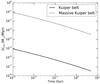 |
Fig. 1. CO gas production rate in the KB ṀCO as a function of time as predicted by our sublimation model (see Appendix A); t = 0 is when the gas release starts, i.e., probably after a few to 10 megayears, and the end of the lines on the right is today. The solid line is for the KB, assuming it starts with a low mass similar to the current KB mass, and the dashed line is for a more massive belt similar to the archetype β Pic belt. |
Comets show a diversity in composition, with a factor of 10–100 variability in the volatile abundance (Bockelée-Morvan & Biver 2017). However, this diversity generally does not appear correlated with the dynamical category. An exception is for CO, whose abundance relative to water appears depleted in Jupiter family comets (JFCs) by a factor of ∼4 on average compared to Oort cloud comets (OCCs; Dello Russo et al. 2016). As we show in Fig. 2, the CO depletion in JFCs compared to other comets is also visible if expressed as a specific CO production rate (i.e., the production rate per unit area QCO/(πD2/4), where D is the equivalent diameter). The top panel of Fig. 2 shows this specific production rate, multiplied by  , as a function of the heliocentric distance (rh) of the measurements. As demonstrated for C/1996 B2 Hyakutake and C/1995 O1 Hale-Bopp (labelled 96B2 and H.B. in the figure), the scaling by
  corrects to the first order for the distance effects and allows a comparison of measurements at different distances. In the bottom panel of Fig. 2, this distance-corrected specific CO production rate is shown as a function of D. In both panels of Fig. 2, JFCs clearly appear CO-depleted with respect to OCCs. As JFCs are thought to originate from the trans-Neptunian region, in particular the scattered disk (SD; e.g. Duncan et al. 2004; Weissman et al. 2020), and since most of them have diameters < 5 km, our calculation that only KB bodies larger than 4 km can retain CO over the age of the Solar System may provide a natural explanation for this behaviour. Interestingly, the observed cumulative size distribution of JFCs may show an excess of comets with radii of 3–6 km (Fernández et al. 2013), similar to the above number; this could account for the diversity of CO abundances within JFCs, although statistics are not sufficient to discern a QCO versus D trend within the JFC group. While Fig. 2 is reassuringly consistent with our sublimation calculations for the KB, we note the following two caveats: (i) the lack of > 5 km JFCs does not allow us to check our prediction that those objects would be less volatile-depleted, and (ii) the low CO production rate of JFCs may also be related to their repeated perihelion passages on their current orbits. We note finally that, with the notable exception of 29P/Schwassmann-Wachmann 1, Centaurs, which are dynamically associated with the SD and JFCs, also appear CO-depleted compared to OCCs (e.g., 10–50 times less CO production per unit surface for Chiron and Echeclus compared to Hale-Bopp; Wierzchos et al. 2017) despite their large, ∼100 km sizes. This is a probable consequence of increased outgassing over their 106 − 107 year lifetime orbits at giant planet heliocentric distances.
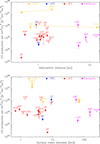 |
Fig. 2. CO production rate per km2 for OCCs (orange), Halley family comets (HFCs, blue), JFCs (red), and Centaurs (purple) of diameter D scaled by the heliocentric distance rh squared – or, in other terms, |

Once CO is released, we find that its dynamics is different from that modelled in extrasolar systems so far (see Appendix E), that is to say, the gas does not evolve viscously inwards as expected in massive disks (Kral et al. 2016). This is due to two reasons. First, the gas quantity we find in the KB is very small and not in the fluid regime, in contrast to systems detected up to now. Second, the majority of gas detections have been around A-type stars (it is mainly an observational bias because more gas is expected in these systems according to models; Matrà et al. 2019), where stellar winds are not important (only stars cooler than about F5 possess significant convective envelopes and thus magnetic fields that can produce strong stellar winds). In contrast, in the Solar System, the solar wind (SW) drives the dynamics of the gas. We find that once released, CO gets pushed outwards by SW protons on timescales of a few years (at a rate between ∼3 to 10 au yr−1, depending on the location; see Appendix F). Some of this CO gets dissociated and ionized, when interacting with SW protons, photons from the Sun, and/or the interstellar medium (see Appendix F), on its way out. However, the ionization and dissociation timescales are of the order of 100 yr, so CO remains the dominant species up to ∼500 au (i.e., well beyond the heliopause, which is the boundary of the heliosphere where the SW is stopped by the interaction with the local interstellar medium (see Appendix D) at ∼150 au (Opher et al. 2020). The daughter products of the CO dissociation, namely C and O, are ionized in ∼100 yr, leading to an ionized atomic component beyond ∼500 au. These ions will then follow the interstellar magnetic lines and get ejected farther into the interstellar medium (see Appendix G). The model predictions for CO, C, and O (neutral and ionized) as a function of distance to the Sun are shown in Fig. 3, and a summary of the model is given in Appendix C.
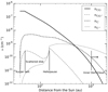 |
Fig. 3. Results of our model for the number density of CO (solid), C and O (dashed), C+ and O+ (dotted), and CO+ (dash-dotted) as a function of distance in our Solar System. The exact shape of the radial profile depends on the heliopause location and geometry, which is not fully modelled in this paper. The assumptions behind this plot are described in Appendix F. We note that the neutral and ionized oxygen number densities are roughly superimposed onto those of carbon. |
Our model leads to a gas wind with a total CO mass (up to 2000 au) of ∼2 × 10⁻¹² M⊕ (i.e., 20 times the CO quantity that was lost by the Hale-Bopp comet during its 1997 passage) and an atomic wind of ∼10−11 M⊕, as summarized in Table 1 (see also Appendix H). The CO density in the belt is predicted to be 3 × 10⁻⁷ cm−3, and the column densities along the midplane are of the order of ∼108 cm−2 for CO, C, and O. We note that our predictions for O may increase by a factor of a few if planetesimals in the KB routinely include O2 ices in quantities similar to those of CO (as may be expected from recent in situ observations of the comet 67 P/Churyumov-Gerasimenko; Bieler et al. 2015) as they are even more volatile than CO.
Results from our gas release model for the total masses, number densities in the belt, and column densities along the line of sight to a star.
In our Solar System, some cometary models predict that planetesimals should still be outgassing in the KB (see Appendix B) at a low rate (Jewitt et al. 2008), and this prediction was recently validated through observations (Jewitt et al. 2021). Upper limits in CO from sub-millimetre studies targeting specific KBOs show that ALMA can detect CO outgassing rates of 2 × 10⁻⁸ M⊕ Myr−1 for a specific comet at KB distances (Jewitt et al. 2008). However, in the case of the KB, the release is more diffuse as the emission comes from many KBOs, and it would be difficult to observe because of the lack of spatial contrast compared to extrasolar systems, where most emission comes from a few beams. We find that Planck and ALMA (in a total power array mode) do not have enough sensitivity to detect the CO rotational lines of the diffuse wind (see Appendix J). The gas accumulated in the midplane of the KB along the line of sight to a background star would create some absorption in the UV on the star spectrum that could be identified as gas in our Solar System. However, we find that only future instruments will potentially be able to detect this faint absorption. The most promising technique would be to use in situ missions similar to New Horizons to detect emission of resonance line scattering of carbon and/or oxygen excited by the Sun’s UV light (see Appendix J). We find that a super-Alice instrument similar to the current Alice UV probe on New Horizons (Stern et al. 2008) but with a larger effective area would reach the low column density level predicted for atoms in the KB. Super-Alice could be built with current technology.
As detailed in Appendix I, we also explored the CO release from Centaurs and find that their current CO mass-loss rate for bodies larger than 4 km is of the same order of magnitude as that predicted by our model for the KB. However, Centaurs being closer to the Sun, CO would be blown out by the SW much faster than in the KB, thus reducing the total CO mass or column that could be observed. We note that the spatial and velocity distributions of this gas are very different from those of gas released in the KB (much closer in and faster), which could allow future observations to distinguish both components.
The presence of current gas predicted by our model in our Solar System would not impact the dynamics of bodies (dust or planetesimals) evolving around the KB. However, we note that in the past, when the KB was much younger and heavier, the release of CO would have been orders of magnitude larger (above the solid line in Fig. 1) and the gas dynamics would have also been much different (e.g., in the fluid regime); this could have potentially led to some interesting effects, such as delivering some CO mass from the KB to planetary atmospheres, as proposed recently for extrasolar systems (Kral et al. 2020). Indeed, in more massive disks, gas becomes optically thick to the SW and does not get pushed outwards. Instead, gas drifts inwards because of viscous evolution and can end up accreted onto planets (see Appendix E). The initial KB may have been much more massive before being affected by potential dynamical instabilities (e.g. Gomes et al. 2005) and could have led to a CO outgassing rate close to the dashed line in Fig. 1, hence providing CO that falls onto the young planets in a greater quantity than from other potential sources, such as impacts (see the comparison between different CO sources in Kral et al. 2020). This is a whole new study that emerges naturally from this work and will be tackled in a different paper.
3. Conclusions
We predict the existence of a gas wind in our Solar System starting at the KB and extending farther out. Our model shows that large, kilometre-sized planetesimals can still lose volatiles after billions of years of evolution due to the slow heating from the Sun, which warms bodies up at greater depths as time goes by. This finding may provide a clue as to why JFCs, thought to originate in the KB, are deficient in CO compared to OCCs. The released CO gas in the KB is constantly produced and then pushed away by the SW, establishing a quasi-steady-state CO disk close to the belt with a calculated current total CO mass of ∼2 × 10⁻¹² M⊕ (i.e., 20 times the CO quantity that was lost by the Hale-Bopp comet during its 1997 passage). We predict a CO density in the belt of 3 × 10⁻⁷ cm−3, as well as the existence of a slightly more massive atomic gas wind made of carbon and oxygen (neutral and ionized) with a mass of ∼10−11 M⊕. This gas cannot be observed with current instrumentation but could be observed with future in situ missions (e.g., a UV instrument similar to Alice/New Horizons but with a larger detector) and may have played an important role in, for example, planetary atmosphere formation in the young Solar System when the gas release rate was much higher (i.e. when the Sun was a few tens of megayears old). Lastly, we show that our new model of gas release due to slow heating of planetesimals by stellar radiation is a promising explanation for the gas detected in exoplanetary systems, which would provide the first real physical mechanism for the origin of the gas.
Acknowledgments
This paper is dedicated to Inaya. We thank the referee for a prompt and helpful review. QK thanks Rosine Lallement and Jean-Loup Bertaux for discussions about the Solar Wind, Heliopause, and Local ISM. QK thanks François Lévrier and Clément Walter for providing information about Planck. QK thanks Andrew Shannon for discussions about latest Kuiper belt collisional models.
References
- Axford, W. I., Dessler, A. J., & Gottlieb, B. 1963, ApJ, 137, 1268 [NASA ADS] [CrossRef] [Google Scholar]
- Balbus, S. A., & Hawley, J. F. 1991, ApJ, 376, 214 [NASA ADS] [CrossRef] [Google Scholar]
- Beust, H., Lagrange-Henri, A. M., Vidal-Madjar, A., & Ferlet, R. 1989, A&A, 223, 304 [NASA ADS] [Google Scholar]
- Bieler, A., Altwegg, K., Balsiger, H., et al. 2015, Nature, 526, 678 [Google Scholar]
- Biver, N., Bockelée-Morvan, D., Crovisier, J., et al. 1999, AJ, 118, 1850 [NASA ADS] [CrossRef] [Google Scholar]
- Biver, N., Bockelée-Morvan, D., Colom, P., et al. 2002, EM&P, 90, 5 [NASA ADS] [Google Scholar]
- Biver, N., Crovisier, J., Bockelée-Morvan, D., et al. 2012, A&A, 539, A68 [NASA ADS] [CrossRef] [EDP Sciences] [Google Scholar]
- Biver, N., Bockelée-Morvan, D., Hofstadter, M., et al. 2019, A&A, 630, A19 [NASA ADS] [CrossRef] [EDP Sciences] [Google Scholar]
- Biver, N., Bockelée-Morvan, D., Lis, D. C., et al. 2021, A&A, 651, A25 [NASA ADS] [CrossRef] [EDP Sciences] [Google Scholar]
- Bockelée-Morvan, D., & Biver, N. 2017, RSPTA, 375, 20160252 [Google Scholar]
- Bockelée-Morvan, D., Lellouch, E., Biver, N., et al. 2001, A&A, 377, 343 [NASA ADS] [CrossRef] [EDP Sciences] [Google Scholar]
- Bockelée-Morvan, D., Biver, N., Colom, P., et al. 2004a, Icarus, 167, 113 [NASA ADS] [CrossRef] [Google Scholar]
- Bockelée-Morvan, D., Crovisier, J., Mumma, M. J., & Weaver, H. A. 2004b, The Composition of Cometary Volatiles, 391 [Google Scholar]
- Brown, G. N., & Ziegler, W. T. 1979, J. Chem. Eng. Data, 24, 319 [Google Scholar]
- Cordiner, M. A., Milam, S. N., Biver, N., et al. 2020, Nat. Astron., 4, 861 [CrossRef] [Google Scholar]
- Crovisier, J., Biver, N., Bockelee-Morvan, D., et al. 1995, Icarus, 115, 213 [NASA ADS] [CrossRef] [Google Scholar]
- Davis, M. W., Gladstone, G. R., Greathouse, T. K., et al. 2011, SPIE, 8146, 814604 [NASA ADS] [Google Scholar]
- Dello Russo, N., Kawakita, H., Vervack, R. J., & Weaver, H. A. 2016, Icarus, 278, 301 [NASA ADS] [CrossRef] [Google Scholar]
- Desch, S. J., & Jackson, A. P. 2021, JGRE, 126, e06807 [NASA ADS] [Google Scholar]
- Dialynas, K., Krimigis, S. M., Mitchell, D. G., Decker, R. B., & Roelof, E. C. 2017, Nat. Astron., 1, 0115 [CrossRef] [Google Scholar]
- DiSanti, M. A., Bonev, B. P., Russo, N. D., et al. 2017, AJ, 154, 246 [NASA ADS] [CrossRef] [Google Scholar]
- Duncan, M., Levison, H., & Dones, L. 2004, Dynamical Evolution of Ecliptic Comets, 193 [Google Scholar]
- Feldman, P. D., Festou, M. C., Tozzi, P., & Weaver, H. A. 1997, ApJ, 475, 829 [NASA ADS] [CrossRef] [Google Scholar]
- Fernández, Y. R., Kelley, M. S., Lamy, P. L., et al. 2013, Icarus, 226, 1138 [NASA ADS] [CrossRef] [Google Scholar]
- Ferrari, C., & Lucas, A. 2016, A&A, 588, A133 [NASA ADS] [CrossRef] [EDP Sciences] [Google Scholar]
- Gladstone, G. R., Stern, S. A., Ennico, K., et al. 2016, Science, 351, aad8866 [NASA ADS] [CrossRef] [Google Scholar]
- Gladstone, G. R., Kammer, J. A., Adams, D. J., et al. 2021, Icarus, 356, 113973 [CrossRef] [Google Scholar]
- Goldsmith, P. F., & Langer, W. D. 1999, ApJ, 517, 209 [Google Scholar]
- Gomes, R., Levison, H. F., Tsiganis, K., & Morbidelli, A. 2005, Nature, 435, 466 [Google Scholar]
- Gomes, R. S., Fernández, J. A., & Gallardo, T. 2008, The Solar System Beyond Neptune, eds. M. A. Barucci, H. Boehnhardt, D. P. Cruikshank, & A. Morbidelli (Tucson: University of Arizona Press), 259 [Google Scholar]
- Greathouse, T. K., Gladstone, G. R., Davis, M. W., et al. 2013, SPIE, 8859, 88590T [NASA ADS] [Google Scholar]
- Groussin, O., Attree, N., Brouet, Y., et al. 2019, Space Sci. Rev., 215, 29 [NASA ADS] [CrossRef] [Google Scholar]
- Gueymard, C. A. 2018, SoEn, 169, 434 [NASA ADS] [Google Scholar]
- Guilbert-Lepoutre, A. 2012, AJ, 144, 97 [Google Scholar]
- Heays, A. N., Bosman, A. D., & van Dishoeck, E. F. 2017, A&A, 602, A105 [NASA ADS] [CrossRef] [EDP Sciences] [Google Scholar]
- Horányi, M., Hoxie, V., James, D., et al. 2008, Space Sci. Rev., 140, 387 [NASA ADS] [CrossRef] [Google Scholar]
- Hosteaux, S., Chané, E., & Poedts, S. 2019, A&A, 632, A89 [NASA ADS] [CrossRef] [EDP Sciences] [Google Scholar]
- Hu, X., Gundlach, B., von Borstel, I., Blum, J., & Shi, X. 2019, A&A, 630, A5 [NASA ADS] [CrossRef] [EDP Sciences] [Google Scholar]
- Huebner, W. F., & Mukherjee, J. 2015, P&SS, 106, 11 [NASA ADS] [CrossRef] [Google Scholar]
- Huebner, W. F., Keady, J. J., & Lyon, S. P. 1992, Ap&SS, 195, 1 [NASA ADS] [CrossRef] [Google Scholar]
- Huebner, W. F., Benkhoff, J., Capria, M. T., et al. 2006, Heat and Gas Diffusion in Comet Nuclei, by ESA Publications Division, Noordwijk, The Netherlands [Google Scholar]
- Izmodenov, V., Malama, Y. G., & Lallement, R. 1997, A&A, 317, 193 [NASA ADS] [Google Scholar]
- Izmodenov, V. V., Lallement, R., & Geiss, J. 1999, A&A, 344, 317 [NASA ADS] [Google Scholar]
- Jewitt, D. C. 2004, From Cradle To Grave: The Rise and Demise of the Comets, 659 [Google Scholar]
- Jewitt, D., Garland, C. A., & Aussel, H. 2008, AJ, 135, 400 [NASA ADS] [CrossRef] [Google Scholar]
- Jewitt, D., Kim, Y., Mutchler, M., Agarwal, J., Li, J., & Weaver, H. 2021, AJ, 161, 188 [NASA ADS] [CrossRef] [Google Scholar]
- Kóspál, Á., Moór, A., Juhász, A., et al. 2013, ApJ, 776, 77 [NASA ADS] [CrossRef] [Google Scholar]
- Kouchi, A., & Yamamoto, T. 1995, Prog. Crystal Growth Charact., 30, 83 [Google Scholar]
- Kral, Q., & Latter, H. 2016, MNRAS, 461, 1614 [NASA ADS] [CrossRef] [Google Scholar]
- Kral, Q., Wyatt, M., Carswell, R. F., et al. 2016, MNRAS, 461, 845 [NASA ADS] [CrossRef] [Google Scholar]
- Kral, Q., Matrà, L., Wyatt, M. C., & Kennedy, G. M. 2017, MNRAS, 469, 521 [NASA ADS] [CrossRef] [Google Scholar]
- Kral, Q., Marino, S., Wyatt, M. C., Kama, M., & Matrà, L. 2019, MNRAS, 489, 3670 [Google Scholar]
- Kral, Q., Davoult, J., & Charnay, B. 2020, Nat. Astron., 4, 769 [CrossRef] [Google Scholar]
- Krijt, S., Schwarz, K. R., Bergin, E. A., & Ciesla, F. J. 2018, ApJ, 864, 78 [NASA ADS] [CrossRef] [Google Scholar]
- Krivov, A. V., & Wyatt, M. C. 2021, MNRAS, 500, 718 [Google Scholar]
- Läuter, M., Kramer, T., Rubin, M., & Altwegg, K. 2020, MNRAS, 498, 3995 [Google Scholar]
- Lellouch, E., Moreno, R., Müller, T., et al. 2017, A&A, 608, A45 [NASA ADS] [CrossRef] [EDP Sciences] [Google Scholar]
- Lisse, C. M., Young, L. A., Cruikshank, D. P., et al. 2021, Icarus, 356, 114072 [CrossRef] [Google Scholar]
- López-Patiño, J., Fuentes, B. E., Yousif, F. B., & Martínez, H. 2017, PhPro, 90, 391 [Google Scholar]
- Luu, J. X., & Jewitt, D. C. 2002, ARA&A, 40, 63 [NASA ADS] [CrossRef] [MathSciNet] [Google Scholar]
- Marino, S., Flock, M., Henning, T., et al. 2020, MNRAS, 492, 4409 [Google Scholar]
- Masuoka, T., & Samson, J. A. R. 1980, JCP, 77, 623 [NASA ADS] [CrossRef] [EDP Sciences] [Google Scholar]
- Matrà, L., Panić, O., Wyatt, M. C., & Dent, W. R. F. 2015, MNRAS, 447, 3936 [NASA ADS] [CrossRef] [Google Scholar]
- Matrà, L., Dent, W. R. F., Wyatt, M. C., et al. 2017, MNRAS, 464, 1415 [NASA ADS] [CrossRef] [Google Scholar]
- Matrà, L., Marino, S., Kennedy, G. M., et al. 2018a, ApJ, 859, 72 [Google Scholar]
- Matrà, L., Wilner, D. J., Öberg, K. I., et al. 2018b, ApJ, 853, 147 [NASA ADS] [CrossRef] [Google Scholar]
- Matrà, L., Öberg, K. I., Wilner, D. J., Olofsson, J., & Bayo, A. 2019, AJ, 157, 117 [NASA ADS] [CrossRef] [Google Scholar]
- McKay, A. J., DiSanti, M. A., Cochran, A. L., et al. 2021, PSJ, 2, 21 [NASA ADS] [CrossRef] [Google Scholar]
- Meier, R. R. 1991, Space Sci. Rev., 58, 1 [NASA ADS] [CrossRef] [Google Scholar]
- Meyer-Vernet, N., & Issautier, K. 1998, J. Geophys. Res., 103, 29705 [NASA ADS] [CrossRef] [Google Scholar]
- Moór, A., Curé, M., Kóspál, Á., et al. 2017, ApJ, 849, 123 [NASA ADS] [CrossRef] [Google Scholar]
- Morbidelli, A., Nesvorny, D., Bottke, W. F., & Marchi, S. 2021, Icarus, 356, 114256 [CrossRef] [Google Scholar]
- Morgado, B. E., Sicardy, B., Braga-Ribas, F., et al. 2021, A&A, 652, A141 [NASA ADS] [CrossRef] [EDP Sciences] [Google Scholar]
- Nahar, S. N. 1999, ApJS, 120, 131 [NASA ADS] [CrossRef] [MathSciNet] [Google Scholar]
- Nahar, S. N., & Pradhan, A. K. 1997, ApJS, 111, 339 [NASA ADS] [CrossRef] [Google Scholar]
- Nesvorný, D., Vokrouhlický, D., Stern, A. S., et al. 2019, AJ, 158, 132 [Google Scholar]
- Ootsubo, T., Kawakita, H., Hamada, S., et al. 2012, ApJ, 752, 15 [NASA ADS] [CrossRef] [Google Scholar]
- Opher, M., Loeb, A., Drake, J., & Toth, G. 2020, Nat. Astron., 4, 675 [NASA ADS] [CrossRef] [Google Scholar]
- Opitom, C., Hutsemékers, D., Jehin, E., et al. 2019, A&A, 624, A64 [NASA ADS] [CrossRef] [EDP Sciences] [Google Scholar]
- Planck Collaboration XIII. 2014, A&A, 571, A13 [NASA ADS] [CrossRef] [EDP Sciences] [Google Scholar]
- Poppe, A. R., Lisse, C. M., Piquette, M., et al. 2019, ApJ, 881, L12 [NASA ADS] [CrossRef] [Google Scholar]
- Prialnik, D., Benkhoff, J., & Podolak, M. 2004, Comets II, eds. M. C. Festou, H. U. Keller, & H. A. Weaver (Tucson: University of Arizona Press), 359 [Google Scholar]
- Rauer, H., Biver, N., Crovisier, J., et al. 1997, P&SS, 45, 799 [NASA ADS] [CrossRef] [Google Scholar]
- Richardson, J. D., Belcher, J. W., Garcia-Galindo, P., & Burlaga, L. F. 2019, Nat. Astron., 3, 1019 [NASA ADS] [CrossRef] [Google Scholar]
- Roth, N. X., Gibb, E. L., Bonev, B. P., et al. 2018, AJ, 156, 251 [NASA ADS] [CrossRef] [Google Scholar]
- Roth, N. X., Gibb, E. L., Bonev, B. P., et al. 2020, AJ, 159, 42 [Google Scholar]
- Rubin, M., Hansen, K. C., Gombosi, T. I., et al. 2009, Icarus, 199, 505 [NASA ADS] [CrossRef] [Google Scholar]
- Rubin, M., Altwegg, K., Balsiger, H., et al. 2015, Science, 348, 232 [NASA ADS] [CrossRef] [Google Scholar]
- Shakura, N. I., & Sunyaev, R. A. 1973, A&A, 500, 33 [NASA ADS] [Google Scholar]
- Stern, S. A., Slater, D. C., Scherrer, J., et al. 2008, Space Sci. Rev., 140, 155 [NASA ADS] [CrossRef] [Google Scholar]
- Tiscareno, M. S., & Malhotra, R. 2003, AJ, 126, 3122 [NASA ADS] [CrossRef] [Google Scholar]
- Vitense, C., Krivov, A. V., Kobayashi, H., & Löhne, T. 2012, A&A, 540, A30 [NASA ADS] [CrossRef] [EDP Sciences] [Google Scholar]
- Wakelam, V., Herbst, E., Loison, J.-C., et al. 2012, ApJS, 199, 21 [NASA ADS] [CrossRef] [Google Scholar]
- Weaver, H. A., Feldman, P. D., A’Hearn, M. F., Dello Russo, N., & Stern, S. A. 2011, ApJ, 734, L5 [NASA ADS] [CrossRef] [Google Scholar]
- Weissman, P., Morbidelli, A., Davidsson, B., & Blum, J. 2020, Space Sci. Rev., 216, 6 [CrossRef] [Google Scholar]
- Wierzchos, K., Womack, M., & Sarid, G. 2017, AJ, 153, 230 [NASA ADS] [CrossRef] [Google Scholar]
- Womack, M., Sarid, G., & Wierzchos, K. 2017, PASP, 129, 031001 [Google Scholar]
- Wyatt, M. C. 2005, A&A, 433, 1007 [NASA ADS] [CrossRef] [EDP Sciences] [Google Scholar]
- Wyatt, M. C., Clarke, C. J., & Booth, M. 2011, CeMDA, 111, 1 [NASA ADS] [CrossRef] [Google Scholar]
- Yamamoto, T. 1985, A&A, 142, 31 [NASA ADS] [Google Scholar]
Appendix A: Sublimation calculations
There are three important timescales for gas release through sublimation. First, the planetesimals need to heat up, via conduction due to the solar influx, to above the CO sublimation temperature of ∼ 25 K (Huebner et al. 2006) on the thermal timescale. Second, the transition from solid to gas (sublimation) must happen on the sublimation timescale; then, the gas must make its way up through the planetesimal pores to finally escape the body on the gas diffusion timescale.
The thermal timescale to heat a layer of thickness Δp is given by τth = (Δp)2/K, where K = κ/(ρcp) is the thermal diffusivity (in m2/s), which we assumed to be of the order of 10−10 for comet-like objects (Prialnik et al. 2004), with ρ the planetesimal bulk density in kg/m3, cp its specific heat in J/kg/K, and κ its thermal conductivity in J/m/s/K. We note that the thermal diffusivity is smaller for cometary material compared to solid amorphous water ice because cometary material is a porous mixture of ices and refractories, including organics. The effects of porosity on the actual effective thermal conductivity (and hence diffusivity) are consequential (e.g. Ferrari & Lucas 2016; Hu et al. 2019). This value is consistent with current measurements of the thermal inertia at the surface of comets (see Groussin et al. 2019, for a review). We calculated that, during the Solar System lifetime (i.e. tS = 4.6 Gyr), the depth to which planetesimals can heat up to the equilibrium temperature of ∼40 K (Krijt et al. 2018) is  km. After 4.6 Gyr, the layers deeper than 4 km should still retain their primordial temperature of 10-20 K (Huebner et al. 2006; Krijt et al. 2018) and planetesimals smaller than about 4 km should have no further gas to release as any primordial CO would have already been lost.
The sublimation timescale, τsub, is given by  , where S = 3(1 − Ψ)/rp is the total interstitial surface area of the pores (of radius rp of order 1 micron; Prialnik et al. 2004) of the material per given bulk volume (with Ψ the porosity taken to be 0.6), PCO = ACOexp(−BCO/T) is the CO saturated vapour pressure (with ACO = 0.12631 in 1010 Pa and BCO = 764.16 in K; Prialnik et al. 2004), and mCO is the mass of a CO molecule. For the temperatures and pressures involved, we find that it takes some 103 yr for a solid CO molecule to turn into its gaseous form.
The gas diffusion timescale is given by τdif = 3/4(Δp)2 (2πmCO/(kbT))0.5/(Ψrp). For the temperatures involved, we find that it takes 104 yr to diffuse upwards from 4 km deep.
The time to heat up the planetesimals significantly is longer by orders of magnitude compared to the time to sublimate or diffuse up. Hence, the thermal timescale will set the gas release rate in planetesimals. We modelled the gas release rate due to thermal heating over time. First, we assumed that the CO mass contained in Nb bodies of size s (taken from a state-of-the-art collisional model of the KB; Morbidelli et al. 2021) within a layer  deep is MCO = 4/3πρfCONb(s3 − (s − Δp)3), where fCO is the CO to solid mass fraction (around fCOinit = 10% in comets).
The derivative of the CO mass that is warmed up by the Sun is  . To compute fCO for different sizes, we calculated, for each size bin and at each timestep (Δt), the potential CO mass MCOinit contained in the Δp layer (assuming nothing was lost) as well as the CO mass that was already lost at time (t), Mlost = ∑tdMCO/dt Δt, and we get fCO = fCOinit(1 − Mlost/MCOinit), yielding in turn dMCO/dt. This model reproduces the expectation that after 4.6 Gyr of thermal evolution only planetesimals bigger than 4 km can participate in the gas release since smaller bodies have lost all their CO by that time. The decrease in the gas release rate with time is mostly due to there being fewer and fewer bodies that can participate in releasing CO. The 10-50 km bodies dominate the gas release in this model. The resulting CO production rate is shown in Fig. 1. A single 30 km radius planetesimal would currently release around 10−14 M⊕/Myr of CO in this model, which is much lower than what can be detected with missions targeting specific KBOs (Lisse et al. 2021).
Scattered disk objects are replenished from various sub-populations of the KB, and possibly the Oort cloud. Their dynamical lifetime is rather long (∼1.8 Gyr, Gomes et al. 2008, though smaller than the age of the Solar System by a factor of 2.5), but the thermal effect on CO sublimation during this period is limited. Objects in the SD spend most of their time at heliocentric distances larger than those in the KB. The time spent close to perihelion is limited, so the layer heated by such passages (10 m at most, computed from the orbital skin depth; see Prialnik et al. 2004) remains much smaller than the 4 km where the CO sublimation front is located (after thermal evolution in the KB). This means that our simple thermal model – which only looks at the deepest layer that can release CO, which in turn only depends on the material as it is a diffusion calculation – will not be affected. We also note that an SD object will spend most of its time in the KB before going to the SD and will finally be ejected, so the SD phase is not dominant overall.
The equilibrium temperature in the Oort cloud as computed through the same energy balance at the surface is extremely low. Other processes may increase it (e.g. cosmic rays, etc., as described for example by Desch & Jackson 2021), but the expected equilibrium temperature is roughly 6-10K (Jewitt 2004), well below the sublimation temperature of CO. Therefore, our model does not predict sublimation of CO for Oort cloud objects.
We note that in our model the CO released in the KB would be coming from pure CO ices and not CO trapped in water, CO2, or other less volatile ices (Kouchi & Yamamoto 1995), the sublimation temperatures of which are too high for them to become gas at KB distances. Therefore, we only expect the most volatile species to be able to be released as gas in the KB. The volatiles with sublimation temperatures lower than 40 K are N2 (22 K), O2 (24 K), CO (25 K), and CH4 (31 K), with the sublimation temperature given in parentheses (Yamamoto 1985). The photo-dissociation timescales can also affect the observability of these species. At the KB, we find photodissociation timescales of 25-62 yr for N2, 8-13 yr for O2, 34-86 yr for CO, and 3-8 yr for CH4 (where the maximum and minimum values correspond to the Sun at its maximum and minimum activity, respectively, and the mean over a solar cycle of 11 yr should be closer to the longer photodissociation timescale; Huebner & Mukherjee 2015). Next, we used the cometary abundances of volatiles as a proxy for the abundance of planetesimals in the KB. Dinitrogen has been observed in a few comets from the ground, for example the comet C/2016 R2 (Pan-STARRS; Opitom et al. 2019), and in situ, for example 67 P (Rubin et al. 2015). At most, the N2-to-CO ratio could be 0.06 (Opitom et al. 2019) in comets formed at large distances, though it is one order of magnitude lower in 67 P. Dinitrogen would thus be even more difficult than CO to observe even though they have similar photodissociation timescales. Dioxygen has also been observed in the coma of 67 P and may be as abundant as CO on the comet (Bieler et al. 2015). Dioxygen photo-dissociates roughly four times faster than CO at the KB, and the daughter neutral oxygen species would accumulate to that created from CO if planetesimals in the KB routinely included O2 ices. As for methane, the CH4-to-CO ratio is roughly 0.1 (Bockelée-Morvan & Biver 2017), and its photodissociation timescale at the KB is roughly 11 times shorter than for CO. Therefore, the released CH4 would also be more difficult to observe than CO.
Data of JFCs, HFCs, OCCs, and Centaurs for which we both have measurements of QCO and diameter. QCO is the CO production rate in s−1, and its error bar is the 1σ uncertainty. D is the equivalent nucleus diameter in km, and rh is the heliocentric distance of the object in au. The upper limits are represented by the 3σ uncertainties.
We also note that collisions would increase the predicted rate because they would expose some fresh CO ices that can be released faster than on a thermal timescale; however, the collisional timescale for bodies larger than 4 km are longer than the age of our Solar System, and this contribution will be negligible for the current KB. Collisions that happened in the early stages of the trans-Neptunian disk could have affected the size distribution of small bodies and released CO on the surface of these bodies, but we note that we used a state-of-the-art size distribution based on observations (Morbidelli et al. 2021) that already accounts for previous evolution. Therefore, the early collisional evolution is implicitly taken into account in our calculations.
Appendix B: Gas production rate calculations
We used two different techniques to estimate the gas production rate in the KB. First, we assumed that the model of gas production that fits detections and non-detections of gas in extrasolar systems (Kral et al. 2017, 2019) is valid for the KB (Model 1). Second, we tested a more physically motivated model that works out the sublimation rates of the bodies in the KB to then derive the total gas production rate in the belt (Model 2).
Model 1 states that the gas production rate is proportional to the mass-loss rate of the planetesimal belt collisional cascade. This is because it is assumed that gas is produced from collisions when solids grind down to dust somewhere along the cascade. The model does not specify the size of the solid bodies that release gas nor the physics behind it. Rather, the model assumes that all CO contained in a large body (∼10% of its mass) is released before it is ground down to dust and ejected because of radiation pressure. The physics of the gas release is not yet known, but it could be due to high-velocity collisions at the bottom of the cascade, to photo-desorption, or to sublimation (which this paper favours), which are all more active for more massive belts that do indeed release more dust. Therefore, the CO gas production rate is roughly equal to the CO fraction of planetesimals times the dust mass-loss rate, the rate at which mass is passed down the cascade from one bin to the other, which is constant throughout the cascade as the new mass injected at the top of the cascade is lost at the bottom at steady state (Wyatt et al. 2011).
We first computed the mass-loss rate from a state-of-the-art model of the KB (Vitense et al. 2012). Using the cross-section density per size decade A (in m2/m3) derived from the simulations of Vitense et al. (2012), we were able to compute the total mass of bodies in a disk of area SKB = 2πRKBΔRKB and scale height H ∼ 0.4RKB (Luu & Jewitt 2002) as Md(s) = A(4/3πs3ρ)SKB(2H)/(πs2) in a given size bin (s). For the KB location (RKB) and its width (ΔRKB), we took 45 and 10 au, respectively (Luu & Jewitt 2002). Then, we derived the dust mass-loss rate as Ṁd(s) = Md(s)/tsurv(s), where tsurv(s) is the lifetime of a solid of size s taken from collisional simulations (Vitense et al. 2012). Assuming a constant CO fraction (fCO) of 0.1 on solid bodies, we then derived the CO gas production rate as ṀCOtot = fCO Ṁd(s), which is constant at all sizes (s) because at steady state the rate of solids that are broken up by collisions between large bodies is equal to the dust mass-loss rate due to radiation pressure. Making the calculation using the small micron-sized dust grains at the bottom of the cascade or for larger bodies at collisional equilibrium, we find ṀCOtot = 10−9 M⊕/Myr.
We also derived the mass-loss rate based on measurements of the student dust counter on the New Horizons mission (Horányi et al. 2008). The number of particles between 0.5 and 5 microns hitting the student dust counter in the KB at 45 au, moving at vNH ∼ 14 km/s, is estimated to be Fd = 1.5 × 10⁻⁴ m−2 s−1 (Poppe et al. 2019). The total mass of grains is then given by Md[0.5−5μm] = (Fd/vNH) m*SKB(2H), where m* is the mean mass of a particle in the 0.5-5 micron size range, given a particle size distribution slope of -2.5 as it is in the Poynting-Robertson (PR) drag (rather than collisional) regime (Wyatt et al. 2011; Vitense et al. 2012). To get the mass-loss rate of grains between 0.5 and 5 microns, we divided by the PR drag timescale as tPR = 400β−1(RKB)2 (in yr, Wyatt 2005), where we took the ratio between the radiation pressure force to that of stellar gravity β = 0.2 based on the mean size of a grain of mass (m*; Vitense et al. 2012). However, to get the mass-loss rate of the cascade, and not just that of the grains captured by the student dust counter, we needed to multiply this by the number of logarithmic bins up to the size at which collisions dominate over PR drag (Wyatt et al. 2011), that is, up to spr = 100 microns (Vitense et al. 2012). We obtained ṀCOtot = 9 × 10⁻¹⁰ M⊕/Myr, namely a gas production rate very close to that found with the previous method.
Model 2 uses the sublimation model described in the previous section. We find that the gas sublimation rate for the KB is dominated by large bodies, > 4 km, after 4.6 Gyr of evolution. Below this size, all CO gas was released because the entire CO inventory had already been sublimed, and the gas production rate drops to zero. To get the final CO production rate, we summed over all the size bins and find 2 × 10⁻⁸ M⊕/Myr, which is roughly a factor of 20 higher than the previous estimates. The temporal evolution is shown in Fig. 1.
We note that comet sublimation models still predict outgassing at large KB-like distances and estimate that a single large Hale-Bopp comet at 40 au would release about 10−10 M⊕/Myr of CO (Jewitt et al. 2008). However, this is valid only if there remains CO ice on the planetesimal surface. As we have shown, CO ice would be long gone from the upper layers after 4.6 Gyr of evolution, and our model predicts a rate about four orders of magnitude smaller for a given large planetesimal similar to Hale-Bopp.
We also checked whether the sublimation model is consistent with the high release rates observed around younger, more massive stars with ALMA. To do so, we took an extreme case: a belt as massive as that of the β Pic system (i.e. more massive than 1000 M⊕ if we assume the belt to be composed of bodies up to 100 km, though bodies may be born smaller; Krivov & Wyatt 2021). To reach a belt of 1000 M⊕, we scaled up the number of bodies in the KB (total mass equal to ∼0.1 M⊕) by a factor of 104 and re-ran our model, leading to the dashed line in Fig. 1. This shows that gas release rates of ∼0.1 M⊕/Myr can be reached with this model when gas is initially released from the young belt.
The gas release rate in the belt of the β Pic system could be up to 0.1 M⊕/Myr (Kral et al. 2016), but we note that the gas release rate necessary to explain the CO mass observed could be lower as there could be sufficient carbon to shield CO from photodissociation in this system (Kral et al. 2019). The temperature conditions of planetesimals in the KB could be similar to that of other exo-KBs since belts tend to form preferentially at a given distance from their star ( ; Matrà et al. 2018a), and so the resulting belt temperature (
 ) is only weakly dependent on the stellar luminosity (56 K for the β Pic extrapolation) and close to that of the KB. We note that the size distribution in young systems could be different to that of the Solar System, which could also increase or decrease the model predictions; however, this is not taken into account here. A more thorough model that includes collisions for young systems and their free parameters, such as the material composition or temperature of the belt, and determining whether such a model could explain all observations, or just those of the less massive belts, for instance, is beyond the scope of this KB-focused paper.
Appendix C: Description of the gas evolution model
We now summarize the model for the evolution of the gas released in the KB so that the reader gets a feel for what mechanisms are at play while reading the more in-depth sections that follow.
The main ingredients used in the gas evolution model for the KB are summarized in Table C.1, and the main timescales in Table C.2. The main ideas go as follows: (i) CO is released from planetesimals in the KB; (ii) CO is quickly pushed outwards with a velocity ≳ 3 au/yr due to collisions with high-velocity (∼ 400 km/s) protons from the SW (and a small fraction of the CO gets ionized and dissociated during these collisions and due to impinging photons from the Sun and the interstellar medium); (iii) most CO gets pushed beyond the heliopause (located at ∼150 au; Dialynas et al. 2017; Richardson et al. 2019) before it has time to dissociate or ionize; (iv) CO finally turns into C+O, and C gets ionized due to photons from the interstellar medium, while O gets ionized due to collisions with protons from the local cloud of the interstellar medium that is colliding with our Solar System; and (v) the ionized atoms then follow the interstellar magnetic field lines and get ejected farther into the local interstellar medium. More details about each step of the model are given in the following sections.
Processes accounted for in this study for the CO evolution once released from the KB. We show the dominant process at the KB location in the column with an asterisk.
Timescales of the dominant processes at play.
Appendix D: Ionization fraction for the gas in the Kuiper belt
We computed the ionization fraction of the main species being studied by equating the ionization rate to the recombination rate. For the Solar System, we took the photoionization probabilities at 1 au (Huebner & Mukherjee 2015) (in s−1) for C, O, and CO: 8 × 10⁻⁷, 4 × 10⁻⁷, and 6 × 10⁻⁷. The recombination timescales are based on the modified Arrhenius equation (in cm3/s) of the form α(T/300 K)βexp(−γ/T). The recombination rate for O+ is given by Nahar (1999): α = 3.24 × 10⁻¹², β = −0.66, and γ = 0. For C+ we used Nahar & Pradhan (1997): α = 2.36 × 10⁻¹², β = −0.29, and γ = −17.6. Finally, for CO+, α = 2.75 × 10⁻⁷, β = −0.55, and γ = 0 are taken from the KIDA database (Wakelam et al. 2012).
One striking difference with previous work on the subject of gas in planetary systems, where models were developed mostly for A stars in young systems, is that in the Solar System oxygen can be ionized because of the presence of numerous UV photons at energies greater than the ionization potential of oxygen (13.6 eV). Solving for the ionization fractions of CO, C, and O analytically, we searched for the electron density (expected to be the main collider here) necessary to get an ionization fraction greater than 0.5 so that we could later estimate (when we get the electron density from the model) whether the different species will be ionized or not. For CO, we find ne < 3 × 10⁻⁴(T/30K)0.58 cm−3. For C, where we also account for the ionization rate of 3.39 × 10⁻¹⁰ s−1 from the interstellar medium, which is greater than the photoionization rate at 45 au (Heays et al. 2017), we find ne < 91(T/30K)0.29 cm−3, and for O we have ne < 13(T/30K)0.66 cm−3.
We also estimated the CO ionization rate through SW electron impact. The density and temperature at the KB of the fast moving electrons (∼ 610 km/s) are 10−3 cm−3 and 3 × 10⁵ K (25.9 eV) (Meyer-Vernet & Issautier 1998). The electron impact ionization rate (for an electron energy of 18 eV) is ke = 5.49 × 10⁻⁹ cm3/s, which we multiplied by 25.9/18 ∼ 1.4 to account for the highest velocities (Rubin et al. 2009). Equating keneSWnCO to the recombination rate of CO+ described above, we find that an electron density lower than 8 × 10⁻⁶ cm−3 is necessary to lead to an ionization fraction of CO greater than 0.5; the contribution of the slow moving electrons is of the same order of magnitude, albeit slightly lower (Meyer-Vernet & Issautier 1998). The photoionization is therefore much more efficient, and electron impacts from the SW can be neglected for CO ionization.
In the SW result section we use the electron density given by our model to provide an estimate of the ionization fraction of the different species. In broad terms (for T close to 20-50 K), C, O, and CO get > 50% ionized at 45 au for ne < 100 cm−3, < 10 cm−3, and < 3 × 10⁻⁴ cm−3, respectively. So, it is most likely that O and C will be close to 100% ionized at 45 au (if they can be produced and remain at 45 au for long enough; see below), and for CO it depends on the details that we investigate in the coming sections and which are complicated by impacts from SW protons pushing CO away faster than it can photo-ionize.
Appendix E: Spreading timescales
In current and past works about gas in planetary systems, the viscous evolution of a gas disk is often parameterized using an α model (Shakura & Sunyaev 1973), which provides a good description in the fluid regime when the Knudsen number (mean free path over gas scale height) is lower than 1. The value of α sets how fast the gas disk spreads as the viscous timescale (tvisc) is given by r2/ν, with the viscosity  , where cs is the sound speed and Ω the orbital frequency. A recent theoretical study shows that the magnetorotational instability (MRI; Balbus & Hawley 1991) may be able to develop in the debris disk regime and produce large α values, of the order of 0.1, owing to the high ionization fraction of the gas in these systems (Kral & Latter 2016). Observations seem to favour high α values as well (Kral et al. 2016; Marino et al. 2020), though this may depend on the emergence of non-ideal MRI effects (such as ambipolar diffusion) as well as the magnetic field strength (Kral & Latter 2016). Taking α between 10−4 and 0.1, we find that the viscous timescale at the KB location can vary from 1.1 Myr to 1.1 Gyr, assuming a gas temperature of 30 K and a mean molecular weight of 28 (gas dominated by CO).
However, the gas density around the KB may be too low to be in the fluid regime, and previous considerations used to describe gas in exoplanetary systems do not apply. When gas density is very low and the Knudsen number becomes greater than 1, then the non-fluid viscosity can be evaluated as follows: ν2 = λmfp cs, with λmfp the mean free path of a gas particle equal to (ngasσcol)−1, where ngas is the gas density and σcol its collisional cross-section. Since the gas scale height is cs/Ω, this regime may happen when ngas < Ω/(σcolcs). We considered the most favourable case of collisions between charged particles (with a greater collisional cross-section) and took  , where Rcc is the cross-sectional radius for a proton calculated by equating kinetic energy to electrostatic energy, so that we get Rcc = e2/(6πϵ0kbTgas), with e the elementary charge and ϵ0 the vacuum permittivity. Thus, we find that the non-fluid regime appears when ngas < ncrit = 3 × 10⁻⁶ cm−3. As for neutral atoms, Coulomb collisions will happen with charged particles. To find the cross-section of, for example, the C+-O collisions, we accounted for the fact that the ion induces a dipole on the neutral atom, which gives birth to an electric repulsion (Beust et al. 1989). The cross-section for neutral-ion interactions is roughly 104 times smaller than for proton-proton collisions, hence increasing ncrit by a factor of 104.
Assuming the CO gas production rate of 2 × 10⁻⁸ M⊕/Myr derived earlier, we find that the ionized carbon produced from CO photodissociation must remain at 45 au for > 25 yr to reach a gas density greater than ncrit and therefore be in the fluid regime. For the case of neutral atoms (e.g. CO, C, or O), they should remain for > 0.25 Myr. In the next section we calculate how long the CO, C, or O can survive at a given position owing to the action of the SW, which we find acts on smaller timescales than viscous spreading in the Solar System. We find that, due to the SW, the gas density cannot increase sufficiently to be in the fluid regime, which is going to drastically change the dynamics of gas compared to previous studies.
Appendix F: Effect of solar wind on gas
We considered the effect of the SW on the KB gas ring. The SW medium density is ∼8 cm−3 at the location of the Earth (1 au), which translates to a density of nSW = 4 × 10⁻³ cm−3 at 45 au (Hosteaux et al. 2019), assuming a 1/r2 drop-off (i.e. constant radial velocity). We first calculated the time between collisions with the SW for each molecule, which is given by 1/(σX − SWnSWvSW), where σX − SW is the cross-section of interaction between X and protons from the SW and vSW is the SW velocity of about 400 km/s. We considered that the cross-section of interaction between ionized SW particles and CO is set by the induced dipole between CO and a proton, as described above in the spreading timescale section. We find that the induced dipole cross-section is σCO − SW ∼ 7 × 10⁻¹⁴ cm2. For CO, we find that there is a collision with a SW proton every 2.7 yr (i.e. before it has time to dissociate or ionize). For an ionized species (e.g. CO+ and proton) with a higher cross-section (see previous section), it is only about 24 minutes. Similar calculations in the local cloud of the interstellar medium, using a velocity of 26 km/s and a proton density of 0.1 cm−3, lead to 1.7 yr and 15 min for neutral and ionized species, respectively (Richardson et al. 2019).
We estimated the rate of collisions with the SW protons in the KB for a given density of atoms or molecules as

where VKB is the KB volume and nX the density of X.
F.1. Basics of the model based on former literature knowledge
We started our calculations as if we were only aware of the models developed for extrasolar systems, mostly for young A stars, as doing so eases the transition to a Solar System model, where the addition of the SW adds another layer to currently used models.
First, we considered the effect of the SW on the CO molecules for which we first assumed a number density (nCO) of 5 × 10⁻⁶ cm−3; this is expected if CO can survive photodissociation for about 50 years, which is close to that value at 45 au in our Solar System. We calculated the mean loss rate of CO due to SW interactions as ṀSW = WSWμmp, assuming that after each collision the high impact velocity gives an outwards kick to the CO molecule. Indeed, working out the momenta for the CO molecule and the high-velocity proton, assuming that it is conserved and that the collision is perfectly inelastic, we find  . Therefore, we were able to solve for the final CO velocity vector, which we find to be 13.8 km/s radially and 4.3 km/s azimuthally. It is indeed already unbound after the first kick. We note that if the collision is perfectly elastic, the final radial velocity could be twice as great. In reality, when the CO and the proton stick together, the collision will indeed lead to a radial velocity of 13.8 km/s (2.9 au/yr), and, otherwise, it will be a value in the range 13.8-27.6 km/s. Given the charge exchange cross-section between SW protons and CO given in Table C.1, we find that exchanges will happen on a ∼100 yr timescale, that is to say, the aftermath of the collision is most likely CO, but the detailed modelling of the collision geometry and properties goes beyond our simple model. We note that there could be multiple collisions before the heliopause is reached at ∼ 150 au. For instance, if the first collision between CO and a proton happens at 45 au after 2.7 yr, then the CO will travel radially for a bit longer than 2.7 yr since the timescale scales as (r/45)2). We calculated, using a mean collision time over the distance travelled, that the next collision will happen at ∼ 55 au, and thus outside the main KB, and that its radial velocity will have doubled. The next collision will happen ∼ 10 yrs later, when the particle is at ∼ 110 au, close to the heliopause. After that, there are no more collisions with protons from the SW as the SW proton density becomes too small given the high velocity of CO: 8.7 au/yr, or 41 km/s. The next collisions will be with the protons from the local interstellar medium, whose density is around 0.1 cm−3 (Izmodenov et al. 1997), finally equalizing the velocities to around 26 km/s after a few years. For ions, the collisions with protons, be they from the SW or the interstellar medium, are very fast, and it takes a few tens of minutes to reach 400 km/s before the heliopause, or 26 km/s beyond it. The transitions are smoother than described above, and the variation of the velocity with distance is represented in Fig. F.1.
Thus, the CO mass-loss rate due to the SW, when it can accumulate for the photodissociation timescale of 50 years due to the Sun radiation, would be ṀSW ∼ 4 × 10⁻⁷ M⊕/Myr, where mp is the proton mass and we take μ = 28. This is higher than the CO gas production rate we found in this study. As such, CO will actually be removed before it has time to photo-dissociate, which will reduce the total CO density we have used so far.
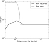 |
Fig. F.1. Sketch of the velocity of particles as a function of distance to the Sun for neutrals (solid) and ions (dashed). The exact shape of the radial profile depends on the heliopause location, which is not fully modelled in this paper and which is assumed to be symmetric, as recently proposed by new studies. The assumptions behind this plot are described in the appendix section on the effect of SW. |
F.2. Improvement and further complexities of the model
To find the number density of CO given its production rate and loss through SW interactions, we equated ṀSW and ṀCOtot and find nCO = 3 × 10⁻⁷ cm−3, which is more than one order of magnitude smaller than the value previously found without properly accounting for the dynamical effect of the SW. This is because there is a collision every 2.7 years at 45 au with high-velocity protons, so CO gets removed roughly 20 times faster than under the action of photodissociation alone. CO will move outwards before being eventually photo-dissociated by UV photons from the interstellar radiation field after roughly 120 yr (i.e. at a distance roughly ten times that of the KB). However, once in the local interstellar medium (i.e. beyond the heliopause at ∼ 150 au; Dialynas et al. 2017), the velocity of CO molecules will be slowed down by collisions with the local interstellar medium protons every few years.
From the CO number density calculation, it is also clear that the CO will be fully ionized by the UV photons from the Sun because we estimate that the electron density is < 3 × 10⁻⁴ cm−3, assuming that electrons come from CO ionization (see CO+ densities in Fig. 3). However, it is not instantaneous, and it will take approximately 100 yr to photo-ionize a given molecule of CO at 45 au (Huebner & Mukherjee 2015). Also, there will be some charge exchanges between CO and protons from the SW that lead to CO+, which may happen faster than photoionization. The cross-section of exchange for protons with an energy of ∼1 keV is ∼1.5 × 10⁻¹⁵ cm2, so exchanges with a CO molecule will happen every 134 yr, at a slightly lower rate than photoionization. We note that photoionization leading to C+ happens 13 times less often and photoionization leading to O+ 15 times less often (Rubin et al. 2009). As for the collisions with protons from the SW, they lead to C+ five times less often and to O+ ten times less often.
As soon as CO becomes CO+, it will leave the system very quickly, as collisions with the SW protons happen every 24 min rather than every 2.7 yr, and the velocity very quickly becomes equal to that of SW protons (i.e. ∼400 km/s). However, CO will start heading outwards after 2.7 yr anyway and may become CO+ on its way out. The final quantity of CO in the KB is indeed therefore set by the frequency of impacts with the SW of 2.7 yr. However, we note that the escape of CO outside of the KB is not instantaneous since the molecule will travel radially at roughly 14 km/s (or ∼2.9 au per yr) after an impact with a SW proton, and it will take a gas particle in the middle of the KB (45 au) roughly 1.7 yr to reach 50 au; as such, CO can slightly accumulate before leaving the belt. Multiplying the CO number density we obtained with ṀSW = ṀCOtot by (1.7+2.7)/2.7, we obtain the mean CO density in the belt (nCO), 5 × 10⁻⁷ cm−3, which will roughly scale as 1/r2 until it dissociates or ionizes. This leads to a surface density at 45 au ΣCO = μmpnCO(2H) ∼ 10−16 kg m−2.
F.3. Modelling the outer regions of the KB
We note that CO will photo-dissociate in ∼120 yr beyond 45 au, while photoionization will operate on a timescale of 107 (r/45 au)2 yr, and proton collisions leading to CO+ in 134 (r/45 au)2 yr. Because CO moves at a rate of 2.9 au/yr after a collision with a proton, it will be at hundreds of au after 100 yr, and the timescales for photoionization and ionization by protons from the SW become > 10, 000 yr. Therefore, CO photo-dissociates before it has time to be ionized. However, the time for CO to move outside of the KB is on average 4.4 yr, and some small fraction of CO will have time to ionize and photo-dissociate. Using an exponential decay law for the time evolution of ionization and photodissociation, we find that 7.3% of CO will be ionized at 45 au and 3.6% will be photo-dissociated. If we assume that most electrons in the KB come from CO ionization, then this gives an electron density (ne) of at least greater than 7.3%×nCO = 2 × 10⁻⁸ cm−3. The CO+ will reach the velocity of the SW protons in a few hours since it collides every 24 minutes with them. Therefore, we expect the CO+ density in the belt to be 7.3%×nCO × (13.8/400) = 2.5 × 10⁻³ nCO = 7 × 10⁻¹⁰ cm−3.
After CO eventually photo-dissociates, an atomic gas component will appear. This leads to Fig. 3, where we show the downwind profile of gas and assume that the heliosphere is not too asymmetric and close to a ball-shape, as recently proposed (Dialynas et al. 2017; Opher et al. 2020), and we do not model the specificities of the heliosheath. To work out the relative gas densities, we also assumed that ions move faster than neutrals, as given by Fig. F.1. The CO produced in the KB would then cross the heliopause (at ∼ 150 au) after roughly 20 yr. Assuming that CO moves at 26 km/s after the heliopause (Opher et al. 2020), CO will be mostly photo-dissociated after 120 yr in total, at ∼ 500 au on the downwind side and slightly farther in on the upwind side because CO gets pushed backwards once it reaches the heliopause. The carbon and oxygen atoms will eventually ionize. The photoionization timescale for C is 94 yr owing to the interstellar medium photons. For O it takes > 13 kyr at > 400 au from the Sun to become ionized since only the Sun’s photons are energetic enough, but O will cross the heliopause and encounter protons from the local interstellar medium and charge exchanges can then happen that will operate in ∼ 110 yr (Izmodenov et al. 1997). Therefore, carbon and oxygen will ionize quickly (we assume 100 yr for both in Fig. 3). The ionized carbon and oxygen will start dominating at ∼500 au on the downwind side. They will then follow the interstellar magnetic field lines (see next section) and get ejected farther into the local interstellar medium.
One of the main conclusions of this model is that CO will move outwards and almost no gas released from the KB will be able to make it inwards towards Neptune. However, we note that it could have been different in the past, when the KB was much more massive and the gas release rate was likely high enough for the gas to be in the fluid regime. In this past situation, the gas became more optically thick to collisions with protons and may have had time to evolve viscously inwards (as described in the viscous evolution section) rather than being pushed outwards, but consideration of this regime is not the purpose of the current paper.
Appendix G: Interaction with the magnetic field
We next analyse the dynamics of an ion produced in the KB, choosing CO+ for the example below. We chose a density n = 10−9 cm−3 of CO+ as a proxy as it is close to the value we find in the previous section. It leads to a mean free path of 2 × 1017 cm for proton-proton collisions (i.e. > 10,000 au), 3 × 1019 cm for charged-neutral collisions, and 3 × 1021 cm for neutral-neutral species collisions (see the SW section for the different cross-sections). We were then able to compare these values with the gyroradius, rg = mvkep/(eB). With the interplanetary magnetic field B ∼ 0.1 nT at the KB (it is 6 nT at Earth and scales as 1/r; Axford et al. 1963), we obtain rg = 8 × 108 cm for a molecule of CO. We could also compare this to the relevant length scale of the problem, L = RKB(cs/vkep), which we find to be equal to L ∼ 2 × 1013 cm.
The gyroradius being smaller than both the mean free path and the relevant length scale, we conclude that ionized species produced in the KB will follow the interplanetary magnetic field lines and escape the Solar System. The same reasoning applies to ionized particles beyond the heliopause in the local interstellar medium, which will then follow the interstellar magnetic lines.
Appendix H: Gas mass, density, and column calculations
Assuming a CO gas production rate of 2 × 10⁻⁸ M⊕/Myr and that CO escapes the KB in 4.4 yr (see the SW section), we get a total CO mass in the KB (40-50 au) of ∼10−13 M⊕, which is roughly the total CO mass that was lost by the Hale-Bopp comet in 1997. This mass translates into the previously calculated mean number density of 3 × 10⁻⁷ cm−3 in the KB. The total CO mass (up to 2000 au) obtained with our model is equal to 2 × 10⁻¹² M⊕, or roughly 20 times the CO mass that was lost by the Hale-Bopp comet during its 1997 passage.
For the carbon and oxygen wind that forms from the CO photo-dissociated molecules, we find that the total atomic masses (up to 2000 au) are ∼6 × 10⁻¹² M⊕ and ∼8 × 10⁻¹² M⊕ for neutral and ionized species, respectively. For the column densities of species X (NX), we integrated along the midplane outwards so that  , with Rin = 45 au and Rout = 2000 au. Table 1 summarizes all these calculations.
Appendix I: Comparison to other sources of CO in the Solar System
Comets release abundant CO when they approach the Sun (e.g. Bockelée-Morvan et al. 2004b). For instance, the 60 km diameter Hale-Bopp comet released a CO mass of ∼10−13 M⊕ during its 1997 passage near the Sun (mostly at its perihelion). This means that 20 such comets could together produce a CO mass comparable to what we predicted for the KB. However, the CO comet production is local, anisotropic, and concentrated near the Sun. Furthermore, after each comet passage CO is quickly blown out by the strong SW and escapes at a speed of several au per month. So, this CO source cannot, in the long run, accumulate and compete with the CO production from the KB.
Centaurs are transient bodies with a dynamical lifetime of ∼106 − 107 yr located between Jupiter and Neptune (Tiscareno & Malhotra 2003). They are expected to originate in the KB (Tiscareno & Malhotra 2003). Despite their large sizes, ∼100 km, the observable Centaurs appear CO-depleted compared to OCCs by a factor of 10 to 50 (Wierzchos et al. 2017). However, there are more than 105 Centaurs larger than about 4 km (Nesvorný et al. 2019) that may still release CO and contribute to a global and diffuse CO gas disk, mainly between 5-30 au, in addition to the CO released in the KB. An order of magnitude of the CO gas quantity that could be released by Centaurs in steady state can be obtained as follows. Using the size distribution given by Nesvorný et al. (2019), and integrating over all bodies between 4 and 50 km diameter (the OSSOS observation range and in agreement with our model that assumes only bodies larger than 4 km may still have CO at the sub-surface), we find that Centaurs have a total surface area of 3.4 × 10⁷ km2, which is 3 × 10³ larger than the area of comet Hale-Bopp.
Assuming that the release rate of Centaurs per unit area is roughly ten times lower than Hale-Bopp (and it can be up to 50 times lower; Wierzchos et al. 2017), using the CO release rate of Hale-Bopp at 10 au (the mean distance of Centaur perihelia is close to 13 au but closer in for active centaurs) of 1028 mole s−1, or 2 × 10⁻⁹ M⊕/Myr (Biver et al. 2002), and assuming that roughly 10% of Centaurs are active (Guilbert-Lepoutre 2012), we find a mean CO outgassing rate of 6 × 10⁻⁸ M⊕/Myr for Centaurs, or ∼ 10−8 M⊕/Myr if the release rate of Centaurs is assumed to be 50 times lower than that of Hale-Bopp at the same distance, rather than 10 times. This order of magnitude shows that Centaurs could potentially contribute to the CO mass-loss rate as much as planetesimals do in the KB, as derived in this paper.
However, the CO gas released by Centaurs is also blown out by the SW much faster than in the KB (e.g. more than 20 times faster because of the increased proton density at ∼10 au), hence decreasing the total mass or column density of CO as compared to that in the KB. A complete modelling of the CO gas released by Centaurs and its evolution is complex and beyond the scope of this paper. However, we note that the two sources of CO gas could be differentiated from their different spatial distributions by measuring the column at different distances from the Sun, for example when an in situ mission similar to New Horizons but with increased sensitivity moves outwards to the KB (see the next section).
Appendix J: Detecting the gas belt
Conceivably, there are different ways of detecting this gas around the KB. The following may not be exhaustive, but the obvious possibilities would be: (i) detection of CO emission at millimetre wavelengths; (ii) detection in the UV (e.g. a resonant carbon line) in absorption against a background star located in the ecliptic; and (iii) in situ detections with future missions similar to New Horizons.
First, we needed to evaluate the population levels for the different lines. Due to the low quantity of electrons we find, the collider density is probably not enough to reach local thermal equilibrium (LTE) and the population levels would be set by the radiation impinging onto the different species. We used a non-LTE code developed for gas in debris disks, including fluorescent excitation (Matrà et al. 2015, 2018b). For the radiation field, we included the cosmic microwave background and the light from the Sun using a state-of-the-art solar spectrum (Gueymard 2018). As can be seen in Fig. J.1, we explored the population levels for a range of excitations and temperatures given the current uncertainties on these. For electron densities below ∼ 10 cm−3, which are the most likely given our model, the population levels are in the radiation regime and converge to a given value. What is clear from this plot is that, regardless of the gas temperature, roughly half of the CO molecules are in the first level and 40% are in the ground state. We use these values to make flux predictions for different lines below.
In the next sections we go over the different possibilities.
J.1. Detectability of CO rotational lines in the millimetre range
The Planck mission was used to make Galactic maps of CO using its great sensitivity (Planck Collaboration XIII 2014). We checked whether any CO gas in the KB could affect these detections and/or whether CO could be seen on Planck maps looking towards the ecliptic. The Planck sensitivity in band 3 (CO J = 1-0 transition at 115 GHz) is roughly 1 K km/s (Planck Collaboration XIII 2014).
Using the population levels we derived, we computed the column density of CO that is needed to get a 3σ detection with Planck (with Eq. 9 of Goldsmith & Langer 1999). We find that 2 × 1015 cm−2 of CO is needed to get a detection, which is orders of magnitude higher than the CO column predictions (∼108 cm−2) from our model. The ALMA non-interferometric total power array mode is more sensitive than Planck given its larger collecting area with 4 × 12 m antennas. Pushing it to its limit, we find that observing the KB for 1000 hours (as of now, 3000 hr per year are devoted to this mode), we would go down to a sensitivity of 0.45 mK km/s. This would lead to a detection for a CO column density of 1012 cm−2, which is still much higher than our CO column predictions. However, using the auto-correlation mode of ALMA with 50 antennas (Cordiner et al. 2020), the sensitivity could be 50/4 = 12.5 times smaller and the detection threshold would then be ∼1011 cm−2. Future arrays that connect more numerous and larger antennas in their non-interferometric mode or using auto-correlation (total power) spectra of interferometric data, as recently done for observing comet tails with ALMA (Cordiner et al. 2020), would allow us to go much deeper. However, we note that we would need to be able to go on and off on the target, which may be difficult given the extent of the KB.
J.2. Detectability of carbon atoms in the UV in absorption against a background star
We now quantify the absorption signal that would be obtained observing a bright background star that happens to lie nearby in the ecliptic plane (i.e. the line of sight would go through the KB). Here we take a bright Sirius-like star at a few parsecs as an example. To estimate the detectability of gas in the KB, we targeted a strong C I resonant line at 1656.9284 angstroms as other lines will be of similar or lower strength. We took the Einstein coefficients from the NIST database and computed the optical depth of the line using Eq. 3 of Matrà et al. (2017). We assumed a full width at half maximum of the line of about 10 km/s, and, using the same non-LTE code as described for CO, we find that the ground state level for carbon is populated at the 99.9% level. We then find an optical depth (τν) of the order of 10−5 for this line.
For an optically thin gas, the flux density of the line is Iν = Iν, bkgexp(−τν), where Iν, bkg is the background star flux density. The signal-to-noise ratio (S/N) of the star is Iν, bkg/σ, where σ is the noise level. For a line detection, we need Iν, bkg − Iν > 3σ at the line centre, which implies a S/N > 3/τν = 3 × 10⁵.
To check whether HST/STIS could detect such a faint signal, we used their Exposure Time Calculator. For a Sirius-like star, we find that the star is too bright to be observed directly with STIS. After using a neutral-density filter, we find that we can reach a S/N of order 100 (for a 2 hour exposure). However, to get a detection here, we would need a S/N of the order of 105, which is too much for HST and could only be tackled by future instruments.
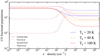 |
Fig. J.1. Population rotational J levels of CO for a range of temperatures and electron densities. The left side shows the radiation-dominated regime, which is the most likely regime for the KB, and the right side has enough colliders to reach LTE. |
J.3. Detectability of gas with an in situ mission
Our Solar System has the advantage over exoplanetary systems in that we can send probes to study its complexity. One such probe is the recent New Horizons mission, which was dedicated to studying Pluto and its satellites, as well as a KBO named Arrokoth.
To detect CO with these in situ missions, the way to go is to look for absorption of species against the Sun or to look for emission of resonance lines (Gladstone et al. 2016). For absorption of CO, its ground state has a complex absorption cross-section at wavelengths < 1000 angstroms (Masuoka & Samson 1980) at around 10−17 cm2. With an equivalent of the Alice instrument that is on board New Horizons (a UV imaging spectrometer), a drop in brightness of ∼ 1% could be detected for a long exposure (Gladstone et al. 2021). Therefore, CO column densities between the instrument and the Sun of the order of 1015 cm−2 could be detected with this technique. This is clearly not enough to detect the CO level predicted by our model.
For some species (mostly atoms), resonance cross-sections can be several orders of magnitude larger than for absorption, which can allow detections of much lower levels of gas in the KB. We now quantify the emission from resonance line scattering for the OI triplet at 1304 angstrom. To get an order of magnitude of the oxygen upper limit, we considered that there is no background emission and that a detection with a S/N of 3 would require about C = 10 counts in the wavelength bin of the emission. For a brightness I = gN (in photons/cm2/s/(4π sr), with g the number of photons scattered per unit time and per atom and N the column density of neutral oxygen), the number of counts in a time t is equal to (Meier 1991)

where Ω is the smallest of the solid angles of the target or detector pixel and Aeff is the effective area of the instrument (the aperture area times all the yields and reflectivities) at a given wavelength (Stern et al. 2008). The pixel size of, for example, the Alice instrument on board New Horizons is much smaller than the KB gas disk solid angle, so we used the Alice pixel size of 0.1 × 0.3 degrees2 to get Ω = 9.1 × 10⁻⁶ sr. At the wavelength of the OI 1304 triplet, the effective area is Aeff = 0.17 cm2 (Stern et al. 2008). The g factor (see Table IV of Meier 1991) was rescaled at 45 au to get g = 9.4 × 10⁻¹⁰ s−1. Integrating the number of counts for 1000 h, we get the upper limit N = 2.4 × 1010 cm−2. It is indeed much more promising than for absorption, but, given our column density predictions for neutral oxygen (2 × 107 cm−2), this is not feasible for now with, for example, Alice. Only future in situ instruments with larger effective apertures and larger pixel sizes will be able to reduce this time: A super-Alice is needed.
For instance, if we use a 7 deg × 0.3 deg micro-channel plate (MCP) for the detector instead of the current 7 deg × 0.1 deg, we gain a factor of three, with a resolution that is still sufficient to distinguish lines of interest (e.g. OI at 130.4 nm). Summing over all pixels instead of just on the 0.1 × 0.3 degree2 pixel mentioned above, which is possible because the emission region is larger than the MCP size, the gain factor becomes 70 as Ω becomes 6.4 × 10⁻⁴. The effective area (Aeff) can also be improved by a factor of ∼3 using MgF2-coated optics, as on the Juno mission, which possess an Alice-like spectrograph (Davis et al. 2011; Greathouse et al. 2013). All together, and without increasing the aperture size, we gain a factor of 200. Using a larger primary would also allow photons to be collected faster and allow sensitivity to be reduced. For instance, going to a six-times-larger primary (24x24cm) would gain another factor of 36 (current airglow aperture is 4 × 4 cm2; Stern et al. 2008) for a total gain factor of ∼7000, which is enough, with some slack to account for model uncertainties, to detect the oxygen predicted by our model in the KB with a reasonable exposure time. This type of super-Alice instrument could be planned with current technology and may fly in the future. We also note that if planetesimals in the KB also contain O2 in a similar quantity to CO, as may be the case in the comet 67 P, our overall prediction for the OI line would also increase by a factor of a few.
All Tables
Results from our gas release model for the total masses, number densities in the belt, and column densities along the line of sight to a star.
Data of JFCs, HFCs, OCCs, and Centaurs for which we both have measurements of QCO and diameter. QCO is the CO production rate in s−1, and its error bar is the 1σ uncertainty. D is the equivalent nucleus diameter in km, and rh is the heliocentric distance of the object in au. The upper limits are represented by the 3σ uncertainties.
Processes accounted for in this study for the CO evolution once released from the KB. We show the dominant process at the KB location in the column with an asterisk.
All Figures
|
Fig. 1. CO gas production rate in the KB ṀCO as a function of time as predicted by our sublimation model (see Appendix A); t = 0 is when the gas release starts, i.e., probably after a few to 10 megayears, and the end of the lines on the right is today. The solid line is for the KB, assuming it starts with a low mass similar to the current KB mass, and the dashed line is for a more massive belt similar to the archetype β Pic belt. |
| In the text | |
|
Fig. 2. CO production rate per km2 for OCCs (orange), Halley family comets (HFCs, blue), JFCs (red), and Centaurs (purple) of diameter D scaled by the heliocentric distance rh squared – or, in other terms, |
| In the text | |
|
Fig. 3. Results of our model for the number density of CO (solid), C and O (dashed), C+ and O+ (dotted), and CO+ (dash-dotted) as a function of distance in our Solar System. The exact shape of the radial profile depends on the heliopause location and geometry, which is not fully modelled in this paper. The assumptions behind this plot are described in Appendix F. We note that the neutral and ionized oxygen number densities are roughly superimposed onto those of carbon. |
| In the text | |
|
Fig. F.1. Sketch of the velocity of particles as a function of distance to the Sun for neutrals (solid) and ions (dashed). The exact shape of the radial profile depends on the heliopause location, which is not fully modelled in this paper and which is assumed to be symmetric, as recently proposed by new studies. The assumptions behind this plot are described in the appendix section on the effect of SW. |
| In the text | |
|
Fig. J.1. Population rotational J levels of CO for a range of temperatures and electron densities. The left side shows the radiation-dominated regime, which is the most likely regime for the KB, and the right side has enough colliders to reach LTE. |
| In the text | |
Current usage metrics show cumulative count of Article Views (full-text article views including HTML views, PDF and ePub downloads, according to the available data) and Abstracts Views on Vision4Press platform.
Data correspond to usage on the plateform after 2015. The current usage metrics is available 48-96 hours after online publication and is updated daily on week days.
Initial download of the metrics may take a while.