| Issue |
A&A
Volume 669, January 2023
|
|
|---|---|---|
| Article Number | A116 | |
| Number of page(s) | 17 | |
| Section | Interstellar and circumstellar matter | |
| DOI | https://doi.org/10.1051/0004-6361/202243729 | |
| Published online | 20 January 2023 | |
Potential effects of stellar winds on gas dynamics in debris disks leading to observable belt winds
1
LESIA, Observatoire de Paris, Université PSL, CNRS, Sorbonne Université, Univ. Paris Diderot,
Sorbonne Paris Cité, 5 place Jules
Janssen,
92195 Meudon, France
e-mail: This email address is being protected from spambots. You need JavaScript enabled to view it.
2
Institute of Astronomy, University of Cambridge,
Madingley Road,
Cambridge
CB3 0HA, UK
3
School of Physics, Trinity College Dublin, The University of Dublin,
College Green,
Dublin 2, Ireland
Received:
7
April
2022
Accepted:
8
November
2022
Abstract
Context. Gas has been successfully detected in many extrasolar systems around mature stars aged between 10 Myr and ∼1 Gyr that include planetesimal belts. Gas in these mature disks is thought to be released from planetesimals and has been modeled using a viscous disk approach where the gas expands inwards and outwards from the belt where it is produced. Therefore, the gas has so far been assumed to make up the circumstellar disk orbiting the star; however, at low densities, this may not be an adequate assumption, as the gas could be blown out by the stellar wind instead.
Aims. In this paper, we aim to explore the timeframe in which a gas disk transitions to such a gas wind and whether this information can be used to determine the stellar wind properties around main sequence stars, which are otherwise difficult to obtain.
Methods. We developed an analytical model for A to M stars that can follow the evolution of gas outflows and target the moment of transition between a disk or a wind in order to make a comparison with current observations. The crucial criterion here is the gas density for which gas particles are no longer protected from the impact of stellar wind protons at high velocities and on radial trajectories.
Results. We find that: (1) belts with a radial width, ΔR, with gas densities <7 (ΔR/50 au)−1 cm−3, would create a wind rather than a disk, which would explain the recent outflowing gas detection in NO Lup; (2) the properties of this belt wind can be used to measure stellar wind properties such as their densities and velocities; (3) very early-type stars can also form gas winds due to the star’s radiation pressure, instead of a stellar wind; (4) debris disks with low fractional luminosities, f, are more likely to create gas winds, which could be observed with current facilities.
Conclusions. Systems containing low gas masses, such as Fomalhaut or TWA 7, or more generally, debris disks with fractional luminosities of f ≲ 10−5(L⋆/L⊙)−0.37 or stellar luminosity ≳20 L⊙ (A0V or earlier) are more likely to create gas outflows (or belt winds) than gas disks. Gas that is observed to be outflowing at high velocity in the young system NO Lup could be an example of such belt winds. Future observing predictions in this wind region should account for the stellar wind in the attempt to detect the gas. The detection of these gas winds is possible with ALMA (CO and CO+ could serve as good wind tracers). This would allow us to constrain the stellar wind properties of main-sequence stars, as these properties are otherwise difficult to measure, since, for example, there are no successful measures around A stars at present.
Key words: circumstellar matter / infrared: planetary systems / solar wind / stars: winds / outflows / stars: mass-loss / Kuiper belt: general
© The Authors 2023
 Open Access article, published by EDP Sciences, under the terms of the Creative Commons Attribution License (https://creativecommons.org/licenses/by/4.0), which permits unrestricted use, distribution, and reproduction in any medium, provided the original work is properly cited.
This article is published in open access under the Subscribe-to-Open model. This email address is being protected from spambots. You need JavaScript enabled to view it. to support open access publication.
1 Introduction
Gas has now been detected in most dense planetesimal belts (observed as bright debris disks) around young, early-type stars >10 Myr (Moór et al. 2017). Gas has also been detected in the vicinity of stars up to a Gyr in age (Matrà et al. 2017b; Marino et al. 2017) and around later-type stars, all the way from M up to A stars (e.g., Marino et al. 2016; Matrà et al. 2019; Kral et al. 2020b; Rebollido et al. 2022), with a remarkable diversity of CO gas masses ranging from 0.1 (e.g., Kóspál et al. 2013; Moór et al. 2017, 2019) to 10−7 M⊕ (Matrà et al. 2017b). The observed CO gas and its daughter products (C and O) are best described as being secondary (Kral et al. 2017, 2019), that is, the gas is released from planetesimals. It is only for the few most massive systems that a primordial origin (i.e., the hypothesis that the gas would be a remnant of the protoplanetary disk phase) has not completely been ruled out. However, there are strong indications that even for these massive systems, the observed gas is of secondary origin (Hughes et al. 2017; Smirnov-Pinchukov et al. 2021) and CO remains abundant thanks to shielding by carbon that is naturally produced in a secondary fashion, as explained in detail in Kral et al. (2019).
These discoveries have prompted several numerical investigations aimed at understanding the origin and evolution of this long-lived gas component. Up to now, this gas has been modeled as a circumstellar disk orbiting the star and mostly co-located with the planetesimal belts. In these models, the gas production rate has been assumed to be proportional to the dust mass-loss rate of the planetesimal belt. This modeling approach was applied to ~200 systems and it can explain most observations to date (Kral et al. 2017). Two exceptions to the standard scenario are given by the detection of an atomic gas wind in η Tel in UV (Youngblood et al. 2021) and probably in optical (Rebol-lido et al. 2018) and also around σ Her in UV (Chen & Jura 2003). The central stars being very early (~A0V), ionised carbon may also become unbound as shown in Kral et al. (2017, Fig. 11) and cannot retain other atomic species through braking Coulomb collisions, as is usually assumed (Fernández et al. 2006).
In addition, when recently studying the low-gas environment of the Solar System Kuiper Belt (KB), Kral et al. (2021) found that the possible secondary gas released (because of progressive internal warming of large planetesimals) by KBOs (Kuiper belt objects) could be directly blown out by the Solar wind without forming a disk-like structure. Indeed, the likely low-gas density in the KB would mean that gas particles are not protected from the Solar wind and each wind proton hitting a gas particle will lead to an ejection (at higher than the local escape velocity) of the gas particle, thus creating a gas belt wind. This KBO gas would have a lower density than expected based on current viscous gas models and a high velocity heading outwards that is characteristic of a wind. Here, the mechanism driving the wind would be stellar wind (SW) and not stellar radiation, as presented in above in the context of η Tel. Stellar winds only have the capacity to affect low-gas density systems, while radiative winds can impact any optically thin gas given that the star is roughly earlier than AOV, which does not apply to many debris disks. The cartoon presented in Fig. 1 shows the classical picture of a gas disk in Keplerian rotation, along with the stellar wind and radiative wind mechanisms that become important at low gas densities and high stellar luminosities, respectively.
In this paper, we aim to trace the behaviour of low density gas in presence of SWs and generalize the current models to any circumstellar gaseous system. Our main goal is to explore the crucial criteria that will determine whether the behaviour of a given gas system will be disk-like or wind-like and whether those “belt” winds can be detected by current instruments. To do so, we developed an analytical model to describe the gas density and velocity in low gas-mass systems where the effect of SWs can become important. We will also investigate whether these belt winds can be used as proxies to determine the SW properties around main-sequence stars that are otherwise hard to measure (Johnstone et al. 2015a), especially for A stars where no measurements have led to a detection so far (Lanz & Catala 1992; Krtivcka 2014). We also explore the type of debris disks in terms of the fractional luminosity and stellar types that could harbor these belt winds, in order to be better able to target them via observations with ALMA.
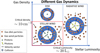 |
Fig. 1 Cartoon showing the different dynamics of the gas as a function of gas density and stellar luminosity. The critical density and luminosity showed on the figure are approximate and more precise values are presented in the paper. This paper focuses on the Stellar wind mechanism, circled in red. |
2 The analytical model
Here, we describe the gas as an idealized one-zone model with a scale height, H, and a constant density throughout for a plan-etesimal belt located between R and R + ΔR. The stellar wind velocity around M to A stars is in the range of 100–1000 km/s (corresponding to the range of escape velocities at the stellar surface, Johnstone et al. 2015a). After an elastic collision with a wind proton of velocity, υsw, at an angle, ψ, (between the proton velocity vector and the normal to the surfaces of proton and gas particle spheres at the point of contact), a gas particle of mean molecular weight, µ, will have a velocity equal to:
 (1)
(1)
provided that the initial gas particle velocity (commonly of a few km/s along the azimuth) is small compared to the end velocity after impact (see Appendix D to see the full expressions). Assuming that the wind velocity is close to the escape velocity at the stellar surface (Johnstone et al. 2015a), then we obtain the result that a gas particle will become unbound (i.e., with a velocity after impact greater than the local escape velocity) for  , assumed in our model. Indeed, for a CO molecule suffering a head-on collision, this criterion translates into R ≳ 10 R⋆ ~ 0.05 au, which will be always verified for debris disks (even a worst-case scenario of a collision with an impact angle of ψ = 89.5 deg would imply R ≳ 5 au, which will also be true as belts are typically located at tens of au).
The model we present here has been developed for systems with low gas densities where the mean free path of a wind proton, λw, crossing the belt is much greater than the belt’s width, ΔR. This means that a wind proton will (at most) interact with one gas particle in the disk (see cartoon in Fig. 1 for the basic mechanism). When λw becomes lower than ΔR, much fewer gas particles can be ejected and the density starts building up, quickly reaching the usual steady-state gas disk regime that has been described in the literature up to now (see Appendix C). The main criterion to check whether a system is in the wind regime is thus:
 (2)
(2)
If we rewrite this criterion in terms of the Knudsen number, Kn = λw/H, we obtain that Kn » ΔR/H and, thus, Kn » 1 because the scale height is much smaller than the belt width, even for the narrowest disks. For such high values of Kn, the gas will not behave like a fluid and it is mandatory to use a collisional approach to model the dynamics of the gas rather than standard hydrodynamics, as it then behaves as the sum of all individual particles.
The mean-free path of a wind proton crossing the gas in the belt can be defined as a function of the gas density, ng, and its elastic cross-section, σcol, as
 (3)
(3)
where  depends on the particles that are considered to collide with each other. We find that Rcol depends on the species considered. For an ionised species such as CO+ or C and O neutral atoms, it is roughly equal to the radius of the species considered, namely, ~0.78 Å (Miller & Bederson 1978; Olney et al. 1997) or a cross-section of ~2 × 10⁻²⁰ m2 (see Appendix B). Considering CO, the elastic cross-section with a high-velocity proton is ~2 × 10⁻¹⁸ m2 (Niedner-Schatteburg & Toennies 1992; Dhilip et al. 2006), which leads to Rcol ~ 8 Å. Solving for Eqs. (2) and using (3) to find the critical gas density, ncrit, below which the gas is in the wind regime, leads to a gas density of:
 (4)
(4)
which can also be expressed as:
 (5)
(5)
where αX is the polarisability of species X (see Appendix B) and we assume that Rcol is in the limit where its radius is fixed by the particle radius (case where collisions happen with ions or C, or O). In the case of protons colliding with CO, ncrit is 100 times smaller. In general, we find that proton collisions mostly happen faster than ionization of the gas released in the belt (see Appendix E). Indeed, for a wide range of host stars, interstellar radiation, and also accounting for SW proton ionization, we find that the ionization timescale is (most often) at least ten times greater than the time for a gas particle to get hit by a proton at the density levels we consider here (see Fig. E.1). Therefore, it is most likely that collisions will happen mainly among stellar protons and neutral atoms (e.g., C, O) or molecules (e.g., CO), but this should be checked on a case-by-case basis. We note that it also means that a CO gas disk could be above the critical density, however, after ionization of the molecules, CO+ behaves as a wind because of its much smaller cross-section; hence, this is why the most constraining value of the critical density is not necessarily that for CO collisions. The ionization of O and CO can
also happen through charge exchange with SW protons with a cross-section of σexc ~ 1.3 × 10⁻¹⁹ m2 (Izmodenov et al. 1997; López-Patiño et al. 2017). Comparing the charge exchange ionization timescale (which dominates over stellar ionization) to that of the collisional timescale for CO, we find that the order of magnitude for the ionization fraction of CO is on the order of 0.1.
Now, we define a stellar wind proton mass-loss rate, Ṁsw, and a gas production rate in the disk, Ṁg. In the case where λw » ΔR, each proton hits ΔR/λw« 1 gas particles as it passes through the disk. The number of protons (of mass mp) entering the disk per unit time is then given by Ṅp = (Ṁsw/mp)(H/R). Therefore, the number of gas particles hit per unit time is Ṅg = Ṅp(∆R//λw). If we assume that we are at a steady state and that, in addition, each gas particle exits the disk instantaneously once it is hit by a proton, then Ṅg must equal the rate at which gas particles are being replenished, that is, we get Ṁg/(µmp) = (Ṁsw/mp)(H/R)(∆R//λw). From this, we find the gas density at a steady state in the wind regime, which is equal to:
 (6)
(6)
We note that nd is the density of gas in the disk, namely, with a Keplerian rotation, while the gas density in the wind moving outwards will be described as nw and their sum by ng. The transition between the wind and disk regimes is shown in Fig. 2, representing the gas disk density as a function of a variety of realistic gas input rate for different stellar mass-loss rates. The wind regime lies below the red line representing ncrit, and because nd < ncrit is in the regime of interest, we require:
 (7)
(7)
The derived steady-state density assumes that gas particles leave the disk immediately after impact, but in reality it takes a finite time, namely, tleave Then, Eq. (6) will no longer be applicable if the gas particle gets hit by another proton before leaving the belt. To find out when this happens, we calculate the waiting time before a gas particle gets hit by a proton, thit, and compare1 it to tleave, which is the time taken by a gas particle to leave the main belt after impact. We find that Eq. (6) breaks when  (see Appendix B). In this case, another condition that should be applied in Eq. (6) is thus Ṁsw < (2πR2υswmp)/(σcolH), or in more sensible terms,
 (8)
(8)
In the absence of external perturbers, a population of col-lisionally interacting particles orbiting a central body always tends to relax toward a dynamical state where relative velocities are isotropically distributed. In terms of orbital elements, this translates into 〈i〉 ~ 〈e〉/2, with i and e being the orbital inclinations and eccentricities of solids feeding the gas, respectively, so that the scale height of the planetesimals is ~R〈e〉/2 (see Thébault 2009, for more details). To further simplify our model, we assumed that H is equal to the latter and took a typical 〈e〉 ~ 0.1 value (Thébault 2009). We also assumed that Rcol is in the limit where its radius is fixed by the particle radius (case valid for collisions with ions or C or O), but the result would be otherwise 100 times smaller if we had considered CO collisions instead. The typical value found in Eq. (8) is much greater than the solar mass-loss rate of Ṁ⊙ = 1.4 × 10⁻¹⁴ M⊙/yr and should most always be true around >10 Myr old stars, even for the youngest M-dwarfs such as AU Mic; in the latter case, wind mass-loss rate estimations are in the range of 10−103 Ṁ⊙ (Plavchan et al. 2009; Chiang & Fung 2017; Sezestre et al. 2017).
We note that when Eq. (8) breaks but Eq. (7) still remains valid, it means that each gas particle scatters tleave/thit > 1 wind protons before it is ejected from the disk. As a first approximation, this is equivalent to reducing Ṁsw by a factor thit/tleave. The new steady-state density in this case would be roughly equal to  – which is indeed independent of Ṁsw.
The gas density described by Eq. (6) is that of the gas that has not yet been kicked out by SW protons and that exhibits a Keplerian velocity. The windy part density can also be derived at the belt location. The number of gas particles hit per unit time is equal to the value of Ṅg derived previously, which can then be used to derive the wind density by dividing it by the velocity of gas particles after impact and the area of solid angle of ~π2 (see Appendix D), leading to:
 (9)
(9)
We can therefore work out the ratio of gas in the wind (moving outwards spherically) compared to that in the belt (moving in a Keplerian motion) which is equal to:
 (10)
(10)
this value may become greater than 1 for large values of Ṁsw and the wind would then dominate (see Fig. 3). Typically, for a stellar wind mass-loss rate that is a few tens of that of the Sun (rather typical in young systems, Johnstone et al. 2015a,b), values of nw become greater than nd and both components are important to consider.
When Eq. (7) breaks, then the part of the disk between R and R + λw would behave as described above, while the rest of the disk beyond R + λw would behave like a standard viscous disk (with the dimensionless α value parametrizing the viscosity, Shakura & Sunyaev 1973) as described in the current literature (e.g., Kral et al. 2019) and see Eq. (C.1). The viscous spreading happens on rather long timescales (a few Myr to tens of Myr depending on α), so that we may neglect its contribution to the inner disk which reaches the previously described steady state on much smaller timescales. In reality, the transition may not be as abrupt, as shown in Fig. 2 between the two regimes (disk vs. wind), but we still expect a strong discontinuity; this is because the part of the disk that becomes thick to incoming protons will produce gas particles with outwards velocity on the order of tens of km/s, which will collide again before leaving the disk and mostly come back to their original velocity after a few collisions. Hence, collisions no longer produce escaping gas and, thus, the gas can accumulate. A numerical model accounting for collisions in a Monte Carlo fashion could describe this transition more accurately, but this is left for a future work when a sample of clear belt wind detections become available.
In summary, we are left with two gaseous populations following the interaction of the stellar protons with the gas released from planetesimals: (1) gas colocated with the planetesimal belt characterized by a Keplerian velocity, which accumulates before being hit by protons; and (2) a spherical wind traveling outwards beyond the belt with a mean velocity on the order of υSW/µ (υSW being on the order of 100–1000 km/s for M to A stars), or typically 5–50 km/s, which leads to a slow-moving spherical belt wind. We find that for λw » ΔR, all the released gas is then eventually blown out as a wind. Otherwise, only the part between R and R + λw acts as a wind and the rest behaves as a standard viscous disk (with λw quickly becoming very small compared to R). For the case of strong ṀSW when tleave/thit > 1, a wind is still expected for λw » ΔR, but the gas density will be higher than derived in Eq. (6) because less particles can be blown out given that one gas particle gets hit by several protons. All these different regimes are shown in Fig. 2. We note that if there is another belt further out releasing a substantial amount of gas, then the outward moving wind could be affected – how-ever, the details could only be captured through a more complex numerical simulation.
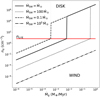 |
Fig. 2 Steady-state gas density in the belt (in Keplerian motion) as predicted by our model for different values of gas production rate. The line in red represents ncrit which is the critical density below which the gas has a wind structure (see Eq. (5)) for collisions between SW protons and either C, O, or ions. Above this critical density, the gas is assumed to form a viscous disk with α = 10−3. The case of high Msw = 105 Ṁ⊙ shows the regime where tleave/thit > 1, independent of Ṁsw where we assume υsw = 100 km/s (see main text for details). |
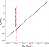 |
Fig. 3 Ratio of density between gas in the wind (spherical outward motion) to that in the belt (in Keplerian motion in the belt), at the belt location, R, as a function of the stellar wind mass-loss rate. For this plot, we use Eq. (10) with µ = 28, υsw = 100 km/s, R = 100 au, ΔR = 50 au, σcol = 2 × 10⁻¹⁸ m2, and H = 0.05R. For a stellar wind mass-loss rate that is a few tens of that of the Sun, values of nw become greater than nd and the wind becomes dominant. |
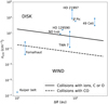 |
Fig. 4 Critical density ncrit vs. the belt width ΔR. Lines represent the critical density ncrit at which the gas transition from a disk to a wind vs. ΔR. The solid line is for a model where ncrit is given by Eq. (5) and assumes that protons collide with ions, C or O. The dashed line is for collisions between protons and CO. We indicate in capital letters whether the gas would be more DISK- or WIND-like in different regions of the plot. We note that under the black lines, winds are very likely to behave as stated in the main text. The blue points show the gas density nd estimated for the different systems shown in the plot. A vertical line joins two blue dots when a range of values are given in the literature for the gas densities or masses. Data are given in Table H.1. |
3 Results
3.1 Application of our model to real observations
We go on to use our model to compare nd and ΔR obtained from observations and investigate whether they lie at the top or bottom of the ncrit prediction, given by Eq. (4). In Fig. 4, we show ncrit as a function of ΔR, where we assumed ions, C, or O (solid) and CO (dashed) colliding with protons.
We considered a sample of observed disks with gas (described in Table H.1), which includes both high gas-density systems and low-density ones (such as the KB, for which the gas density is taken from Kral et al. 2021). Above the black solid line, the gas will always have a disk-like structure (except for very early-type stars because of the effect of radiation pressure, as explained later). Below the black solid line, a gas wind may form for the ionised, C or O gas species and below the dashed line for neutral CO gas. In Appendix E, we show that the ionization timescale tion of the gas is in most cases greater than the collisional timescale, thit, between neutrals and protons from the SW, so that gas does not ionize fast enough before it leaves the disk (except in bright FUV star systems or with strong winds) and the ionized part will start appearing at larger distances.
In Fig. 4, we notice that the gas in Fomalhaut, TWA 7, and NO Lup (all detected with ALMA) possibly lies in the WIND region of the parameter space given uncertainties. For NO Lup, a wind was recently detected (Lovell et al. 2021). For TWA 7 and Fomalhaut, the current gas detections were obtained after integrating in frequency and thus we cannot rule out a wind with full certainty. Deeper images could lead to the first confirmation of a belt wind detection. Given TWA 7 is younger, it may be favourable, but Fomalhaut would offer the first possibility to measure the stellar wind properties around an A star.
ALMA has the power to probe this “windy” domain and the deep images of ALMA targeting systems with low levels of gas could show a wind structure (i.e., gas moving radially outwards at high velocities). For instance, NO Lup is a young K7 class III system with a ~22 km/s outflowing wind detected in CO and it appears to lie right at the edge of the wind-disk transition (Lovell et al. 2021). Our model could provide the first explanation to this unexpected observation. NO Lup could be in a late T-Tauri stage2, where stellar mass-loss rates would be on the order of 10−10 M⊙yr or slighter greater (Hartigan et al. 1995), explaining why the wind would dominate over the gas in Keplerian motion (i.e., nw/nd > 1, see Fig. 3); however, observations at higher resolution are needed to confirm our hypothesis. The age of NO Lup is not very well constrained because of the unknown membership to either Lupus or Upper Centaurus Lupus, although it could be around 1–3 Myr (Lupus) or 12–15 Myr (UCL), (Luhman 2020). We note that in the T-Tauri case, we expect CO+ to dominate (which is possible if ionization is faster than the time to escape the disk in young T-Tauri stars, Heays et al. 2017), since a wind would not be present otherwise. The observed CO would then only come from recombination, which could be tested with ALMA. For more typical lower stellar mass-loss rates if CO impact ionization is faster than UV photodissociation and CO+ wind removal is faster than recombination, then we would expect CO+ to be ~0.1 times as abundant as CO in the wind (see Appendix E). Given their similar energy levels, but much stronger transitions for CO+ compared to CO, we expect CO+ J = 3−2 to be brighter than CO J = 3−2 by a factor of ~60 for similar excitation conditions. We therefore indicate CO+ as a potential tracer of disk winds around young main sequence stars.
In the β Pic system, atoms such as Ca, Na, and Fe are detected at large distances from the star going from ~10 to 100s of au (Brandeker et al. 2004; Nilsson et al. 2012). The atomic gas is in Keplerian rotation, which is surprising because it is expected that radiation pressure should blow out most atomic gas (such as FeI or FeII) on hyperbolic orbits. Brandeker et al. (2004) explain that a braking agent may be at work but that hydrogen does not work. Fernández et al. (2006) suggested a few years later that the overabundant ionized carbon may be the braking agent, which would explain the observations. In the context of this paper, we may also wonder whether stellar winds could also be important in pushing these metals away from the star where they are assumed to have been produced (e.g,. via outgassing exocomets Kiefer et al. 2014). Using the mapping of Fe I in β Pic at the VLT by Nilsson et al. (2012), we get an estimate of the Fe density at 20 au (their Fig. 9) and find ~0.2 cm−3. Given this value is smaller than the critical density found in the paper, we could imagine that (indeed) Fe or other metals could be pushed outwards due to collisions with stellar protons, in the case where the total metal density (including all species) is not greater than the critical density. However, we would need to look for the specific metal-proton cross sections in their neutral and ionized states to carry out the calculations properly, as well as the initial velocity vectors of those metals, which goes beyond the scope of this wind pioneering paper. Qualitatively, we note that when the metals enter the main gas disk in Keplerian rotation (made of CO and carbon, Dent et al. 2014; Cataldi et al. 2018) at >50 au, the total density may suddenly increase to a value > ncrit, and the metals start to brake naturally by bouncing onto other gas species (in a fluid regime); thus, they would no longer be affected by stellar wind protons. This scenario needs to be studied in more detail and comparisons to observations should be carried out to see whether it may be a competing or parallel scenario to that of radiation pressure in explaining the presence of metals located at great distances from the star in the ß Pic system. If the scenario is proven to be realistic, then observations of metallic gas winds would be expected in systems with exocomet-like detections (even around stars providing low radiation pressure) and the wind would turn into a stable Keplerian disk – if there is a susbtantial gas disk located further away.
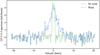 |
Fig. 5 Simulated spectra of the J = 3−2 CO line for TWA 7 for the no wind case (solid), and wind (dash-dotted) cases. Along with the moment-0 image of the disk, one can identify that the wind profile is not Keplerian but it is even more clearly visible on the moment-1 images in Fig. 7 (because the velocity structure changes significantly). |
3.2 Detecting a belt wind
3.2.1 ALMA
We go on to explore in more detail the conditions under which ALMA could clearly distinguish between a disk or a wind structure. In Fig. 5, we show simulated ALMA spectra for an observation of the gas in TWA 7 for different scenarios: a) a purely Keplerian disk or b) a wind with a velocity of 20 km/s. The υg = 20 km/s belt wind would be roughly produced from a stellar wind of velocity ~µυg of 560 km/s (not atypical for an M-star) assuming a CO-dominated wind.
For our synthetic observations, we assume that CO has a constant number density radially between 60 and 90 au, and a (radially constant) scale height of 6 au. The velocity field of this component is assumed to be in Keplerian rotation around a star of 0.51 M⊙, similarly to TWA 7. For the wind component, we assume that its density, nw, simply follows nw/nd = 0.1 at the disk location (worst-case scenario). In the analytical model we developed, we did not extrapolate our results to large distances. This is because after a collision with a proton, a gas particle can be ejected in any direction along a half sphere, whose boundary is set by the plane perpendicular to the proton velocity vector, which we call the half sphere of influence. Therefore, the emerging wind becomes 3D and it moves spherically outwards, which makes it difficult to follow analytically. Nevertheless, we developed a semi-analytical method to predict what the density and velocity of the wind will look like further away, so that we are able to make accurate predictions for the observations (see details in Appendix G). The results are shown in Fig. 6, presenting the (from top to bottom) face-on and edge-on densities and the velocity structure.
The velocity profile we derived will be used to mimic the expected doppler profile of the gas wind to make synthetic images. As can be clearly seen in Fig. 6, the gas outflow has a butterfly-like shape in the edge-on direction, with its density peaking along the direction of the disk mid-plane. In the head-on direction, it logically assumes an isotropic profile that continuously decreases outward. As for the orientations of mean velocities within the outflow, they schematically radiate from the location of the parent belt, while the absolute magnitude of the velocities is maximum in the prolongation of the belt’s mid-plane. This is an expected result as this is the direction for which the kinetic energy transferred by the impacting protons is at maximum (see Eq (D.1)).
For building the synthetic images, we also assume a ~1′′ resolution corresponding to ALMA in its most compact (C-1) configuration, which gives a ~40 au resolution at TWA7’s distance. We find that we can distinguish between a purely Keplerian disk model and a wind model for a sensitivity of 1.5 mJy beam for a spectral resolution of 244.14 kHz (corresponding to a velocity resolution of 0.21 km/s), which requires roughly 5 hours on source with 43 antennas. The 20 km/s wind can clearly be distinguished because of its wider non-Keplerian spectrum when compared to the gas position given by moment-0 images (see Fig. G.1). Moreover, in Fig. 7, we show the moment-1 velocities (intensity-weighted velocity) for the different scenarios and find that the wind case can clearly be distinguished from the no-wind case given their very different radial velocity structures. In the case of the 20 km/s wind, the velocity is perpendicular to the position angle of the disk (that is obtained thanks to optical observations for the case of TWA 7, Olofsson et al. 2018), while it is aligned with it for the no-wind case, which is also clear on the position-velocity diagrams (see Fig. 8).
We may thus conclude that from these types of observations, we could clearly distinguish “belt” winds with ALMA and use them to access to the SW velocities and densities around main-sequence stars, which is otherwise difficult (Johnstone et al. 2015a).
Indeed, from the detection and using Eq. (6) with ndobs (the observed disk density), we can go back to the factor Ṁg/ṀSW. If the wind is detected then we can use the simple one-zone model presented in the paper to get some first estimates of the stellar wind velocity assuming that υsw ~ µ〈υwobs〉 (the mean value of the observed wind velocity derived from the redshift of the wind compared to the star velocity and after correcting for potential orientation effects). We can also retrieve a value of Ṁsw, which does not depend on Ṁg (hence, it is independent of a gas-release model) using Eq. (10), that is, by computing the ratio between nwobs (the observed wind density) and ndobs In Appendix F, we describe the process in greater detail.
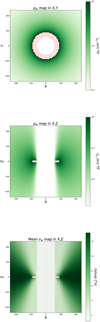 |
Fig. 6 Wind structure for a belt extending from 60 to 90 au. Top: wind density in a (X, Y) plane at Z = 0 (cut in the midplane). The density was set to 1 cm−3 for the wind emerging from the belt. Middle: wind density in a (X, Z) plane at Y = 0 (cut at the middle of the belt). Bottom: velocity structure (direction and magnitude) integrated along the line of sight (assumed here to be along the Y axis). The red hatches show the location of the belt that releases gas. |
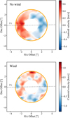 |
Fig. 7 Moment-1 images (intensity-weighted velocity) for the no wind (top) and wind (bottom) cases. The no-wind Keplerian case is aligned on the disk position angle while it is very inclined or even perpendicular for the wind case, making them easily distinguishable, which can also be seen on the position-velocity diagram (Fig. 8). |
3.2.2 In the UV or optical
Observations of those winds may also be possible in the UV, as implied by recent detections of a gas wind in η Tel (Youngblood et al. 2021). However, the feasibility of far-UV absorption studies from space relies on two factors. The first is the viewing geometry of the wind, which needs to cross the line of sight and produce a sufficiently high column density for detection. As shown in this paper, the column density would be highest through the disk midplane, thus favoring an edge-on viewing geometry. However, we note that if the wind density is high compared to that of the disk (in Keplerian rotation), there is more leeway on the inclination because even for a face-on geometry, some gas particles will still cross our line of sight since they can be ejected perpendicular to the midplane. The second factor is the presence of a strong, detectable background, which is typically the central star. However, the star’s flux density at the relevant UV wavelengths (~ 1500 Å for the main CO A–X bands, see e.g., Roberge et al. 2000) is on the Wien side of the stellar emission and, therefore, very strongly dependent on the spectral type, distance from Earth, and the presence of UV excess, if any. As the viewing geometry and stellar flux density are very system-specific, it would be difficult to make a prediction on whether winds could be generally detectable at UV wavelengths or not. A more promising and widely-applicable avenue could be detection of CO+, as is common for Solar System comets, in the violet region of the optical (~4200 Å A–X bands, e.g., Cochran & McKay 2018). Absorption studies in this range would benefit from a much improved strength of the stellar continuum, allowing a wider range of spectral types and distances from Earth to become accessible. The CO+ bands are however complex, and would require a specific line list with adequate codes to handle the radiative transfer. We therefore deem a thorough exploration of a CO+ detection in an exoplanetary system in this wavelength range to be beyond the scope of this paper.
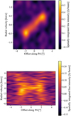 |
Fig. 8 Position-velocity (PV) diagrams for the no wind (top) and wind (bottom) cases. The no-wind Keplerian case shows a typical PV diagram for a Keplerian disk along its position angle while it is horizontal for the wind case, making them easily distinguishable. |
3.3 Predictions of debris disk systems with belt winds
Finally, we assess how to predict a gas wind presence from dust observations of debris disks only (which are much more numerous than that of gas) and, more specifically, from their fractional luminosity (the infrared luminosity over that of the star) as well as their stellar luminosity. These are data that are accessible for hundreds of debris disks (see details in Appendix C). To carry out this assessment, we assume that gas is injected in the belt at a rate, Ṁg, and then evolves viscously with an α prescription (Kral et al. 2016; Kral & Latter 2016). We assume that the gas disk reaches a steady-state and compare the gas density to ncrit to find when the gas density becomes so low that gas starts behaving as a wind. It leads to Eq. (C.6), which can be further simplified to:
 (11)
(11)
where f is the fractional luminosity of a debris disk and L⋆ is the host star luminosity. We use this equation and the fiducial values used in it to make Fig. 9, which shows the DISK versus WIND regions for varying f and L⋆. Therefore, a wind-like structure is expected for disks with low fractional luminosities, on the order of 10−5–10−4 for M stars and down to 10−6–10−5 for the more massive A stars. It shows that late type stars are expected to create gas winds more readily than, for instance, A-type stars.
However, for A stars with overly high luminosities, namely, L⋆ ≳ 20 L⊙, a gas wind is also expected because of the radiation pressure becoming too high on the gas as was shown in Fig. 11 of Kral et al. (2017), and more recently by Youngblood et al. (2021), with a criterion on the temperature such that T⋆ > 10 200 K. We note that when the gas starts becoming optically thick to UV photons, this mechanism would stop working (Kral et al. 2017), which needs to be computed for each observation. Indeed, Kral et al. (2017) predicted that in all systems with ṀCO > 10−4 M⊕ Myr−1 , ionised and neutral carbon can be protected from being blown out thanks to shielding. Without shielding, ionised carbon would be blown out for systems with L⋆ > 15 L⊙ but neutral oxygen would stay bound up to 25 L⊙. This region of the parameter space with low fractional luminosities is expected to be the most populated by population synthesis models of debris disks for A stars (Wyatt et al. 2007) and for F, G, and K stars (Sibthorpe et al. 2018). We note that Eq. (11) gives an order of magnitude because the gas density derived from the standard gas disk model we use may not be an exact good fit of observations for a specific system (and α could vary). Thus, debris disks with slightly larger fractional luminosities such as TWA 7 or Fomalhaut can still be in the WIND regime because gas observations show that they indeed have low gas levels.
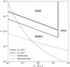 |
Fig. 9 Transition between disk and wind regions shown in the space of the fractional luminosity of a debris disk as a function of the host star luminosity. The bottom left and far right regions are likely to be populated by gas having a wind structure while the upper left region would more likely be filled by circumstellar gas disks. We show the limit between disk and wind cases for two values of α: 0.1 (solid) and 0.01 (dashed). The thin red and blue lines are dust detection limits of ALMA at 870 microns and Herschel at 70 microns assuming dust lies at 100 au. See the assumptions behind this plot at the end of Appendix C. |
4 Conclusions
In this paper, we explore whether the gas that has been detected in many debris disk systems may be blown out as a wind due to collisions with high-velocity protons from stellar wind, rather than being a circumstellar disk in Keplerian rotation, as assumed in current models. We find that, indeed, this wind-like behaviour of the gas might be present in systems in which the gas density is low, typically below the threshold value of 7 (ΔR/50 au)−1 cm−3, where ΔR is the belt's width. We find that the analytical model we developed may explain the outflowing gas detection in the young NO Lup system. Moreover, the two systems with the lowest gas masses detected to date, TWA 7 and Fomalhaut, may already be in this wind region and further observations with ALMA could clearly disentangle any uncertainty between a disk and a wind structure. More generally, we find that debris disks with low fractional luminosities such that f ≲ 10−5(L⋆/L⊙)−0.37 are naturally expected to form “belt” winds. Likewise, gas is expected to have a wind-like structure around early type stars with luminosities ≳20 L⊙ because of the action of radiation pressure rather than stellar wind (see the cartoon in Fig. 1 illustrating all the different gas dynamics expected for varying gas densities and stellar luminosities). In addition, we argue that gas released very close to the central star by, for instance, FEB-like bodies (falling evoparating bodies or star-grazing exocomets) could also be affected by stellar winds and may explain some observations in the β Pic system or lead to further interesting detections around systems with detected FEBs. We find that CO+ may be a good tracer of belt winds created because of the action of stellar winds and it can be targeted with ALMA and probably in the optical. Future detections of belt winds would allow us to retrieve the SW properties (mass-loss rate and velocity) around a broad variety of MS stars, which are otherwise difficult to measure – especially around A stars where no measurements have led to any detections thus far.
Acknowledgements
This paper is dedicated to Florian. We thank the referee for a helpful review that improved the quality of the paper. Q.K. thanks Hervé Beust and Alex de Koeter for interesting discussions about induced dipole interactions and stellar mass-loss rates, respectively. Q.K. also thanks Alexandre Faure and Evelyne Roueff for discussions about elastic cross sections.
Appendix A Stellar wind model
In this work, we are primarily interested in stellar winds produced around both young and old stars, for spectral types going all the way from A to M (O and B stars are not considered here). Stellar wind measurements are scarce (~ 12 systems) around MS stars because they are difficult to detect (Cranmer & Saar 2011). For A stars, there are no detection so far and the mechanism behind their winds still needs to be assessed firmly (Lanz & Catala 1992; Krtivcka 2014).
There are two fundamental properties for SWs: their velocity, υsw, and density, nSW, (linked to the stellar mass-loss rate, Ṁ⋆). To assess the values of those properties, we use models, such as that of Johnstone et al. (2015a), which describe SW properties for dwarf main-sequence stars (M, K, G, and F type stars). This model is an extension of a state-of-the-art Solar wind model. The mechanisms that heat the solar corona and accelerate the solar wind remain unknown to this day. The two main competing hypotheses are that the solar wind could be driven by the dissipation of Alfvén waves and turbulence, or by magnetic reconnection events (e.g., Cranmer & van Ballegooijen 2010). In a similar way, many uncertainties remain about winds around main-sequence A stars that cannot be probed easily. Theoretically, no significant winds are expected for stars with spectral types later than B6, for which the line-driven mass-loss rate should be smaller than 10−12 M⊙/yr (Krtivcka 2014). An empirical upper limit is reported in Lanz & Catala (1992), leading to a less constraining value of 1 − 2 × 10⁻¹⁰ M⊙,/yr. There could be other mechanisms than line-driven winds driving stellar mass loss in A stars (e.g., magnetism, pulsation, coronal heating), but only observations could provide more insights. If none of these mechanisms can drive winds efficiently in A stars, then the mass-loss rate could even be smaller than for our Sun, that is, < 1.4 × 10⁻¹⁴ M⊙/yr. Winds around O- and earlier B-type stars are more powerful and are expected to lead to higher velocities and densities, but they are not considered in this study because the number of debris disks found around these stars are only a handful. Winds around younger T-Tauri or Herbig stars are also expected to be larger, reaching values greater than 10−10 M⊙/yr (Hartigan et al. 1995; Nisini et al. 1995).
As it is noted in these models, there are large uncertainties on the properties of the SWs around stars of A to M spectral types, and we will explore a large range of values to account for that. The wind velocities can roughly vary from 100 to 1000 km/s (it is close to the value of the escape velocity at the star surface) and the stars’ mass-loss rates on the MS can go from 0.1 to 1000 that of our Solar System where Ṁ⊙ = 1.4 × 10⁻¹⁴ M⊙/yr, and greater for even younger stars on the pre-main sequence. For instance, for the emblematic AU Mic system, theoretical estimates for the stellar mass-loss rate varies from 10 (Plavchan et al. 2009) to 1000 Ṁ⊙ (Chiang & Fung 2017; Sezestre et al. 2017).
From the stellar mass-loss rate, we can then find the SW density used in this paper through the relation that follows:
 (A.1)
(A.1)
with µw = 0.6, the mean molecular weight of the wind, based on the Solar wind (Johnstone et al. 2015a) and we use the notation ṀSW (instead of Ṁ⋆) when only accounting for protons from the stellar wind in the main text and then take µw = 1 in the previous equation to get the stellar wind proton density.
We note that the star mass-loss rate depends on the star radius and mass, as well as the stellar angular velocity Ω⋆, and scales as  (Johnstone et al. 2015a), so that the Solar wind was predicted to be an order of magnitude stronger in its youth and more generally, young systems are expected to have stronger SWs because of the faster rotation of the central star (Johnstone et al. 2015b). The angular velocity of main-sequence stars can vary but is highest between 10-100 Myr and can reach 100 Ω⋆, with a mean of ~ 10 Ω⋆ for solar type stars and low-mass stars (Bouvier 2013). As a first approximation, the angular velocity scales with time as t−1/2. Our model also accounts for saturation effects, namely, there is a limit at which mass-loss rates can increase due to an increase of Ω⋆, happening at Ωsat = 15Ω⊙(M⋆/M⊙)2.3, where Ω⊙ = 2.67 × 10⁻⁶ rad/s is the Carrington rotation rate. We use this SW model in Appendix E to work out typical SW collisional timescales.
Appendix B Belt wind model
Here, we describe an idealized belt wind model for a planetesimal belt comprised between R and R + ΔR with a scale height H and a constant density throughout. The gas producing the belt wind is released from planetesimals (e.g., by collisions or sublimation, Kral et al. 2021) and then pushed outwards by impacting stellar wind protons. We first describe the regime where the rate of gas production is small relative to the stellar wind, namely, it is the case described in Kral et al. (2021) for the Kuiper belt, where all gas particles get hit and ejected outwards by the stellar wind, thus creating a belt wind.
We then define a wind proton mass-loss rate ṀSW and a gas production rate in the disk Ṁg. We assume that the mean-free path of wind protons in the gas λw = 1/(σcolng) is much greater than the belt’s width ΔR, where σcol is the proton-and-gas particle collision cross-section.
For instance, in the case of ion collisions (e.g., C+ colliding with protons), we expect the elastic cross-section to be small because charged particles are repulsive at long range. To quantify that, we use that the kinetic energy of the proton equals its electrostatic energy to get:
 (B.1)
(B.1)
where e is the elementary charge, є0 the vacuum permittivity, mp the proton mass, and υcol the relative velocity between ions and protons. We find that for typical velocities > 100 km/s, Rcol becomes smaller than the typical radius of ions so that we should use the radii of ions instead. We thus take Rcol ~ RX, where RX is the typical radius of the particle modeled by an imaginary hard sphere (Van der Waals radius) given by (3αX/(4π))1/3. We take αC0 = 1.953 Å3, αC = 1.760 Å3, and αo = 0.802 Å3 (Miller & Bederson 1978; Olney et al. 1997) and will use αCO in our fiducial model. This leads to RCO ~ 0.78 Å or a collision cross-section of ~ 2 × 10⁻²⁰ m2.
For collisions between protons and CO, we use the assumption that the elastic cross-section with protons at 30-100 eV is ~ 2 × 10⁻¹⁸ m2 (Niedner-Schatteburg & Toennies 1992; Dhilip et al. 2006); typically, this is Rcol ~ 8 Å.
For collisions between protons and neutral C or O atoms (which have no permanent dipoles like CO), we use the assumption that the proton induces a dipole on the neutral atom so that (Beust et al. 1989; Beust & Valiron 2007):
 (B.2)
(B.2)
where αX is the polarisability of species X, υcol the relative velocity between protons and neutrals, and mred is the reduced mass of the two colliders approximately equal to mp, the proton mass, when a proton collides with a more massive neutral. When Rcol becomes smaller than the actual radius of the particle, we use the latter instead. For a typical wind speed greater than 100 km/s, we thus take Rcol ~ RX, where RX is the typical radius of the particle. This leads to RCO ~ 0.78 Å or a collision cross-section of ~ 2 × 10⁻²⁰ m2 similar to that of ions.
In the case that λw » ΔR, the reasoning in the main text follows along to the conclusion that the gas density at steady state in this regime is:
 (B.3)
(B.3)
and the assumption we made that λw » ΔR, together with Eq. B.3, leads to
 (B.4)
(B.4)
so that when the proton wind rate becomes too small or the gas production rate too high, the steady-state gas density calculated above needs to be changed (see later). To give an idea of the contribution of the wind with a spherical outward motion compared to gas in the belt in Keplerian motion, we plot nw/nd as a function of ṀSW in Fig. 3. We note that the wind profile (density and velocity) at large distances from the belt is also computed in Appendix G so that we are able to make predictions for future ALMA observations.
When computing the steady-state above, we assume that once a gas particle has been hit by a stellar proton, it leaves the disk immediately, which may not be true if the time to leave the disk after impact tleave becomes much longer than the time thit before a gas particle gets hit by a proton once it is released from a planetesimal. We calculate that thit = 1/(nSWσcolυSW). The gas particle and the proton typically undergo a large angle collision and the post-collision velocity is roughly isometric (see Appendix D), so that most particles will travel less than 2H before leaving the disk. The mean speed of the gas particle after the collision with a proton is given by υɡ ≈ υSW/µ. We may thus estimate tleave = µ(2H/υSW) and get:
 (B.5)
(B.5)
Equation B.3 is valid as long as tleave/thit < 1 and breaks when this ratio becomes > 1, which corresponds to ṀSW > (2πR2υSWmp)/(σcolH). In this case, and if we also have ṀSW > (Ṁg/µ)(R/H) to account for Eq. B.4, we expect that the particles are hit multiple times by different protons before leaving the disk thus reducing the wind efficiency to eject gas particles (e.g., two protons only eject one gas particle instead of two). The gas density that accumulates between R and R + ΔR will be nd(tleave/thit), with the fraction in parentheses accounting for the reduced efficiency of the proton wind to blow gas particles out. Thus, we find in this regime that:
 (B.6)
(B.6)
which is independent of ṀSW.
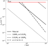 |
Fig. B.1 Steady-state gas density in the belt predicted by our model as a function of r, which is the radial distance to the star. The fiducial model has a = 1, b = 0, R0 = 100 au, h0 = 0.05, ṀSW = 1.4 × 10⁻¹⁴ M⊙/yr, and Ṁg = 10−3 M⊕/Myr (see Eq. B.7). Values below Rcrit (see Eq. B.8), i.e., above the red line, are not shown. The density beyond the planetesimal width ΔR will mostly scale as r−2 as the fiducial model (see Appendix G) but it is not represented in the plot. |
If we now assume that the gas surface density is not constant but given by Σ = Σ0(r/R0)−a and H/r = h0(r/R0)b, then following the same procedure as described before to find the steady-state but using dr annuli instead, we find that nd = Σ/(2Hµmp) can be defined as a function of its radial distance r as follows:
 (B.7)
(B.7)
where Σ0 = (Ṁg/ṀSW)(2mp/σcol)(R0/ΔR). We plot nd(r) in Fig. B.1 for various values of a, b, ṀSW, and Ṁg. We note that in this case, there is a minimum radius Rmin below which nd(r) can become greater than ncrit (the critical gas density below which a gas wind forms, see Eq. 4) and in this case, the gas would become optically thick to protons and the gas structure would be disk-like. To avoid this, Rmin should remain greater than:
 (B.8)
(B.8)
assuming that ΔR ≲ Rmin, otherwise it gets more thorough to work out. We also note that beyond the planetesimal belt of width ΔR, the gas wind density will mostly scale as (r/R)−2 (see Appendix G), assuming that the rate of collisions with stellar protons becomes negligible.
Appendix C Gas model and comparison to ncrit
Here, we describe the standard gas disk model we use to make a comparison with ncr¡t and to find the range of debris disk global parameters that will populate the DISK versus WIND regions in Fig 9. For a disk of scale height, H, and mean molecular weight, µ, the gas density can be linked to the gas surface density, Σɡ(r), as follows
 (C.1)
(C.1)
and the surface density for a disk located at R0 where gas is input at a rate of Ṁg is equal to (Kral et al. 2019)
 (C.2)
(C.2)
where  is the viscosity at R0 and the temperature scales as T ∝ R−γ. We note that in this case, ng scales as R3γ/2–3 for r < R0, and as R3γ/2–3/2 for r > R0 at the steady state.
Now, we want to find when ng = ncrit so that we can see which parts of the parameter space will fall in the DISK versus WIND regions. As a first approximation, we compute the gas density at R0 to compare it to our one-zone model critical density (Eq. 4) and after rearranging the equality, we find:
 (C.3)
(C.3)
which gives the order-of-magnitude gas-production rate where there is a change of regime from a disk to a wind structure.
To relate the debris disk properties (e.g., luminosity, radius) to the previous equation, we use the fact that the gas input rate is related to the mass-loss rate of the belt (Kral et al. 2017) through
 (C.4)
(C.4)
where  , with ξ as the ratio of gas-to-dust mass-loss rates and assumed to be on the order of 10%, f as the fractional luminosity of the debris disk, L⋆ as the stellar luminosity (in L⊙), e as the mean eccentricity of the parent belt planetesimals, dr as the belt width (in au),
  as the collisional strength of solids (in J kg−1), and ρ as their bulk density (in kg/m3). Using the same typical values as in Kral et al. (2017) for e, dr,
  and ρ, we find δ = 2.9 × 10⁴.
As we are interested in the limit between DISKS and WINDS for neutral or ion collisions at high velocity (>100 km/s), we use the following:  , with Rcol is set to the CO radius (case for collisions between CO+, C, or O, and protons). We then find that the condition for planetesimal-generated gas to assume a disk-like structure is expressed as:
 (C.5)
(C.5)
where we assumed  .
.
Moreover, if we assume the empiric law derived by Matrà et al. (2018b) showing that the radial location of a debris disk peak density varies with stellar luminosity following R0 = 73au (L⋆/L⊙)0.19, then Eq. C.5 can be simplified to:
 (C.6)
(C.6)
For gas in debris disks, α values could be very high (of order 0.1) because of the high ionization fraction in these disks that may give birth to a strong magneto-rotational instability (MRI, Kral & Latter 2016). Indeed, fitting of the current gas observations favour high a values on the order of 0.1, as shown in Kral et al. (2019); Marino et al. (2020). However, smaller values could also be realistic because non-ideal MRI effects may start being important at low gas densities (e.g., α = 10−4) and observations of such disks in the future may allow these aspects to be probed more clearly.
Appendix D Collision outcome between a wind proton and a gas particle
An elastic collision between a proton of initial velocity, υp, and position, rp, with a gas species, X, of initial velocity, υX, and position, rX, will lead to a post-collision velocity  for the species, X, given by:
 (D.1)
(D.1)
and for the proton
 (D.2)
(D.2)
where µ is the mean molecular weight of the gas particle being hit by the proton.
Given that the proton velocity is much higher than that of the gas particle, and further assuming that the proton moves radially with ||υp|| = υSW, the equation for  can be simplified to 2υSW cos(ψ)/(µ + 1), where ψ is the collision angle (shown in Fig. D.1). Assuming that the two particles are two spherical balls, the collision angle is roughly given by the angle between the proton velocity and the normal to the surfaces of balls at the point of contact (ψ = 0 for a head-on collision and π/2 for edge-on) and
  is parallel to the normal to the surfaces of balls at the point of contact. The angle ψ can vary between [0, π/2] and after a collision with a proton, the gas particle most likely exits the disk via its vertical height rather than crossing its whole belt of width ΔR > H. We note that there will be fewer collisions with ϕ angles close to π/2 because higher impact angles cover fewer impact parameters that are uniformly distributed. The distribution of impact angles scales as cos(ϕ), meaning that the impact angles are well represented by a cone pointing radially outwards with an opening angle ϕm of ~ 50 deg (since nearly 4/5 of collisions will occur in that cone). We deduce that the molecules escape into a solid angle of approximately 2π × 2ϕm ~ π2.
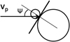 |
Fig. D.1 Schematic of the collision between a proton of initial velocity υp with a gas particle. The collision angle ψ is between the normal to the surfaces of the spheres at the point of contact and the proton velocity. |
Appendix E Ionization timescales
Carbon can be ionised by energetic (>11.26eV) photons from the ISM on a timescale of roughly 120 yr (Visser et al. 2009), which corresponds to a photoionization rate of 3 × 10⁻¹⁰ s−1. Carbon, oxygen, and CO can also be ionized by stellar radiation, as is the case in our Solar System, where the photoionization rate is 5 × 10⁻⁷(1 au/r)2. The ionization of O and CO can also happen through charge exchange with SW protons with a cross-section of σexc ~ 1.3 × 10⁻¹⁹ m2 (Izmodenov et al. 1997; López-Patiño et al. 2017), which translates into an ionization rate of 1/tion = nswσexcυsw, where tion is the ionization timescale (see Appendix A for the details of the SW model we used). This is roughly an order of magnitude smaller than the collisional timescale for CO meaning that some CO+ may appear even in CO dominated-regions with a factor one to ten in density. We also used spectra from Castelli & Kurucz (2003) to get typical stellar fluxes F (in erg/s/cm2/nm) for different stellar types and ionization cross-sections σi (in cm−2) from Heays et al. (2017) to compute the photoionization rates, px, (in s−1) for a species, X, such that  with λ the wavelength in nm and hv in erg, where most of the cross-section is in the UV.
The ionization timescale should be compared to the collisional timescale between protons and neutrals, because after one collision with a fast SW proton (≳1·00 km/s), the gas particle becomes unbound and leaves the system very quickly; this means that it rapidly reaches the outer regions (Kral et al. 2021). The collisional timescale between SW protons and neutrals is thus thit = l/(nSWσcolυsw)·
After a collision, the gas particle direction is isometric (inside of the cone that points outwards of the collision direction) and will usually leave the disk at high angles (see Appendix D), thus traveling roughly 2H before escaping the belt rather than crossing its whole length ΔR. We need to see how the time to leave the disk tleave compares to tion. The timescale for a gas particle to travel 2H of the disk given its post-collision velocity (see Appendix B) is roughly 2Hµ/υsw. It is important to calculate tleave to understand whether gas particles get ionised before or after leaving the disk.
Figure E.1 shows tion, tleave, and thit as a function of r, the radial distance to the central star. We notice that the SW collisional timescale, thit, becomes smaller with decreasing age or increasing mass-loss rate, which are both expected to be at their highest when the systems are young. We also find that increasing collision velocity will increase thit by a small amount. We see that at the typical location of debris disks (between ~30-150 au), the smallest timescales are always tleave and thit, meaning that before CO, or O have time to ionise, they are pushed outside of the main disk (unless they are already ionized when released). However we note that ionization via SW protons of CO is the most efficient and some CO+ may be present. For completion, we note that the photodissociation of CO takes roughly 120 yr at large distances from the star (owing to the ISM photons, Visser et al. 2009) and for other important timescales, we refer to Tables C1 and C2 in Kral et al. 2021. Most of the gas close to the belt is then expected to be neutral and molecular, which could ease detections with ALMA targeting CO lines.
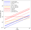 |
Fig. E.1 Timescales for ionization tion (red), leaving the disk tleave (orange), and stellar wind collisions with CO thit (blue) Vs distance to the gas. The fiducial model labeled as the “young system” has M⋆ = 1M⊙, υsw = 100 km/s, and Ω⋆ = 10 Ω⋆. The timescale tion for SW protons is shown for a young system but it is always an order of magnitude greater than thit. |
We do not rule out that for a specific very young system that is still emitting large amounts of FUV photons, the ionization timescale may become smaller than calculated here from the standard Castelli & Kurucz (2003)’s stellar spectra and, in this case, ionized species could be present as well as individual C or O atoms (which may also get ionized), rather than CO close to the belt, and CO+ may start to dominate. It could also be that in old systems the stellar mass-loss rate becomes too small and gas has time to ionize and/or photodissociate before it gets pushed away by SW protons. However, since most observations are for young systems currently, this case is not often expected but might still drive our observing strategy to detect belt winds. We still recommend that these timescale comparisons be performed when studying a specific system for assessing the state of the gas given its specific stellar spectra, angular velocity, and mass-loss rate.
Appendix F Retrieving stellar wind characteristics from gaseous belt outflows
Here, we describe how we would retrieve the SW density and velocity around main sequence stars thanks to, for instance, ALMA observations of CO or neutral carbon gas. It is important to find new techniques to do that because currently we only have a dozen of measurements for main-sequence stars (Cran-mer & Saar 2011) - but none for A stars (Lanz & Catala 1992; Krtivcka 2014).
The first thing to do is to retrieve the carbon or CO density in the belt (with a Keplerian motion) from observations (or by putting an upper limit to it if the wind dominates and hides the Keplerian component), which should be easy because in these low gas mass systems, lines are optically thin and we expect the gas to be close to the purely (non-LTE) radiative regime where the line intensity does not depend on temperature. Hence, we can retrieve the gas mass and density ndobs. If the wind (moving spherically outwards) is also detected, we can retrieve its density nwobs. In this case, we can also derive the mean gas velocity 〈υwobs〉 from the associated redshift of the wind compared to the star velocity and after correcting for potential orientation effects.
Assuming a steady state and using Eq. 6 with ndobs, we can go back to the factor Ṁg/ṀSW. If the windy part of the gas is not detected then using a model for the gas production rate, for instance, as described by Eq. C.4 (Kral et al. 2017), we can retrieve the stellar mass-loss rate, MSW. If the wind is detected then we can use the simple one-zone model presented in the paper to get some first estimates of the stellar wind velocity assuming that υSW ≈ µ〈υwobs〉. We can also retrieve a value of ṀSW, which does not depend on Ṁg (hence, independent of a gas-release model) using Eq. 10, that is, by computing the ratio between nwobs and ndobs.
The first unambiguous detection of a belt wind would have the beneficial side effect of allowing us to improve our model further. Such an improved model (which is beyond the scope of this paper) would extend our one-zone approach to a numerical multi-zone model using Monte Carlo simulations to compute the outcome of the different collisions with SW protons and reach a steady state. This could be particularly useful for resolved observations. For short collisional timescales with the SW, there could be multiple collisions before reaching the end of the SW bubble (called heliosphere in our Solar System and located at ~ 150 au, Opher et al. 2020). We could also include collisions with protons from the local interstellar medium, whose density is around 0.1 cm−3 (Izmodenov et al. 1997), when the gas reaches beyond the SW bubble. The end velocity at large distances would then be close to that of the protons from the ISM. Finally, the gas state (owing to ionization, photoionization,…) could also be followed more accurately coupling the code to a PDR-like model to make some predictions for different lines.
Appendix G Prediction of the wind profiles at large distances and observations with ALMA
Appendix G.1 Wind profile at large distances from the belt
Our approach assumes that after a collision, gas particles exit the disk and they do not get hit by another proton afterwards. First, we create a 3D cartesian grid and we refer to production cells as the space between 60 and 90 au, and with z lower than the scale height, that is, where the planetesimal belt is located. Exterior cells (or wind cells) then refer to all the other cells. Our approach is simple: each production cell (x,y,z) in the disk produces a flux of scattered molecules in a cone, directed in the radial direction. The emitted flux density and velocity of the scattered molecules depends on the angle of collision ψ we defined in Appendix D. For each exterior cell, we add the contributions, to both the wind density and its velocity distribution from all production cells whose post-collision gas outflow cone crosses this exterior cell.
In practice, we assume that the gas velocity is constant after impact with a proton and that the density decreases as  beyond the production cell, with rd being the distance between the production and the exterior cells considered. We run through each production cell and consider all exterior cells that it can target (i.e., all cells beyond the half sphere or cone of influence) and add the contribution weighted by
  to the density it had when emerging the belt. We also calculate the angle between the production and exterior cells and multiply the contribution in density by 1 / cos ψ because gas particles leaving their cells at high angles (e.g., ψ is close to π/2 for edge-on collisions with protons) will move more slowly than for head-on collisions. However, there will also be less collisions at high angles because high impact angles cover less impact parameters than low ones and we add a cos ψ contribution to account for that effect, thus canceling the previous effect. We proceed in the same way to get the contribution in velocity from all interior cells and calculate the velocity direction by computing the normalised vector between the two cells. We also weight the different contributions by the density and account for the cos ψ factor because head-on collisions will lead to a faster moving wind. We then average the different velocity vector contributions coming from all production cells and consider the final velocity vector as being representative of what a mean radial velocity offset will look like in real observations. The density and velocity fields are plotted in Fig. 6 and used to make the synthetic observations presented in the paper.
Appendix G.2 ALMA synthetic images for future observations
To make detailed predictions for detectability of a wind with future observations, we focus on the TWA 7 system and follow four steps.
First, we define the density and velocity structure of the CO disk and the wind component. For the CO disk component, we assume that it has a constant number density radially between 60 and 90 au, and a (radially constant) scale height of 6 au. The velocity field of this component is assumed to be in Keple-rian rotation around a star of 0.51 M⊙. For the wind component, we assume that its density, nw, simply follows nw/nd = 0.1 at the disk location (worst case scenario). At radii and vertical heights larger than the disk’s, we assume the density and velocity structure described at the beginning of this section.
Second, we calculate the excitation of the CO gas assuming it is out of LTE and purely in the radiation-dominated (low-density) regime. This is justified by the low densities expected in an environment largely devoid of species other than CO. At each position within our model, we calculate CO level populations using non-LTE codes including the effect of UV/IR fluorescence due to absorption of UV/IR stellar/interstellar radiation (Matrà et al. 2015, 2018a). The stellar and interstellar radiation components are as described in Matrà et al. (2019), with the stellar contribution rescaled with the inverse of the gas stellocen-tric distance. To keep our feasibility test as realistic as possible using measured line intensities, we target the same CO transition (J=3-2) detected by existing ALMA observations (Matrà et al. 2019).
Third, we use our 3D density, velocity, and excitation structure in our model to carry out radiative transfer using the RADMC-3D code (Dullemond et al. 2012). For the temperature structure, for simplicity we assume radius-dependent blackbody temperatures appropriate for the luminosity of the host star; we note that these temperatures do not affect excitation in the radiation-dominated regime, but only the intrinsic CO J=3-2 line widths. This produces a spectro-spatially resolved cube of CO J=3-2 line intensities. The output cube has a pixel size of 0.1”, extending spatially out to ±6.4” from the star. The cube has a channel size of 244.14 kHz (0.21 km/s at the line location of 345.796 GHz) and extends out to ±21 km/s from the stellar velocity. We note that we rescale the input CO mass to produce a peak CO line intensity (after spatially integrating over the entire model) of 60 mJy in a 244.14 kHz channel, to ensure consistency with the existing ALMA dataset (see e.g., Matrà et al. 2019, Fig. 1, top spectrum). This leads to a model with a characteristic CO number density of ~100 cm−3 within the disk component. We note that this is an upper limit of the density in the disk because we assumed a purely radiation-dominated regime but a few colliders could bring it closer to LTE in a regime where the gas density would not need to be as high to explain the CO detection around TWA 7. For instance, in LTE we find that a gas density of 0.08 cm−3 in the disk is enough to explain the CO J=3-2 detection. The real density therefore must line in between but our synthetic images do not change much between the two regimes because of the rescaling to get the right intensity and our predictions remain valid whatever the amount of colliders.
Finally, we produce synthetic ALMA visibilities using the simobserve task within the CASA software v6.4 (McMullin et al. 2007). Due to the low expected CO surface brightness of CO emission, we simulate 345 GHz (Band 7) observations in the most compact array configuration (C-1, baselines from 15m to 161m), leading to abeam size of 1.06” × 1.25”, corresponding to ~40 au at the distance of the star. We simulated enough repetitions to reach a cube sensitivity of 1.5 mJy/beam in every 244.14 kHz channel, a factor of 4.6 deeper than existing observations. Visibilities are imaged to produce line cubes using the tclean CASA task, using natural weighting and standard Hogbom deconvolution. To produce moment-0 images (Fig. G.1), we spectrally integrate the cube over velocities where the CO J=3-2 line is significantly detected (±6.7 km/s), whereas to produce 1D spectra we spatially integrate in a radial region between 1.2” (40 au) and 3.2” (110 au) from the central star. Finally, to produce moment-1 maps (Fig. 7), we select the same spatial region, and calculate the velocity centroid of emission in the 1D spectrum within each of the spatially selected pixels. The creation of moment maps is implemented using the bettermoments package (Teague & Foreman-Mackey 2018). We also produce the spectra and PV diagrams as shown in Fig. 5 and 8, respectively.
We find that the wind can be easily distinguished from a Kep-lerian gas disk from the spectrum and moment-0 image because we can see that the spectrum does not fit that expected from a Keplerian profile given the moment-0 image. However, the easiest way to clearly see that gas is wind-like is to look at the moment-1 image, which shows a clear difference to a Keplerian pattern in that the gas velocity is perpendicular to the disk position angle (and not aligned with it as expected for a Keplerian gas disk). This difference in the velocity profile is also clearly visible in the respective PV diagrams and would allow observers to spot a windy gas component straight away.
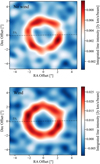 |
Fig. G.1 Moment-0 images for the no wind (top) and wind (bottom) cases. They look very similar given the low spatial resolution and sensitivity level and we need to look at the velocity component of the gas to clearly see the difference between the wind and Keplerian models. |
Appendix H Gas sample used
In Table H.1, we list the references from which we obtained the value of nd and ΔR we use to plot Figure 4. The sample includes both high-gas-density systems and low-density ones. It is not complete by any means but serves to guide our eyes on the different plots. The first column gives the star's name of the system with gas detected. The second column provides the method to calculate the gas density (gas mass, gas surface density) or “reference” if it is already provided as such in the reference. The third column is for the gas density that is either calculated from the mass, when provided, or directly taken from the papers listed in the Ref. column. The fourth column is for the belt's width AR and the last column provides the references we used to get both the gas amount and its width. We note that if there are two references, the first one if for the estimation of the amount of gas and the other for AR. We take the literature values as is and do not try to remodel everything homogeneously, which means that horizontal (width) as well as vertical (density) error bars may be quite large because sometimes the CO is not well resolved and/or the excitation or optical depth conditions are not very well known. Our plot rather shows the trend and that some disks may be in the WIND regime but dedicated studies should be carried out for each system to find out for sure.
References
- Axford, W. I., Dessler, A. J., & Gottlieb, B. 1963, ApJ, 137, 1268 [NASA ADS] [CrossRef] [Google Scholar]
- Balbus, S. A., & Hawley, J. F., 1991, ApJ, 376, 214 [Google Scholar]
- Beust, H., Lagrange-Henri, A. M., Vidal-Madjar A., & Ferlet, R., 1989, A&A, 223, 304 [NASA ADS] [Google Scholar]
- Beust, H., & Valiron, P., 2007, A&A, 466, 201 [NASA ADS] [CrossRef] [EDP Sciences] [Google Scholar]
- Biver, N., Bockelée-Morvan, D., Colom, P., et al., 2002, EM&P, 90, 5 [NASA ADS] [Google Scholar]
- Bockelée-Morvan, D., Crovisier, J., Mumma, M. J., & Weaver, H. A., 2004, Comets II, 391 [Google Scholar]
- Bockelée-Morvan, D., & Biver, N., 2017, RSPTA, 375, 20160252 [Google Scholar]
- Bouvier, J., 2013, EAS, 62, 143 [NASA ADS] [CrossRef] [EDP Sciences] [Google Scholar]
- Brandeker, A., Liseau, R., Olofsson, G., & Fridlund, M., 2004, A&A, 413, 681 [NASA ADS] [CrossRef] [EDP Sciences] [Google Scholar]
- Brown, G.N., & Ziegler, W. T., 1979, J. Chem. Eng. Data, 24, 319 [CrossRef] [Google Scholar]
- Castelli, F., & Kurucz, R. L., 2003, IAU Symp., 210, A20 [Google Scholar]
- Cataldi, G., Brandeker, A., Wu, Y., et al., 2018, ApJ, 861, 72 [NASA ADS] [CrossRef] [Google Scholar]
- Chen, C. H., & Jura, M., 2003, ApJ, 582, 443 [NASA ADS] [CrossRef] [Google Scholar]
- Chiang, E., & Fung, J., 2017, ApJ, 848, 4 [NASA ADS] [CrossRef] [Google Scholar]
- Cochran, A. L., & McKay, A. J., 2018, ApJ, 854, L10 [Google Scholar]
- Cordiner, M. A., Milam, S. N., Biver, N., et al., 2020, Nat. Astron., 4, 861 [Google Scholar]
- Cranmer, S. R., & van Ballegooijen, A. A., 2010, ApJ, 720, 824 [NASA ADS] [CrossRef] [Google Scholar]
- Cranmer, S. R., & Saar, S. H., 2011, ApJ, 741, 54 [Google Scholar]
- Davis, M. W., Gladstone, G. R., Greathouse, T. K., et al., 2011, SPIE, 8146, 814604 [NASA ADS] [Google Scholar]
- Dello Russo, N., Kawakita, H., Vervack, R. J., & Weaver, H. A., 2016, Icarus, 278, 301 [NASA ADS] [CrossRef] [Google Scholar]
- Dent, W. R. F., Wyatt, M. C., Roberge, A., et al., 2014, Science, 343, 1490 [NASA ADS] [CrossRef] [Google Scholar]
- Dhilip, K. T. J., Saieswari, A., & Kumar, S., 2006, J. Chem. Phys., 124, 034314 [NASA ADS] [CrossRef] [Google Scholar]
- Dialynas, K., Krimigis, S. M., Mitchell, D. G., Decker, R. B., & Roelof, E. C., 2017, Nat. Astron., 1, 0115 [NASA ADS] [CrossRef] [Google Scholar]
- Dullemond, C. P., Juhasz, A., Pohl, A., et al., 2012, Astrophysics Source Code Library [record ascl:1202.015] [Google Scholar]
- Duncan, M., Levison, H., & Dones, L., 2004, in Comets II, eds. M. C. Festou, H. U. Keller, & H. A. Weaver, 193 [Google Scholar]
- Fernández, Y. R., Kelley, M. S., Lamy, P. L., et al., 2013, Icarus, 226, 1138 [Google Scholar]
- Fernández, R., Brandeker, A., & Wu, Y., 2006, ApJ, 643, 509 [CrossRef] [Google Scholar]
- Ferrari, C., & Lucas, A., 2016, A&A, 588, A133 [NASA ADS] [CrossRef] [EDP Sciences] [Google Scholar]
- Gladstone, G. R., Stern, S. A., Ennico, K., et al., 2016, Science, 351, 8866 [NASA ADS] [CrossRef] [Google Scholar]
- Gladstone, G. R., Kammer, J. A., Adams, D. J., et al., 2021, Icarus, 356, 113973 [CrossRef] [Google Scholar]
- Goldsmith, P. F., & Langer, W. D., 1999, ApJ, 517, 209 [Google Scholar]
- Gomes, R., Levison, H. F., Tsiganis, K., & Morbidelli, A., 2005, Nature, 435, 466 [Google Scholar]
- Greathouse, T. K., Gladstone, G. R., Davis, M. W., et al., 2013, SPIE, 8859, 88590T [NASA ADS] [Google Scholar]
- Groussin, O., Attree, N., Brouet, Y., et al., 2019, Space Sci. Rev., 215, 29 [Google Scholar]
- Gueymard, C. A., 2018, Sol. Energy, 169, 434 [NASA ADS] [CrossRef] [Google Scholar]
- Guilbert-Lepoutre, A., 2012, AJ, 144, 97 [Google Scholar]
- Hartigan, P., Edwards, S., & Ghandour, L., 1995, ApJ, 452, 736 [Google Scholar]
- Heays, A. N., Bosman, A. D., & van Dishoeck, E. F., 2017, A&A, 602, A105 [NASA ADS] [CrossRef] [EDP Sciences] [Google Scholar]
- Higuchi, A. E., Kóspál, Á., Moór A., Nomura, H., & Yamamoto, S., 2020, ApJ, 905, 122 [NASA ADS] [CrossRef] [Google Scholar]
- Horányi, M., Hoxie, V., James, D., et al., 2008, Space Sci. Rev., 140, 387 [Google Scholar]
- Hosteaux, S., Chané, E., & Poedts, S., 2019, A&A, 632, A89 [NASA ADS] [CrossRef] [EDP Sciences] [Google Scholar]
- Hu, X., Gundlach, B., von Borstel, I., Blum, J., & Shi, X., 2019, A&A, 630, A5 [NASA ADS] [CrossRef] [EDP Sciences] [Google Scholar]
- Huebner, W. F., & Mukherjee, J., 2015, P&SS, 106, 11 [NASA ADS] [CrossRef] [Google Scholar]
- Huebner, W. F., Keady, J. J., & Lyon, S. P., 1992, Ap&SS, 195, 1 [NASA ADS] [CrossRef] [Google Scholar]
- Huebner, W. F., Benkhoff, J., Capria, M.-T., et al. 2006, in Heat and Gas Diffusion in Comet Nuclei [Google Scholar]
- Hughes, A. M., Lieman-Sifry, J., Flaherty, K. M., et al., 2017, ApJ, 839, 86 [NASA ADS] [CrossRef] [Google Scholar]
- Izmodenov, V., Malama, Y. G., & Lallement, R., 1997, A&A, 317, 193 [NASA ADS] [Google Scholar]
- Izmodenov, V. V., Lallement, R., & Geiss, J., 1999, A&A, 344, 317 [NASA ADS] [Google Scholar]
- Jewitt, D., Garland, C. A., & Aussel, H., 2008, AJ, 135, 400 [NASA ADS] [CrossRef] [Google Scholar]
- Jewitt, D., Kim, Y., Mutchler, M., Agarwal, J., Li, J., & Weaver, H., 2021, AJ, 161, 188 [NASA ADS] [CrossRef] [Google Scholar]
- Johnstone, C. P., Güdel, M., Lüftinger, T., Toth, G., & Brott, I., 2015, A&A, 577, A27 [NASA ADS] [CrossRef] [EDP Sciences] [Google Scholar]
- Johnstone, C. P., Güdel, M., Brott, I., & Lüftinger, T., 2015, A&A, 577, A28 [NASA ADS] [CrossRef] [EDP Sciences] [Google Scholar]
- Kiefer, F., Lecavelier, des Etangs, A., Boissier, J., et al., 2014, Nature, 514, 462 [NASA ADS] [CrossRef] [Google Scholar]
- Kim, M., Wolf, S., Löhne, T., Kirchschlager, F., & Krivov, A. V., 2018, A&A, 618, A38 [NASA ADS] [CrossRef] [EDP Sciences] [Google Scholar]
- Kóspál, Á., Moór, A., Juhász, A., et al., 2013, ApJ, 776, 77 [Google Scholar]
- Kral, Q., & Latter, H., 2016, MNRAS, 461, 1614 [NASA ADS] [CrossRef] [Google Scholar]
- Kral, Q., Wyatt, M., Carswell, R. F., et al. 2016, MNRAS, 461, 845 [NASA ADS] [CrossRef] [Google Scholar]
- Kral, Q., Matrà, L., Wyatt, M. C., & Kennedy, G. M. 2017, MNRAS, 469, 521 [NASA ADS] [CrossRef] [Google Scholar]
- Kral, Q., Marino, S., Wyatt, M. C., 2019, MNRAS, 489, 3670 [NASA ADS] [Google Scholar]
- Kral, Q., Davoult, J., & Charnay, B., 2020a, Nat. Astron., 4, 769 [Google Scholar]
- Kral, Q., Matrà, L., Kennedy, G. M., Marino, S., & Wyatt, M. C., 2020b, MNRAS, 497, 2811 [NASA ADS] [CrossRef] [Google Scholar]
- Kral, Q., Pringle, J. E., Guilbert-Lepoutre, A., et al., 2021, A&A, 653, L11 [NASA ADS] [CrossRef] [EDP Sciences] [Google Scholar]
- Krijt, S., Schwarz, K. R., Bergin, E. A., & Ciesla, F. J., 2018, ApJ, 864, 78 [Google Scholar]
- Krivov, A. V., & Wyatt, M. C., 2021, MNRAS, 500, 718 [Google Scholar]
- Krtivcka, J., 2014, A&A, 564, A70 [NASA ADS] [CrossRef] [EDP Sciences] [Google Scholar]
- Lanz, T., & Catala, C., 1992, A&A, 257, 663 [NASA ADS] [Google Scholar]
- Lisse, C. M., Young, L. A., Cruikshank, D. P., et al., 2021, Icarus, 356, 114072 [CrossRef] [Google Scholar]
- López-Patiño, J., Fuentes, B. E., Yousif, F. B., & Martínez, H., 2017, Phys. Procedia,, 90, 391 [CrossRef] [Google Scholar]
- Lovell, J. B., Kennedy, G. M., Marino, S., et al., 2021, MNRAS, 502, L66 [NASA ADS] [CrossRef] [Google Scholar]
- Luhman, K. L., 2020, AJ, 160, 186 [NASA ADS] [CrossRef] [Google Scholar]
- Luu, J. X., & Jewitt, D. C., 2002, ARA&A, 40, 63 [NASA ADS] [CrossRef] [Google Scholar]
- MacGregor, M. A., Matrà, L., Kalas, P., et al., 2017, ApJ, 842, 8 [CrossRef] [Google Scholar]
- Marino, S., Matrà, L., Stark, C., et al., 2016, MNRAS, 460, 2933 [Google Scholar]
- Marino, S., Wyatt, M. C., Panic, O., et al., 2017, MNRAS, 465, 2595 [NASA ADS] [CrossRef] [Google Scholar]
- Marino, S., Flock, M., Henning, T., Kral, Q., Matrà, L., & Wyatt, M. C., 2020, MNRAS, 492, 4409 [NASA ADS] [CrossRef] [Google Scholar]
- Masuoka, T., & Samson, J. A. R., 1980, J. Chem. Phys., 77, 623 [NASA ADS] [Google Scholar]
- Matrà, L., Panic, O., Wyatt, M. C., & Dent, W. R. F., 2015, MNRAS, 447, 3936 [CrossRef] [Google Scholar]
- Matrà, L., Dent, W. R. F., Wyatt, M. C., et al., 2017a, MNRAS, 464, 1415 [Google Scholar]
- Matrà, L., MacGregor, M. A., Kalas, P., et al., 2017b, ApJ, 842, 9 [Google Scholar]
- Matrà, L., Wilner, D. J., Öberg, K. I., et al. 2018a, ApJ, 853, 147 [Google Scholar]
- Matrà, L., Marino, S., Kennedy, G. M., Wyatt, M. C., Öberg, K. I., & Wilner, D. J., 2018b, ApJ, 859, 72 [CrossRef] [Google Scholar]
- Matrà, L., Öberg, K. I., Wilner, D. J., Olofsson, J., & Bayo, A., 2019, AJ, 157, 117 [Google Scholar]
- McMullin, J. P., Waters, B., Schiebel, D., Young, W., & Golap, K., 2007, ASP Conf. Ser., 376, 127 [Google Scholar]
- Meier, R. R., 1991, Space Sci. Rev., 58, 1 [NASA ADS] [CrossRef] [Google Scholar]
- Meyer-Vernet, N., Issautier, K., 1998, J. Geophys. Res., 103, 29705 [NASA ADS] [CrossRef] [Google Scholar]
- Miller, T. M., & Bederson, B., 1978, Adv. Atm. Mol. Phys., 13, 1 [NASA ADS] [CrossRef] [Google Scholar]
- Moór, A., Juhász, A., Kóspál, Á., et al., 2013, ApJ, 777, L25 [CrossRef] [Google Scholar]
- Moór, A., Curé, M., Kóspál, Á., et al., 2017, ApJ, 849, 123 [Google Scholar]
- Moór, A., Kral, Q., Ábrahám, P., et al., 2019, ApJ, 884, 108 [CrossRef] [Google Scholar]
- Morbidelli, A., Nesvorny, D., Bottke, W. F., & Marchi, S., 2021, Icarus, 356, 114256 [CrossRef] [Google Scholar]
- Nahar S. N., 1999, ApJS, 120, 131 [NASA ADS] [CrossRef] [Google Scholar]
- Nahar, S. N., & Pradhan, A. K., 1997, ApJS, 111, 339 [NASA ADS] [CrossRef] [Google Scholar]
- Nesvorný, D., Vokrouhlický, D., Stern, A. S., et al., 2019, AJ, 158, 132 [Google Scholar]
- Niedner-Schatteburg, G., & Toennies, J. P., 1992, J. Chem. Phys., LXXXII, 553 [Google Scholar]
- Nilsson, R., Brandeker, A., Olofsson, G., et al. 2012, A&A, 544, A134 [NASA ADS] [CrossRef] [EDP Sciences] [Google Scholar]
- Nisini, B., Milillo, A., Saraceno, P., & Vitali, F., 1995, A&A, 302, 169 [NASA ADS] [Google Scholar]
- Olney, T. N., Cann, N. M., Cooper, G., & Brion, C. E., 1997, Chem. Phys., 223, 59 [NASA ADS] [CrossRef] [Google Scholar]
- Olofsson, J., van Holstein, R. G., Boccaletti, A., et al., 2018, A&A, 617, A109 [NASA ADS] [CrossRef] [EDP Sciences] [Google Scholar]
- Opher, M., Loeb, A., Drake, J., & Toth, G., 2020, Nat. Astron., 4, 675 [NASA ADS] [CrossRef] [Google Scholar]
- Planck Collaboration XIII. 2014, A&A, 571, A13 [NASA ADS] [CrossRef] [EDP Sciences] [Google Scholar]
- Plavchan, P., Werner, M. W., Chen, C. H., et al. 2009, ApJ, 698, 1068 [Google Scholar]
- Poppe, A. R., Lisse, C. M., Piquette, M., et al., 2019, ApJ, 881, L12 [NASA ADS] [CrossRef] [Google Scholar]
- Prialnik, D., Benkhoff, J., & Podolak, M., 2004, in Comets II, eds. M. C. Festou, H. U. Keller, & H. A. Weaver, 359 [Google Scholar]
- Rebollido, I., Eiroa, C., Montesinos, B., et al., 2018, A&A, 614, A3 [NASA ADS] [CrossRef] [EDP Sciences] [Google Scholar]
- Rebollido, I., Ribas, Á., de Gregorio-Monsalvo, I., et al., 2022, MNRAS, 509, 693 [Google Scholar]
- Richardson, J. D., Belcher, J. W., Garcia-Galindo, P., Burlaga, L. F., 2019, Nat. Astron., 3, 1019 [NASA ADS] [CrossRef] [Google Scholar]
- Roberge, A., Feldman, P. D., Lagrange, A. M., et al., 2000, ApJ, 538, 904 [NASA ADS] [CrossRef] [Google Scholar]
- Rubin, M., Hansen, K. C., Gombosi, T. I., et al. 2009, Icarus, 199, 505 [NASA ADS] [CrossRef] [Google Scholar]
- Sezestre, É., Augereau, J.-C., Boccaletti, A., & Thébault, P., 2017, A&A, 607, A65 [NASA ADS] [CrossRef] [EDP Sciences] [Google Scholar]
- Shakura, N. I., & Sunyaev, R. A., 1973, A&A, 24, 337 [NASA ADS] [Google Scholar]
- Sibthorpe, B., Kennedy, G. M., Wyatt, M. C., et al. 2018, MNRAS, 475, 3046 [Google Scholar]
- Smirnov-Pinchukov, G. V., Moór, A., Semenov, D. A., et al., 2021, MNRAS, 510, 1148 [NASA ADS] [CrossRef] [Google Scholar]
- Stern, S. A., Slater, D. C., Scherrer, J., et al., 2008, Space Sci. Rev., 140, 155 [NASA ADS] [CrossRef] [Google Scholar]
- Teague, R., & Foreman-Mackey, D., 2018, RNAAS, 2, 173 [NASA ADS] [Google Scholar]
- Thébault, P., 2009, A&A, 505, 1269 [Google Scholar]
- Tiscareno, M. S., & Malhotra, R., 2003, AJ, 126, 3122 [NASA ADS] [CrossRef] [Google Scholar]
- Visser, R., van Dishoeck, E. F., & Black, J. H., 2009, A&A, 503, 323 [NASA ADS] [CrossRef] [EDP Sciences] [Google Scholar]
- Vitense, C., Krivov, A. V., Kobayashi, H., & Löhne, T., 2012, A&A, 540, A30 [NASA ADS] [CrossRef] [EDP Sciences] [Google Scholar]
- Wakelam, V., Herbst, E., Loison, J.-C., et al., 2012, ApJS, 199, 21 [Google Scholar]
- Wierzchos, K., Womack, M., & Sarid, G., 2017, AJ, 153, 230 [NASA ADS] [CrossRef] [Google Scholar]
- Womack, M., Sarid, G., Wierzchos, K., 2017, PASP, 129, 031001 [NASA ADS] [CrossRef] [Google Scholar]
- Wyatt, M. C., 2005, A&A, 433, 1007 [NASA ADS] [CrossRef] [EDP Sciences] [Google Scholar]
- Wyatt, M. C., Smith, R., Su, K. Y. L., et al. 2007, ApJ, 663, 365 [NASA ADS] [CrossRef] [Google Scholar]
- Wyatt, M. C., Clarke, C. J., & Booth, M., 2011, Celest. Mech. Dyn. Astron., 111, 1 [NASA ADS] [CrossRef] [Google Scholar]
- Youngblood, A., Roberge, A., MacGregor, M. A., et al., 2021, AJ, 162, 235 [NASA ADS] [CrossRef] [Google Scholar]
We note that thit is not linked to the mean-free path of protons, λw, through the disk but rather to the mean-free path of a gas particle experiencing a flux of incoming protons, as described in Appendix B.
Given the uncertainties on the age of the system, NO Lup could also be amain sequence star of 12–15 Myr (member of UCL, Luhman 2020).
All Tables
All Figures
|
Fig. 1 Cartoon showing the different dynamics of the gas as a function of gas density and stellar luminosity. The critical density and luminosity showed on the figure are approximate and more precise values are presented in the paper. This paper focuses on the Stellar wind mechanism, circled in red. |
| In the text | |
|
Fig. 2 Steady-state gas density in the belt (in Keplerian motion) as predicted by our model for different values of gas production rate. The line in red represents ncrit which is the critical density below which the gas has a wind structure (see Eq. (5)) for collisions between SW protons and either C, O, or ions. Above this critical density, the gas is assumed to form a viscous disk with α = 10−3. The case of high Msw = 105 Ṁ⊙ shows the regime where tleave/thit > 1, independent of Ṁsw where we assume υsw = 100 km/s (see main text for details). |
| In the text | |
|
Fig. 3 Ratio of density between gas in the wind (spherical outward motion) to that in the belt (in Keplerian motion in the belt), at the belt location, R, as a function of the stellar wind mass-loss rate. For this plot, we use Eq. (10) with µ = 28, υsw = 100 km/s, R = 100 au, ΔR = 50 au, σcol = 2 × 10⁻¹⁸ m2, and H = 0.05R. For a stellar wind mass-loss rate that is a few tens of that of the Sun, values of nw become greater than nd and the wind becomes dominant. |
| In the text | |
|
Fig. 4 Critical density ncrit vs. the belt width ΔR. Lines represent the critical density ncrit at which the gas transition from a disk to a wind vs. ΔR. The solid line is for a model where ncrit is given by Eq. (5) and assumes that protons collide with ions, C or O. The dashed line is for collisions between protons and CO. We indicate in capital letters whether the gas would be more DISK- or WIND-like in different regions of the plot. We note that under the black lines, winds are very likely to behave as stated in the main text. The blue points show the gas density nd estimated for the different systems shown in the plot. A vertical line joins two blue dots when a range of values are given in the literature for the gas densities or masses. Data are given in Table H.1. |
| In the text | |
|
Fig. 5 Simulated spectra of the J = 3−2 CO line for TWA 7 for the no wind case (solid), and wind (dash-dotted) cases. Along with the moment-0 image of the disk, one can identify that the wind profile is not Keplerian but it is even more clearly visible on the moment-1 images in Fig. 7 (because the velocity structure changes significantly). |
| In the text | |
|
Fig. 6 Wind structure for a belt extending from 60 to 90 au. Top: wind density in a (X, Y) plane at Z = 0 (cut in the midplane). The density was set to 1 cm−3 for the wind emerging from the belt. Middle: wind density in a (X, Z) plane at Y = 0 (cut at the middle of the belt). Bottom: velocity structure (direction and magnitude) integrated along the line of sight (assumed here to be along the Y axis). The red hatches show the location of the belt that releases gas. |
| In the text | |
|
Fig. 7 Moment-1 images (intensity-weighted velocity) for the no wind (top) and wind (bottom) cases. The no-wind Keplerian case is aligned on the disk position angle while it is very inclined or even perpendicular for the wind case, making them easily distinguishable, which can also be seen on the position-velocity diagram (Fig. 8). |
| In the text | |
|
Fig. 8 Position-velocity (PV) diagrams for the no wind (top) and wind (bottom) cases. The no-wind Keplerian case shows a typical PV diagram for a Keplerian disk along its position angle while it is horizontal for the wind case, making them easily distinguishable. |
| In the text | |
|
Fig. 9 Transition between disk and wind regions shown in the space of the fractional luminosity of a debris disk as a function of the host star luminosity. The bottom left and far right regions are likely to be populated by gas having a wind structure while the upper left region would more likely be filled by circumstellar gas disks. We show the limit between disk and wind cases for two values of α: 0.1 (solid) and 0.01 (dashed). The thin red and blue lines are dust detection limits of ALMA at 870 microns and Herschel at 70 microns assuming dust lies at 100 au. See the assumptions behind this plot at the end of Appendix C. |
| In the text | |
|
Fig. B.1 Steady-state gas density in the belt predicted by our model as a function of r, which is the radial distance to the star. The fiducial model has a = 1, b = 0, R0 = 100 au, h0 = 0.05, ṀSW = 1.4 × 10⁻¹⁴ M⊙/yr, and Ṁg = 10−3 M⊕/Myr (see Eq. B.7). Values below Rcrit (see Eq. B.8), i.e., above the red line, are not shown. The density beyond the planetesimal width ΔR will mostly scale as r−2 as the fiducial model (see Appendix G) but it is not represented in the plot. |
| In the text | |
|
Fig. D.1 Schematic of the collision between a proton of initial velocity υp with a gas particle. The collision angle ψ is between the normal to the surfaces of the spheres at the point of contact and the proton velocity. |
| In the text | |
|
Fig. E.1 Timescales for ionization tion (red), leaving the disk tleave (orange), and stellar wind collisions with CO thit (blue) Vs distance to the gas. The fiducial model labeled as the “young system” has M⋆ = 1M⊙, υsw = 100 km/s, and Ω⋆ = 10 Ω⋆. The timescale tion for SW protons is shown for a young system but it is always an order of magnitude greater than thit. |
| In the text | |
|
Fig. G.1 Moment-0 images for the no wind (top) and wind (bottom) cases. They look very similar given the low spatial resolution and sensitivity level and we need to look at the velocity component of the gas to clearly see the difference between the wind and Keplerian models. |
| In the text | |
Current usage metrics show cumulative count of Article Views (full-text article views including HTML views, PDF and ePub downloads, according to the available data) and Abstracts Views on Vision4Press platform.
Data correspond to usage on the plateform after 2015. The current usage metrics is available 48-96 hours after online publication and is updated daily on week days.
Initial download of the metrics may take a while.