© The Authors 2024

1 Introduction

Debris disks are an integral component of (exo)planetary systems and are recognized as good record holders of important insights about their origins and dynamical histories (e.g., Wyatt 2008; Hughes et al. 2018). They emerge after most of the gas in protoplanetary disks is gone, that is, when systems are older than a few million years (typically 10–100 Myr). These disks are viewed as massive or younger counterparts of the asteroid belt and the Kuiper belt in the present-day Solar System.

Debris disks are, by definition, gas free or at least gas poor, and hence detections of gas in the disks have been a fundamental mystery (Slettebak 1975; Hobbs et al. 1985)¹. The importance of this problem has recently been boosted by unexpected detections of CO gas in ∼20 relatively young (∼10–100 Myr) debris disks (e.g., Dent et al. 2014; Moór et al. 2017; Kral et al. 2017; Marino et al. 2020; Rebollido et al. 2022). Successful detections of gas in debris disks are still very limited, as high-sensitivity observations with long integration times are required, even for known massive debris disks. The advent of Herschel and Atacama Large Millimeter Array (ALMA) made it possible to conduct such observations, which detect the absorption and emission lines originating from atomic and molecular gas in debris disks, including C, O, Na, Mg, Ca, Mn, Fe, Ni, Ti, Cr (e.g., Hobbs et al. 1985; Brandeker et al. 2004), and CO (e.g., Dent et al. 2014; Hughes et al. 2017). For emission lines, CO gas is the only confirmed molecule so far. Ongoing JWST observations aim to discover other molecules, including hot water vapor.

Two competing hypotheses for understanding the origin of gas in debris disks are currently proposed (Fig. 1, e.g., Kral et al. 2016; Marino et al. 2020; Nakatani et al. 2021; Smirnov-Pinchukov et al. 2022). The first is that observed gas may be left over from massive gaseous protoplanetary disks, that is, it may be of primordial origin, and the competing one is that the gas may have been generated recently by planetesimals colliding after gas disks dissipate, that is, it may be of secondary origin². We refer to these two hypotheses as Hypothesis 1 and Hypothesis 2, respectively. A current outstanding issue is that observations of CO gas alone cannot reliably determine which hypothesis is dominant.

We propose here that water vapor can serve as a better probe for differentiating the origin of gas in debris disks. By performing order-of-magnitude calculations and comparing them with existing observations, we show that the mass of cold water vapor as a function of CO mass exhibits a non-monotonic distribution, leading to better differentiation. The detection of such water vapor will become possible only with a future far-IR (FIR) space observatory. This work therefore supports the case for development of an FIR space probe mission to reveal the origin of gas in debris disks and the evolution of planet-forming disks in general.

Fig. 1 Schematic diagram of time evolution of planet-forming disks. The host star is denoted by the star symbol, planet-forming materials are represented by the brown and blue dots, and disk gas by the green ovals. Hypothesis 1 considers that observed gas is the leftover of primordial gas, while Hypothesis 2 considers that the gas is produced by collisions among icy bodies.

2 Determining the origin of gas

2.1 Basic picture

We begin by introducing a basic picture of the problem. The origin of gas in debris disks may be explained by two hypotheses that correspond to two distinct environments achieved during disk evolution (Fig. 1): Hypothesis 1 focuses on the end stage of protoplanetary disks, where primordial disk gas is still present, and Hypothesis 2 targets debris disks, where there is no primordial gas, and if gas is present, itis produced by collisions between icy bodies.

In the protoplanetary disk-like environment, the presence of CO gas (and dust) is confirmed by detections of their emission; most of the CO is in the gas phase when the temperature is higher than its freeze-out temperature of ~20 K. This indicates that the abundance of observed CO gas is regulated predominantly by gas-phase chemistry. On the other hand, there is no primordial gas in a gas-poor environment such as a debris disk. Therefore, gas is produced by collisions among icy bodies³ . This suggests that the abundance of observed CO gas is controlled by physical and chemical processes operating in the solid phase; freeze-out of released CO gas is negligible due to its freeze-out temperature being lower than that of the surrounding environment. Thus, the difficulty of constraining the origin of gas in debris disks using CO gas alone is attributed to the underlying conditions (i.e., gas vs. solid phases) considered in the two hypotheses.

Here, we propose to focus on cold water vapor. In the protoplanetary disk-like environment, hot (or warm) and cold water vapor are present; the former has temperatures of ~200–1500 K⁴, and the latter temperatures of ≲100 K. We currently consider outer parts of disks, where observed CO gas and solids reside, and hence it is reasonable to focus on cold water vapor. The temperature of cold water vapor is well below the freeze-out temperature of water, and hence its origin is attributed to photodesorption from dust grains due to attenuated interstellar UV radiation (Willacy & Langer 2000; Dominik et al. 2005). The presence of cold water vapor has already been confirmed by observations of protoplanetary disks (e.g., Hogerheijde et al. 2011). Any detection of water vapor in debris disks is not yet claimed in the literature. If present, it should be classified as cold water vapor due to the location of debris disks in relation to the host star; water vapor produced by collisions between icy bodies remains in the gas phase because photodesorption prevents complete freeze-out⁵.

In summary, focusing on cold water vapor enables us to unify the fundamental process operating in the two hypotheses, and hence the origin of gas in debris disks is better constrained. In the following, we demonstrate this using order-of-magnitude analyses.

2.2 Order-of-magnitude analysis

First, it is useful to estimate when the protoplanetary disk stage ends and the debris disk stage starts. Such a transition occurs when photoevaporation plays the dominant role in the dispersal of primordial disk gas (e.g., Hollenbach et al. 1994; Clarke et al. 2001; Alexander et al. 2014).

Given that a typical photoevaporation rate is ~10^–10M_⊙ yr^–1 and the transition phase may last for ~10⁵ yr (e.g., Alexander et al. 2014)⁶, a typical value for the gas mass at the transition (M_gas,tran) is given as M_gas,tran ~ 10^–10M_⊙ yr^–1 × 10⁵ yr ~ 1M_⊕. A characteristic value of observed CO gas mass at the transition (${\overline{M}}_{\text{CO},\text{ tran }}$) is then written as $${\overline{M}}_{\text{CO, tran }}\simeq f_{\text{CO, gas }}{M}_{\text{gas,tran }}~{10}^{-3}{M}_{\oplus },$$(1)

where $$\begin{array}{l}{f}_{\text{CO,gas}}\equiv \frac{M_{\text{CO,gas}}}{M_{\text{gas}}}\simeq \frac{M_{\text{CO,gas}}}{M_{{\text{H}}_2}}=\frac{m_{\text{CO}}{N}_{\text{CO}}}{m_{{\text{H}}_2}{N}_{{\text{H}}_2}}~{10}^{-3}\\ ~\frac{{\overline{M}}_{\text{CO, tran }}}{M_{\text{gas,tran}}};\end{array}$$(2)

M_gas, $M_{{\text{H}}_2}$, and M_CO,gas are the total, molecular hydrogen, and CO gas masses, respectively, and $N_{\text{CO}}/N_{{\text{H}}_2}\simeq {10}^{-4}$ is a typical value inferred for the interstellar medium (ISM, e.g., Bolatto et al. 2013). Interestingly, this simple estimate is broadly consistent with a detailed estimate derived from disk observations (Cataldi et al. 2023).

We computed the mass ratio of CO gas to dust (M_solid) for both hypotheses to examine how CO gas may be used to differentiate these hypotheses. For Hypothesis 1, the mass ratio can be written as $${\frac{{\overline{M}}_{\text{CO}}}{{\overline{M}}_{\text{solid }}}|}_{\text{Hyp}1}\simeq \frac{M_{\text{CO},\text{ gas }}}{M_{\text{solid }}}=\frac{M_{\text{CO},\text{ gas }}}{M_{\text{gas }}}\frac{M_{\text{gas }}}{M_{\text{solid }}}\simeq f_{\text{CO},\text{ gas }}{f}_{\text{GtoS}},$$(3)

where ${\overline{M}}_{\text{CO}}$ and ${\overline{M}}_{\text{solid}}$ are the observed CO gas and dust masses, respectively, and the mass ratio of gas to solids is often called the gas-to-solid (or gas-to-dust) ratio: $$f_{\text{GtoS}}\equiv \frac{M_{\text{gas}}}{M_{\text{solid }}}~{10}^2,$$(4)

where the typical value (i.e., f_GtoS ~ 10²) widely used for the initial stage of protoplanetary disks is adopted. Consequently, $${\frac{{\overline{M}}_{\text{CO}}}{{\overline{M}}_{\text{solid}}}|}_{\text{Hyp}1}\simeq {10}^{-1}\left(\frac{f_{\text{CO},\text{gas}}}{{10}^{-3}}\right)\left(\frac{f_{\text{GtoS}}}{{10}^2}\right).$$(5)

Our calculations thus suggest that Hypothesis 1 predicts that ${\overline{M}}_{\text{CO}}/{\overline{M}}_{\text{solid }}~0.1$ in the protoplanetary disk-like environment. Possible variations of ${\overline{M}}_{\text{CO}}/{\overline{M}}_{\text{solid }}$ are discussed in the next section. It should be noted that, in protoplanetary disks, solids may be in the form of dust as well as in the form of much larger bodies such as planetesimals and (proto)planets. Accordingly, our assumption (i.e., ${\overline{M}}_{\text{solid }}\simeq M_{\text{solid }}$) in Eq. (3) leads to an upper limit for the observed mass ratio.

For Hypothesis 2, we may assume that on average the observed mass ratio of CO to solids reflects the bulk composition of icy bodies, since collisions among various bodies would occur. Such colliding bodies may have a mass ratio of ice to refractory materials, also known as the ice-to-rock ratio, of $$f_{\text{ItoR}}\equiv \frac{M_{Z,\text{ice}}}{M_{Z,\text{ref}}}~0.1,$$(6)

where a characteristic value of f_ItoR(~ 10^–1) inferred from comets and Kuiper belt objects is adopted (e.g., Biver et al. 2019; Fulle et al. 2019; Combi et al. 2020; Marschall et al. 2020; Choukroun et al. 2020; Davidsson et al. 2022). Then ${\overline{M}}_{\text{CO}}/{{\overline{M}}_{\text{solid}}|}_{\text{Hyp}2}$ is written as $${\frac{{\overline{M}}_{\text{CO}}}{{\overline{M}}_{\text{solid }}}|}_{\text{Hyp}2}\simeq \frac{M_{\text{CO},\text{ ice }}}{M_{Z,\text{ ref }}}=\frac{M_{\text{CO},\text{ ice }}}{M_{Z,\text{ ice }}}\frac{M_{Z,\text{ ice }}}{M_{Z,\text{ ref }}}\simeq f_{\text{CO},\text{ ice }}{f}_{\text{ItoR}},$$(7)

where $$f_{\text{CO},\text{ ice }}\equiv \frac{M_{\text{CO},\text{ ice }}}{M_{\text{Z},\text{ ice }}}\simeq \frac{M_{\text{CO},\text{ ice }}}{M_{{\text{H}}_2\text{O},\text{ ice }}}\simeq \frac{m_{\text{CO}}{N}_{\text{CO},\text{ ice }}}{m_{{\text{H}}_2\text{O}}{N}_{{\text{H}}_2\text{O},\text{ ice }}}~{10}^{-1},$$(8)

where it is assumed that $M_{Z,\text{ ice }}\simeq M_{{\text{H}}_2\text{O},\text{ ice }}$, which is reasonable for comets observed in the Solar System, and a characteristic value of $N_{\text{CO},\text{ice}}/N_{{\text{H}}_2\text{O},\text{ice }}\left(\simeq {10}^{-1}\right)$ inferred for them is used (e.g., Mumma & Charnley 2011; Harrington Pinto et al. 2022)⁷.

Consequently, $${\frac{{\overline{M}}_{\text{CO}}}{{\overline{M}}_{\text{solid }}}|}_{\text{Hyp}2}\simeq {10}^{-2}\left(\frac{f_{\text{CO},\text{ ice }}}{{10}^{-1}}\right)\left(\frac{f_{\text{ItoR}}}{{10}^{-1}}\right).$$(9)

We emphasize that this is a very simple estimate derived from the order-of-magnitude analysis. In reality, different bodies have different sizes and compositions, resulting in different production rates of CO gas. Also, care is needed because the values used in Eq. (9) come mainly from coma gas abundance ratios, which do not necessarily reflect nucleus ice abundance ratios.

Thus, our order-of-magnitude analysis indicates that the two hypotheses lead to different values of the CO-to-solid mass ratio, and the transition would occur at around M_CO ∼ 10^–3 M_⊕. It is, however, important to recognize that certain characteristic values are used to obtain the above theoretical estimates. These values may vary significantly for different targets.

2.3 Comparison with observations

Here, we examine how different disk properties would change the above theoretical estimates. By comparing these with existing observational data, we explore how reliable the CO-to-solid mass ratio is for differentiating the two hypotheses.

We first compared the theoretical estimates derived in the above section with observational data. Figure 2 depicts three estimates (${\overline{M}}_{\text{CO}}/{{\overline{M}}_{\text{solid }}|}_{\text{Hyp}1},{\overline{M}}_{\text{CO}}/{{\overline{M}}_{\text{solid }}|}_{\text{Hyp}2}$, and ${\overline{M}}_{\text{CO},\text{ tran }}$) with the solid red, dashed orange, and dotted black lines, respectively (see Eqs. (5), (9), and (1)). We adopted the observational data from Rebollido et al. (2022), in which the mass estimates of CO and dust were compiled for 21 targets, using their observations as well as collecting data from the literature (Moór et al. 2017, 2019; Di Folco et al. 2020). As expected, the comparison suggests that Hypothesis 1 works well for CO-gas-rich systems, while Hypothesis 2 can explain some CO-gas-poor systems. It is, however, clear that adopting certain characteristic values cannot reproduce all the observations.

We then explored the variation of disk parameters. Possible ranges of disk parameters (f_CO,gas, f_Gtos, f_co,ice, and f_itoR) were determined from previous studies (Table 1). It is immediately noticeable that disk parameters span a wide range of values, and as a result, both hypotheses cover large areas of Fig. 2; such areas are denoted by the shaded red and orange regions for Hypotheses 1 and 2, respectively.

The wide range of the CO-to-solid mass ratio indicates two points. The first is that, even if different targets have different disk properties, high CO masses tend to be explained well by Hypothesis 1 (i.e., observed gas is very likely of primordial origin), while low CO masses are better explained by Hypothesis 2 (i.e., the gas is likely produced by collisions among icy bodies). This thus suggests that order-of-magnitude analysis is useful for developing our basic understanding. The second point is, however, that both Hypotheses 1 and 2 can cover the same values of the CO-to-solid mass ratio (i.e., from 10^-4 to 0.1), and hence it is not straightforward to reliably differentiate the origin of observed gas. We can distinguish between Hypotheses 1 and 2 by specifying ${\overline{M}}_{\text{CO},\text{tran}}$ (Eq. (1)), yet the monotonic decrease in the CO-to-solid mass ratio with the CO mass makes the transition ambiguous. If another probe predicted non-monotonic distributions, more reliable determination would be possible.

Thus, our analysis shows that both hypotheses can reproduce existing observational data, and hence they are both viable. However, the resulting mass ratios indicate that the origin of gas in debris disks cannot be reliably determined from the value of ${\overline{M}}_{\text{CO}}/{\overline{M}}_{\text{solid }}$.

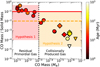Fig. 2 Mass ratio of CO gas to solids as a function of CO gas mass. The theoretical estimates derived from the order-of-magnitude analysis are denoted by the solid red, dashed orange, and dotted black lines, respectively (see Eqs. (5), (9), and (1)). For comparison, the observed data are included (Moór et al. 2017, 2019; Di Folco et al. 2020; Rebollido et al. 2022); the circles represent targets that exhibit detections of both CO gas and dust, the triangles are for targets with dust-only detections (i.e., the upper limit for CO gas mass), and the diamonds are for targets with upper limits for both CO gas and dust. The color of each data point corresponds to the age of the target, as shown in the color bar on the right. Different disk parameters lead to different values of the CO-tosolid mass ratio (Table 1). The shaded red and orange regions represent possible ranges corresponding to Hypotheses 1 and 2, respectively. It is clear that the CO-to-solid mass ratio is not a reliable probe for tightly constraining the origin of the observed gas.

2.4 The importance of water vapor

Here, we discuss how the degeneracy discussed above can be broken and the origin of observed gas can be better constrained. In this work, we propose to focus on water vapor, resulting in non-monotonic behavior of the mass ratio.

As discussed in Sect. 2.1, the presence of water vapor can be expected under both hypotheses and explained by photodesorption, which works as follows. At the disk surface, unattenuated UV radiation photodissociates water gas entirely, that is, no water vapor is present. On the other hand, UV radiation is completely attenuated at the disk midplane, and water gas freezes completely onto dust grains. In between, attenuated UV flux is too weak to photodissociate water gas entirely, but is still strong enough for photodesorption to prevent complete freeze-out of water molecules onto dust grains (Hollenbach et al. 2009). In such photodesorption-dominated regions, cold water vapor can be present.

The abundance of cold water vapor is then essentially insensitive to the UV flux (Dominik et al. 2005; Du & Bergin 2014). This is because the abundance is determined mainly by photodesorption and photodissociation, which are both controlled by the UV flux. Consequently, we computed the abundance of water vapor ($N_{{\text{H}}_2\text{O, vap }}$) as $${\sigma }_{\text{photo }}{N}_{{\text{H}}_2\text{O},\text{ vap }}={\sigma }_{\text{dust }}Y{N}_{\text{dust }},$$(10)

where σ_photo is the photodissociation cross section of water, ${\sigma }_{\text{dust }}=\pi r_{\text{dust }}^2$ is the cross-section of dust particles with a radius of r_dust, Y is the photodesorption yield of water, and N_dust is the abundance of dust particles contributing to photodesorption, which may differ for different hypotheses. In the following calculations, we adopted the standard values of Y (~10^–3, Westley et al. 1995; Öberg et al. 2009) and of σ_photo(= R₀/F₀ ~10^–17 cm²), where R₀ ~ 10^–9 s^–1 is the unshielded photodissociation rate of water at G₀ = 1⁸ (e.g., Hollenbach et al. 2009), and F₀ ~ 10⁸ photons cm^–2 s^–1 is the flux of UV photons at G₀ = 1.

It should be noted that the presence of CO gas is confirmed only for debris disks, where UV radiation from the host star is weak enough that interstellar UV radiation plays a major role in photodissociation (Kral et al. 2017). Hence, we focus on interstellar UV radiation in this work. We confirm that our abundance estimates do not change very much even if stellar UV radiation plays a dominant role (Appendix B).

Next, we computed the mass ratio of water vapor (${\overline{M}}_{{\text{H}}_2\text{O}}$) to CO gas. For Hypothesis 1, N_dust in Eq. (10) can be expressed as N_dust ≡ f_dustM_solid/m_dust, where f_dust is a factor taking account of the dust abundance relative to the total solid abundance, and $m_{\text{dust }}=4\pi {\rho }_{\text{dust }}{r}_{\text{dust }}^3/3$ is the mass of dust particles that have the bulk density of ρ_dust Then, we can write the ratio of $N_{{\text{H}}_2\text{O,vap }}$ to $N_{{\text{H}}_2}$ as $$\frac{N_{{\text{H}}_2\text{O,vap }}}{N_{{\text{H}}_2}}=Y\frac{{\sigma }_{\text{dust }}}{{\sigma }_{\text{photo }}}\frac{N_{\text{dust }}}{N_{{\text{H}}_2}}~{10}^{-9}{\left(\frac{f_{\text{GtoS}}}{{10}^2}\right)}^{-1}{\left(\frac{r_{\text{dust }}}{0.1\text{μ} \text{m}}\right)}^{-1},$$(11)

where it is assumed that dust particles with a characteristic size of r_dust(~0.1 µm) are most important for photodesorption. In order to better reproduce the result of Du & Bergin (2014, see their Eq. (29)) and the observation of cold water vapor in a pro- toplanetary disk (Hogerheijde et al. 2011), the abundance of such dust particles is set at 1% (i.e., f_dust = 10^–2), which reflects the effect of dust growth and settling.

Consequently, the ratio (${\overline{M}}_{{\text{H}}_2\text{O}}/{\overline{M}}_{\text{CO}}$) for Hypothesis 1 can be written as $$\begin{array}{l}{\frac{{\overline{M}}_{{\text{H}}_2\text{O}}}{{\overline{M}}_{\text{CO}}}|}_{\text{Hyp1}}\simeq \frac{m_{{\text{H}}_2\text{O}}{N}_{{\text{H}}_2\text{O, vap }}}{M_{\text{CO},\text{gas }}}=\frac{M_{{\text{H}}_2}}{M_{\text{CO},\text{gas}}}\frac{m_{{\text{H}}_2\text{O}}{N}_{{\text{H}}_2\text{O,vap }}}{m_{{\text{H}}_2}{N}_{{\text{H}}_2}}\\ ~{10}^{-5}{\left(\frac{f_{\text{CO},\text{gas}}}{{10}^{-3}}\right)}^{-1}{\left(\frac{f_{\text{GtoS}}}{{10}^2}\right)}^{-1}{\left(\frac{r_{\text{dust}}}{0.1\text{μm}}\right)}^{-1}.\end{array}$$(12)

For Hypothesis 2, both gas and dust particles originate from collisions between icy bodies. Accordingly, N_dust is given as N_dust ≡ f_dustM_Z,ref /m_dust. Then, the ratio of $N_{{\text{H}}_2\text{O,vap }}$ to $N_{{\text{H}}_2\text{O,ice }}$ can be written as $$\frac{N_{{\text{H}}_2\text{O,vap }}}{N_{{\text{H}}_2\text{O},\text{ ice }}}=Y\frac{{\sigma }_{\text{dust }}}{{\sigma }_{\text{photo}}}\frac{N_{\text{dust }}}{N_{{\text{H}}_2\text{O},\text{ ice }}}~{10}^{-4}{\left(\frac{f_{\text{ItoR }}}{{10}^{-1}}\right)}^{-1}{\left(\frac{r_{\text{dust }}}{1\text{μm}}\right)}^{-1},$$(13)

where it is assumed that $N_{{\text{H}}_2\text{O},\text{ ice }}\simeq M_{Z,\text{ice }}/m_{{\text{H}}_2\text{O}}$, as inferred for comets, and that dust particles with a typical size of r_dust(~ 1 µm) contribute most to photodesorption; their size is constrained by the blowout size below which dust particles are expelled directly by stellar radiation pressure forces. We set the abundance of such particles to unity here (i.e., f_dust = 1), following the consideration adopted when computing Eq. (7); the observed mass ratio should on average reflect the bulk composition of icy bodies, since collisions among various bodies would occur. A low value of $N_{{\text{H}}_2\text{O},\text{vap}}/N_{{\text{H}}_2\text{O},\text{ ice }}$ implies that most of the water would be present at the midplane region, where water vapor freezes out onto existing dust grains or is used in the nucleation of new icy grains.

As a result, the ratio (${\overline{M}}_{{\text{H}}_2\text{O}}/{\overline{M}}_{\text{CO}}$) for Hypothesis 2 can be written as $$\begin{array}{l}{\frac{{\overline{M}}_{{\text{H}}_2\text{O}}}{{\overline{M}}_{\text{CO}}}|}_{\text{Hyp}2}\simeq \frac{m_{{\text{H}}_2\text{O}}{N}_{{\text{H}}_2\text{O},\text{ vap }}}{M_{\text{CO},\text{ ice }}}=\frac{M_{{\text{H}}_2\text{O},\text{ ice }}}{M_{\text{CO},\text{ ice }}}\frac{N_{{\text{H}}_2\text{O},\text{ vap }}}{N_{{\text{H}}_2\text{O},\text{ ice }}}\\ ~{10}^{-3}{\left(\frac{f_{\text{CO},\text{ice}}}{{10}^{-1}}\right)}^{-1}{\left(\frac{f_{\text{ltoR}}}{{10}^{-1}}\right)}^{-1}{\left(\frac{r_{\text{dust}}}{1\text{μm}}\right)}^{-1}.\end{array}$$(14)

Lastly, we computed the predicted H₂O mass as a function of CO mass and its mass ratio relative to the solid mass. Figure 3 shows the results. As an example, the H₂O-to-CO conversion factor (Eq. (12) vs. Eq. (14)) is switched at ${\overline{M}}_{\text{CO}}~{10}^{-3}{M}_{\oplus }$ (Eq. (1)). It is clear that such switching leads to a noticeable jump in ${\overline{M}}_{{\text{H}}_2\text{O}}$ and ${\overline{M}}_{{\text{H}}_2\text{O}}/{\overline{M}}_{\text{solid }}$ at that location. The resulting nonmonotonic distribution differs from the monotonic distribution of ${\overline{M}}_{\text{CO}}/{\overline{M}}_{\text{solid }}$ (cf. Fig. 2) and statistically enables better specification of the value of ${\overline{M}}_{\text{CO}}$, at which the gas observed in debris disks would be likely to be of primordial origin or of secondary origin.

Our predictions can be tentatively tested using previous observations. As described below, emission lines from cold water vapor fall in the FIR wavelength range and Herschel observations provide some constraints. For instance, cold water vapor was detected in the protoplanetary disk around TW Hydrae, and its mass was estimated to be 1.2 × 10^–6M_⊕(Hogerheijde et al. 2011). As another example, an upper limit of the water vapor mass is estimated to be 1.2 × 10^–8–1.8 × 10^–7M_⊕from non-detection observations taken toward the debris disk around β pic (Cavallius et al. 2019). Importantly, these values are consistent with our estimate (Fig. 3). While a number of estimates for the CO gas mass are available for the disk around TW Hydrae, they have large uncertainties (e.g., Trapman et al. 2022). Hence, its location in the x-axis is not currently tightly constrained.

The above tentative test is promising. However, it is natural to anticipate that the two hypotheses would end up with the same value of ${\overline{M}}_{{\text{H}}_2\text{O}}/{\overline{M}}_{\text{CO}}$ for a wide range of disk parameters. This is confirmed in Table 1. Nonetheless, it is important to recognize that the range of overlapping values shrinks considerably (i.e., from 10^–4 to 10^–2), compared with the case of ${\overline{M}}_{\text{CO}}/{\overline{M}}_{\text{solid }}$ (i.e., from 10^–4 to 10^–1 ). This difference arises because the abundance of cold water vapor is determined by photodesorption for both hypotheses, such that it becomes more sensitive to its origin. Given the wide range of disk parameters, statistically identifying non-monotonic behavior would be key. In Appendix C we explain how we performed simple Monte Carlo calculations and confirm that such a statistical identification would be possible if a couple dozen targets are observed with CO and water gas mass sensitivities of 10^–4 M_⊕ and 10^–9 –10^–8 M_⊕ or lower, respectively, and if these targets have a wide coverage of the CO gas mass.

Thus, our calculations indicate that water vapor (in combination with CO gas) is a better tracer of the origin of gas in debris disks than CO gas alone.

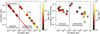Fig. 3 Predicted water vapor mass and its mass ratio relative to the solid mass as a function of CO mass in the left and right panels, respectively. All the symbols are defined in Fig. 2. As an example, the H2O-to-CO conversion factor is switched from Eq. (12) for Hypothesis 1 to Eq. (14) for Hypothesis 2 at the transition CO mass of 10–3; for clear comparison, these conversion factors are shown by the solid red and the dashed orange lines for Hypotheses 1 and 2, respectively (left panel). Such switching results in a clear jump in the H2O mass and its mass ratio. In the left panel, tentative constraints derived from previous observations are also plotted; the water vapor mass estimated for the protoplanetary disk around TW Hydrae is denoted by the horizontal, solid red line segment, while that for the debris disk around β Pic is represented by the error bar. The non-monotonic distributions in the water vapor mass and its mass ratio relative to the solid mass enable better determination of the origin of gas in debris disks.

3 Summary and outlook

Revealing the origin of gas in debris disks is one outstanding issue in understanding the time evolution of planet-forming disks. In the literature, two competing hypotheses are proposed (i.e., primordial origin vs. secondary origin; Fig. 1). Current observations of CO gas alone cannot reliably distinguish between these hypotheses (Fig. 2). We demonstrate through order-of-magnitude analyses that cold water vapor can play such a differentiating role. This becomes possible because the abundance of water vapor differs considerably between these two hypotheses (Eq. (12) vs. Eq. (14)). The resulting distribution of water mass as a function of CO mass shows non-monotonic behavior (Fig. 3), which can be used to better specify when the relative importance of these hypotheses would switch. This work therefore demonstrates that detection of cold water vapor is key to shedding light on the origin of gas in debris disks.

However, observations of cold water vapor are not possible with currently available telescopes. To illustrate this, Fig. 4 shows emission lines from water vapor as a function of wavelength. It is clear that most lines originating from low excitation temperatures fall in the FIR range. Such a wavelength range may become accessible in the future, thanks to the recent astrophysics probe call by NASA, i.e., the 2023 Astrophysics Probe Explorer (APEX). This work strongly supports the case for development of a future FIR space observatory.

Historically, such wavelengths were covered by Herschel. While a number of debris disks were observed by the space telescope (e.g., Eiroa et al. 2013; Booth et al. 2013), no claim was made in literature that cold water vapor was discovered in these disks. This is probably because of the sensitivity issue; as described above, Herschel detected water vapor in the pro- toplanetary disk around TW Hydrae. A similar value for the water vapor mass would be possible for CO-gas-rich debris disks (Fig. 3). Non-detections might therefore be explained by the fact that, while TW Hydrae is about 60 pc away, these gas-rich debris disks are >100 pc away, resulting in the observable flux decreasing by a factor of 4 or more as a result of beam dilution. In order to reliably detect cold water vapor in debris disks and carefully examine its origin, a desired sensitivity improvement factor over Herschel for a future FIR instrument would be 100 or more.

We chose to adopt the simplified approach in this work as the detection of water vapor in debris disks remains to be performed. Our assumption likely holds for typical debris disks (Appendix A) and our results are promising for future observations. However, more detailed work is required to confirm our findings. It is critical to identify how much gas is released at what size of solids; if debris disks are massive enough (i.e., M_Z,ref > 0.1 M_⊕; see Appendix A), then different production and destruction processes may become dominant, such that the resulting water vapor abundance could be very low. In addition, simultaneous calculations of disk evolution and chemistry are key for Hypothesis 1, while coupling of calculations of gas production from collisions with disk chemistry is crucial for Hypothesis 2. We have shown that our abundance estimates would be valid for both interstellar and stellar UV radiation (Appendix B). However, the lifetime of water vapor depends on the UV source: if stellar UV radiation dominates, the lifetime could be very short and the detection of water vapor may be challenging. For this case, observations of OH, which is the outcome of photodissociation of water, may be used to infer the abundance of water vapor (Tabone et al. 2021; Zannese et al. 2024). Clearly, more dedicated investigations still need to be undertaken in future work.

In conclusion, modeling and detections of various molecules shed light on the origin of gas in debris disks. This work puts the particular focus on cold water vapor.

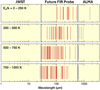Fig. 4 Emission lines from water vapor as a function of wavelength. The excitation temperature increases from the top to the bottom panels. Different observatories cover different wavelengths; this plot confirms that water lines detected by JWST come from high excitation temperatures (≳1000 K, i.e., hot (or warm) water). A future FIR space observatory would be the most sensitive to cold water vapor. A spectral resolution of R approximately equal to a few thousand appears to be sufficient for detections.

Acknowledgements

The authors thank an anonymous referee for the useful comments on our manuscript. This research was carried out at the Jet Propulsion Laboratory, California Institute of Technology, under a contract with the National Aeronautics and Space Administration (80NM0018D0004) and funded through the internal Research and Technology Development program as well as the NASA Exoplanets Research Program through grant 23-XRP23_2-0128. Y.H. is supported by JPL/Caltech. D.C.L. acknowledges financial support from the National Aeronautics and Space Administration (NASA) Astrophysics Data Analysis Program (ADAP).

Appendix A Production and destruction timescales of water vapor in debris disk-like environments

Here, we briefly discuss production and destruction timescales of water vapor in debris disk-like environments. We adopt typical values of debris disk parameters to compute these timescales; a disk is located R ~ 100 au away from the host star, its vertical thickness is h ~ 6 %, and its radial extent is ∆R ~ 50 au (e.g., Hughes et al. 2018). We show below that the assumption adopted in this work likely holds for such a typical debris disk, that is, in the debris disk-like environment, the water vapor abundance is regulated by competition between photodesorption and photodissociation. Most quantities are defined in the main text.

Water vapor is produced by both vaporization of water ice by destructive collisions and photodesorption. In Sect. 2.4, detailed collision properties and the resulting production rate are not considered. This is motivated by the assumption that the steady state collisional cascade might keep the water vapor abundance sufficiently high, so that detailed collision properties might not affect the abundance considerably. In contrast to protoplanetary disks, however, water vapor may be produced by collisions between small dust grains in debris disks. We estimate the corresponding timescale and compare it with the timescale of photodesorption.

The collision timescale between dust grains is estimated as $${\tau }_{\text{coll }}~\frac{1}{n_{\text{dust}}{\sigma }_{\text{dust}}{v}_{\text{rel}}},$$(A.1)

where n_dust = N_dust/(2πR²∆Rh) is the number density of dust particles distributed in debris disks, v_rel = ev_Kep is the relative velocity between the particles, e ~ 2h is the corresponding eccentricity, and v_Kep is the Keplerian velocity at R. Adopting the typical disk parameters described above, τ_coll becomes $$\begin{array}{c}{\tau }_{\text{coll }}\simeq 3.7\times {10}^2\text{yr}{\left(\frac{R}{100\text{\hspace{0.17em}au}}\right)}^{5/2}\left(\frac{\text{Δ}R}{50\text{\hspace{0.17em}au}}\right)\\ \times {\left(\frac{M_{Z,\text{ref}}}{{10}^{-1}{M}_{\oplus }}\right)}^{-1}\left(\frac{r_{\text{dust }}}{1\mu \text{m}}\right),\end{array}$$(A.2)

where M_Z,ref is estimated at ${\overline{M}}_{\text{CO,tran }}$ (Fig. 2).

If the water vapor abundance is regulated by competition between photodesorption and photodissociation as assumed in Sect. 2.4, then the timescale of photodesorption (τ_deso) becomes comparable to that of photodissociation (τ_diss), that is, $${\tau }_{\text{deso }}\sim {\tau }_{\text{diss }}\sim \frac{1}{R_0}\sim 3.2\times 10\text{\hspace{0.17em}yr}.$$(A.3)

This is a conservative upper limit as interstellar UV radiation is considered (see Appendix B).

Thus, we find τ_deso < τ_coll for typical debris disk-like environments.

On the other hand, water vapor is destroyed by both photodissociation and freeze-out onto dust grains. The freeze-out timescale is estimated as $${\tau }_{\text{free }}~\frac{1}{n_{\text{dust}}{\sigma }_{\text{dust}}{c}_{\text{s}}},$$(A.4)

where c_s is the sound speed of water vapor. Adopting the typical disk parameters, τ_free becomes $$\begin{array}{c}{\tau }_{\text{free }}\simeq 2.1\times {10}^2\text{yr}{\left(\frac{R}{100\text{\hspace{0.17em}au}}\right)}^2\left(\frac{\text{Δ}R}{50\text{\hspace{0.17em}au}}\right)\\ \times {\left(\frac{M_{Z,\text{ref}}}{{10}^{-1}{M}_{\oplus }}\right)}^{-1}{\left(\frac{T_{\text{gas}}}{100\text{\hspace{0.17em}K}}\right)}^{-1/2}\left(\frac{r_{\text{dust }}}{1\mu \text{m}}\right),\end{array}$$(A.5)

where M_Z,ref is again estimated at ${\overline{M}}_{\text{CO},\text{tran}}$ (Fig. 2), and the water vapor temperature is assumed to be 100 K.

Thus, we find τ_diss < τ_free for typical debris disk-like environments.

In summary, the assumption that the water vapor abundance is determined by competition between photodesorption and photodissociation likely holds for debris disks that have typical disk parameters. It should be noted that for debris disks with M_z,ref > 0.1 M_⊕ (or ${\overline{M}}_{\text{CO}}>{10}^{-3}{M}_{\oplus }$), both τ_coll and τ_free can become shorter than τ_deso and τ_diss, respectively. For this case, the assumption becomes no longer valid, and the water vapor abundance could be very low. However, the current observations confirm that debris disks whose observed CO gas can be explained by Hypothesis 2, satisfy the condition that M_Z,ref < 0.1 M_⊕ (or ${\overline{M}}_{\text{CO}}<{10}^{-3}{M}_{\oplus }$).

Appendix B The effect of stellar UV radiation

Here, we briefly discuss the effect of stellar UV radiation on the abundance estimate and lifetime of water vapor. We show below that our abundance estimates do not change very much even if the stellar UV radiation is included, but target-dependent calculations are needed to reliably estimate the lifetime.

First, our calculations conducted in Sect. 2.4 focus on the interstellar UV radiation, given that the presence of CO gas is confirmed only for debris disks, where interstellar UV radiation plays a major role in photodissociation than stellar UV radiation (Kral et al. 2017). For this case, the abundance of cold water vapor becomes independent of the UV flux because the optical depth effect that is applied to both the production and destruction rates cancels out. As a result, only the photodissociation cross section (σ_photo) emerges in Eq. (10), which is a function of the UV spectrum.

Second, if stellar UV radiation dominates over interstellar UV radiation, then the abundance of cold water vapor again becomes insensitive to the UV flux for the same reason; the optical depth effect cancels out. In this case, one needs to adopt the value of σ_photo that is computed from stellar UV spectrum. Young stars are known to have excess UV emission, and specific resonance lines like Lyman α dominate the spectrum (e.g., Bergin et al. 2003). The value of σ_photo at the Lyman α line is ${\sigma }_{\text{photo }}^{\text{Stellar }}=1.2\times {10}^{-17} {\text{cm}}^2$ (van Dishoeck et al. 2006). Interestingly, this value is comparable to that of the cross section derived for interstellar UV radiation, resulting in similar abundance estimates of cold water vapor.

Third, if the contribution of stellar UV radiation becomes comparable to that of interstellar UV radiation, then it is possible to mathematically assume that the resulting contribution would be twice the former one (or the latter one). The resulting abundance estimate is a factor of two smaller than the case where either interstellar UV radiation or stellar UV radiation dominates.

It thus can be concluded that our abundance estimates do not change very much even if stellar UV radiation is taken into account.

On the other hand, the lifetime of cold water vapor depends on the UV radiation source. Given that most debris disks would be optically thin at a wide range of wavelengths, it would be reasonable to consider that the lifetime derived from unshielded interstellar UV radiation gives an upper limit, which is about 30 yrs (see Eq. (A.3)). If stellar UV radiation dominates over interstellar UV radiation, then target-dependent calculations are needed because the photodissociation rate becomes functions of both the position of debris disks and the optical depth computed along from the host star to the disks. The resulting lifetime could be much shorter; for instance, a previous study estimates the lifetime of water vapor to be only 3.5 days for the debris disk around β Pic (Cavallius et al. 2019). For such targets, detecting cold water vapor would be challenging.

In summary, our abundance estimates would be reasonable for both interstellar and stellar UV radiation, while feasibility of observing cold water vapor in debris disks depends on the UV radiation source; if stellar UV radiation dominates, then the detection of the vapor may be hard due to its short lifetime.

Appendix C Monte Carlo-based realization of the CO and water gas masses

Here, we briefly describe how Monte-Carlo-based realization of the CO and water gas masses is conducted.

As described in Sect. 2.4, it is key to statistically identify non-monotonic behavior of the water gas mass as a function of CO gas mass. On the left panel of Fig. 3, constant values of the conversion factor (i.e., Eqs. (12) and (14) for Hypotheses 1 and 2, respectively) are used. One may then wonder how many targets with what mass sensitivity of these gas species would be needed for statistical identification, if the values vary. This can be addressed by performing Monte-Carlo-based realization of the CO and water gas masses.

We adopt a simplified approach, wherein the CO gas mass of targets is assumed to be logarithmically uniform in the observed range (i.e., 10^–1 – 4 × 10^–7M_⊕) and the conversion factor is assumed to be log normal with the peak value described in Eqs. (12) and (14) for Hypotheses 1 and 2, respectively. We have confirmed that the resulting log normal distribution covers the mass ratio of water to CO gas found in our order-of-magnitude analysis (Table 1). Also, we assume that switching occurs at the CO gas mass of 10^–3M_⊕; we have adopted smooth transitions with the transition width of up to 5 × 10^–4M_⊕ and confirmed that the results do not change very much.

Figure C.1 shows our results. We consider two sample sizes: one is N = 10, and the other is N = 30. It should be noted that the total number of observed systems is about 20 currently. First, we confirm by eye that statistical identification of the nonmonotonic behavior is very likely possible if N ≥ 10. Second, given that statistical identification becomes reliable only if error bars of data points do not overlap, the mass sensitivity of CO gas should be an order of 10^–4 M_⊕ or lower for both sample sizes; equivalently, errors should be a factor of few (or more) smaller than measurement values. For water vapor, the mass sensitivity should be 10^–9M_⊕ or lower for N = 10 and 10^–8M_⊕ or lower for N = 30.

In actual observations, the gas mass is computed from flux measurements. Observed flux is a function of targets’ distance. As described in Sect. 3, CO-gas-rich debris disks are > 100 pc away from the Earth. Therefore, a desired sensitivity improvement factor over Herschel would be 100 or more.

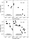Fig. C.1 Realization of the CO and water gas masses by the MonteCarlo approach. On the top panel, 10 realizations are done (i.e., 10 targets), while on the bottom panel, 30 realizations are performed. Statistical identification of the non-monotonic behavior is very likely possible if N ≳ 10 and if the mass sensitivities of CO gas and water gas are an order of 10–4M⊕ and of 10–9 – 10–8M⊕ or lower, respectively.

References

All Tables

All Figures

	Fig. 1 Schematic diagram of time evolution of planet-forming disks. The host star is denoted by the star symbol, planet-forming materials are represented by the brown and blue dots, and disk gas by the green ovals. Hypothesis 1 considers that observed gas is the leftover of primordial gas, while Hypothesis 2 considers that the gas is produced by collisions among icy bodies.
In the text

Fig. 2 Mass ratio of CO gas to solids as a function of CO gas mass. The theoretical estimates derived from the order-of-magnitude analysis are denoted by the solid red, dashed orange, and dotted black lines, respectively (see Eqs. (5), (9), and (1)). For comparison, the observed data are included (Moór et al. 2017, 2019; Di Folco et al. 2020; Rebollido et al. 2022); the circles represent targets that exhibit detections of both CO gas and dust, the triangles are for targets with dust-only detections (i.e., the upper limit for CO gas mass), and the diamonds are for targets with upper limits for both CO gas and dust. The color of each data point corresponds to the age of the target, as shown in the color bar on the right. Different disk parameters lead to different values of the CO-tosolid mass ratio (Table 1). The shaded red and orange regions represent possible ranges corresponding to Hypotheses 1 and 2, respectively. It is clear that the CO-to-solid mass ratio is not a reliable probe for tightly constraining the origin of the observed gas.

In the text

Fig. 3 Predicted water vapor mass and its mass ratio relative to the solid mass as a function of CO mass in the left and right panels, respectively. All the symbols are defined in Fig. 2. As an example, the H2O-to-CO conversion factor is switched from Eq. (12) for Hypothesis 1 to Eq. (14) for Hypothesis 2 at the transition CO mass of 10–3; for clear comparison, these conversion factors are shown by the solid red and the dashed orange lines for Hypotheses 1 and 2, respectively (left panel). Such switching results in a clear jump in the H2O mass and its mass ratio. In the left panel, tentative constraints derived from previous observations are also plotted; the water vapor mass estimated for the protoplanetary disk around TW Hydrae is denoted by the horizontal, solid red line segment, while that for the debris disk around β Pic is represented by the error bar. The non-monotonic distributions in the water vapor mass and its mass ratio relative to the solid mass enable better determination of the origin of gas in debris disks.

In the text

Fig. 4 Emission lines from water vapor as a function of wavelength. The excitation temperature increases from the top to the bottom panels. Different observatories cover different wavelengths; this plot confirms that water lines detected by JWST come from high excitation temperatures (≳1000 K, i.e., hot (or warm) water). A future FIR space observatory would be the most sensitive to cold water vapor. A spectral resolution of R approximately equal to a few thousand appears to be sufficient for detections.

In the text

Fig. C.1 Realization of the CO and water gas masses by the MonteCarlo approach. On the top panel, 10 realizations are done (i.e., 10 targets), while on the bottom panel, 30 realizations are performed. Statistical identification of the non-monotonic behavior is very likely possible if N ≳ 10 and if the mass sensitivities of CO gas and water gas are an order of 10–4M⊕ and of 10–9 – 10–8M⊕ or lower, respectively.

In the text

References

- Alexander, R., Pascucci, I., Andrews, S., Armitage, P., & Cieza, L. 2014, in Protostars and Planets VI, eds. H. Beuther, R. S. Klessen, C. P. Dullemond, & T. Henning (Tucson: University of Arizona Press), 475 [Google Scholar]
- Banzatti, A., Pontoppidan, K. M., Carr, J. S., et al. 2023, ApJ, 957, L22 [NASA ADS] [CrossRef] [Google Scholar]
- Bergin, E., Calvet, N., D’Alessio, P., & Herczeg, G. J. 2003, ApJ, 591, L159 [Google Scholar]
- Beust, H., Lagrange-Henri, A. M., Vidal-Madjar, A., & Ferlet, R. 1990, A&A, 236, 202 [NASA ADS] [Google Scholar]
- Biver, N., Bockelée-Morvan, D., Hofstadter, M., et al. 2019, A&A, 630, A19 [NASA ADS] [CrossRef] [EDP Sciences] [Google Scholar]
- Bolatto, A. D., Wolfire, M., & Leroy, A. K. 2013, ARA&A, 51, 207 [CrossRef] [Google Scholar]
- Bonsor, A., Wyatt, M. C., Marino, S., et al. 2023, MNRAS, 526, 3115 [NASA ADS] [CrossRef] [Google Scholar]
- Booth, M., Kennedy, G., Sibthorpe, B., et al. 2013, MNRAS, 428, 1263 [Google Scholar]
- Brandeker, A., Liseau, R., Olofsson, G., & Fridlund, M. 2004, A&A, 413, 681 [NASA ADS] [CrossRef] [EDP Sciences] [Google Scholar]
- Cataldi, G., Aikawa, Y., Iwasaki, K., et al. 2023, ApJ, 951, 111 [NASA ADS] [CrossRef] [Google Scholar]
- Cauley, P. W., France, K., Herzceg, G. J., & Johns-Krull, C. M. 2021, AJ, 161, 217 [NASA ADS] [CrossRef] [Google Scholar]
- Cavallius, M., Cataldi, G., Brandeker, A., et al. 2019, A&A, 628, A127 [NASA ADS] [CrossRef] [EDP Sciences] [Google Scholar]
- Choukroun, M., Altwegg, K., Kührt, E., et al. 2020, Space Sci. Rev., 216, 44 [CrossRef] [Google Scholar]
- Clarke, C. J., Gendrin, A., & Sotomayor, M. 2001, MNRAS, 328, 485 [NASA ADS] [CrossRef] [Google Scholar]
- Combi, M., Shou, Y., Fougere, N., et al. 2020, Icarus, 335, 113421 [NASA ADS] [CrossRef] [Google Scholar]
- Czechowski, A., & Mann, I. 2007, ApJ, 660, 1541 [NASA ADS] [CrossRef] [Google Scholar]
- Davidsson, B. J. R. 2021, MNRAS, 505, 5654 [NASA ADS] [CrossRef] [Google Scholar]
- Davidsson, B. J. R., Samarasinha, N. H., Farnocchia, D., & Gutiérrez, P. J. 2022, MNRAS, 509, 3065 [Google Scholar]
- Dent, W. R. F., Wyatt, M. C., Roberge, A., et al. 2014, Science, 343, 1490 [NASA ADS] [CrossRef] [Google Scholar]
- Di Folco, E., Péricaud, J., Dutrey, A., et al. 2020, A&A, 635, A94 [NASA ADS] [CrossRef] [EDP Sciences] [Google Scholar]
- Dominik, C., Ceccarelli, C., Hollenbach, D., & Kaufman, M. 2005, ApJ, 635, L85 [NASA ADS] [CrossRef] [Google Scholar]
- Du, F., & Bergin, E. A. 2014, ApJ, 792, 2 [NASA ADS] [CrossRef] [Google Scholar]
- Eiroa, C., Marshall, J. P., Mora, A., et al. 2013, A&A, 555, A11 [NASA ADS] [CrossRef] [EDP Sciences] [Google Scholar]
- Favre, C., Cleeves, L. I., Bergin, E. A., Qi, C., & Blake, G. A. 2013, ApJ, 776, L38 [Google Scholar]
- France, K., Herczeg, G. J., McJunkin, M., & Penton, S. V. 2014, ApJ, 794, 160 [NASA ADS] [CrossRef] [Google Scholar]
- Fulle, M., Blum, J., Green, S. F., et al. 2019, MNRAS, 482, 3326 [NASA ADS] [CrossRef] [Google Scholar]
- Grigorieva, A., Thébault, P., Artymowicz, P., & Brandeker, A. 2007, A&A, 475, 755 [NASA ADS] [CrossRef] [EDP Sciences] [Google Scholar]
- Habing, H. J. 1968, Bull. Astron. Inst. Netherlands, 19, 421 [Google Scholar]
- Harrington Pinto, O., Womack, M., Fernandez, Y., & Bauer, J. 2022, Planet. Sci. J., 3, 247 [NASA ADS] [CrossRef] [Google Scholar]
- Hobbs, L. M., Vidal-Madjar, A., Ferlet, R., Albert, C. E., & Gry, C. 1985, ApJ, 293, L29 [NASA ADS] [CrossRef] [Google Scholar]
- Hogerheijde, M. R., Bergin, E. A., Brinch, C., et al. 2011, Science, 334, 338 [Google Scholar]
- Hollenbach, D., Johnstone, D., Lizano, S., & Shu, F. 1994, ApJ, 428, 654 [NASA ADS] [CrossRef] [Google Scholar]
- Hollenbach, D., Kaufman, M. J., Bergin, E. A., & Melnick, G. J. 2009, ApJ, 690, 1497 [NASA ADS] [CrossRef] [Google Scholar]
- Hughes, A. M., Lieman-Sifry, J., Flaherty, K. M., et al. 2017, ApJ, 839, 86 [NASA ADS] [CrossRef] [Google Scholar]
- Hughes, A. M., Duchêne, G., & Matthews, B. C. 2018, ARA&A, 56, 541 [Google Scholar]
- Kral, Q., Wyatt, M., Carswell, R. F., et al. 2016, MNRAS, 461, 845 [NASA ADS] [CrossRef] [Google Scholar]
- Kral, Q., Matrà, L., Wyatt, M. C., & Kennedy, G. M. 2017, MNRAS, 469, 521 [NASA ADS] [CrossRef] [Google Scholar]
- Marino, S., Flock, M., Henning, T., et al. 2020, MNRAS, 492, 4409 [Google Scholar]
- Marschall, R., Markkanen, J., Gerig, S.-B., et al. 2020, Front. Phys., 8, 227 [NASA ADS] [CrossRef] [Google Scholar]
- Miotello, A., van Dishoeck, E. F., Williams, J. P., et al. 2017, A&A, 599, A113 [NASA ADS] [CrossRef] [EDP Sciences] [Google Scholar]
- Moór, A., Curé, M., Kóspál, Á., et al. 2017, ApJ, 849, 123 [Google Scholar]
- Moór, A., Kral, Q., Ábrahám, P., et al. 2019, ApJ, 884, 108 [CrossRef] [Google Scholar]
- Mumma, M. J., & Charnley, S. B. 2011, ARA&A, 49, 471 [NASA ADS] [CrossRef] [Google Scholar]
- Nakatani, R., Kobayashi, H., Kuiper, R., Nomura, H., & Aikawa, Y. 2021, ApJ, 915, 90 [NASA ADS] [CrossRef] [Google Scholar]
- Nakatani, R., Turner, N. J., Hasegawa, Y., et al. 2023, ApJ, 959, L28 [NASA ADS] [CrossRef] [Google Scholar]
- Öberg, K. I., Linnartz, H., Visser, R., & van Dishoeck, E. F. 2009, ApJ, 693, 1209 [Google Scholar]
- Rebollido, I., Ribas, Á., de Gregorio-Monsalvo, I., et al. 2022, MNRAS, 509, 693 [Google Scholar]
- Slettebak, A. 1975, ApJ, 197, 137 [NASA ADS] [CrossRef] [Google Scholar]
- Smirnov-Pinchukov, G. V., Moór, A., Semenov, D. A., et al. 2022, MNRAS, 510, 1148 [Google Scholar]
- Tabone, B., van Hemert, M. C., van Dishoeck, E. F., & Black, J. H. 2021, A&A, 650, A192 [NASA ADS] [CrossRef] [EDP Sciences] [Google Scholar]
- Trapman, L., Zhang, K., van’t Hoff, M. L. R., Hogerheijde, M. R., & Bergin, E. A. 2022, ApJ, 926, L2 [NASA ADS] [CrossRef] [Google Scholar]
- van Dishoeck, E. F., Jonkheid, B., & van Hemert, M. C. 2006, Faraday Discuss., 133, 231 [Google Scholar]
- Westley, M. S., Baragiola, R. A., Johnson, R. E., & Baratta, G. A. 1995, Nature, 373, 405 [Google Scholar]
- Willacy, K., & Langer, W. D. 2000, ApJ, 544, 903 [NASA ADS] [CrossRef] [Google Scholar]
- Wyatt, M. C. 2008, ARA&A, 46, 339 [Google Scholar]
- Zannese, M., Tabone, B., Habart, E., et al. 2024, Nat. Astron., 8, 577 [Google Scholar]
- Zuckerman, B., & Song, I. 2012, ApJ, 758, 77 [Google Scholar]
Historically, the unusual presence of atomic absorption lines in stellar spectra was claimed by Slettebak (1975).
For the secondary origin, another hypothesis proposed in the literature is that the observed gas originates either from evaporation of cometary bodies due to host stellar radiation (Beust et al. 1990) or from degassing of planetesimals, driven by radiogenic heating (Davidsson 2021; Bonsor et al. 2023).
Release mechanisms of CO gas remain uncertain. In the literature, photodesorption from collisionally produced dust grains (Grigorieva et al. 2007), vaporization of dust grains due to high velocity collisions (Czechowski & Mann 2007), and collisions between cometary bodies (Zuckerman & Song 2012) are proposed.
The presence of hot (or warm) water is confirmed by recent JWST observations, and its presence can be explained by sublimation (e.g., Banzatti et al. 2023).
We confirm in Appendix A that photodesorption and photodissociation are the dominant processes to determine the abundance of cold water vapor in typical debris disks.
These typical values would be reasonable for disks around T Tauri stars. For disks around Herbig Ae/Be stars, however, some deviation would be possible due to inefficient photoelectric heating. As a result, Hypothesis 1 may be preferred to better reproduce observational trends (e.g., Nakatani et al. 2023).
The lower abundance of CO ice than of water ice could suggest that the majority of comets in the Solar System formed within the CO snow line. For extrasolar environments, most debris disks are observed around 100 au away from the host star (e.g., Hughes et al. 2018). Under the optically thin assumption, the temperature at the location of debris disks becomes 28 K around G-type stars, which is higher than the CO freeze- out temperature. Adopting the abundance ratio inferred from Solar System comets would thus be a reasonable first step for extrasolar environments. On the other hand, if debris disks are located around 200 au, then the temperature goes down to ∼20 K and becomes comparable to the CO freeze-out temperature. For this case, the abundance ratio of CO ice to water ice may become comparable, and the differentiation discussed in Sect. 2.4 may be less clear.
The UV flux is often normalized in units of G0, where 1 G0 = 1.6 × 10⁻³ erg cm–2 s–1 is the flux integrated over the range from 6 to 13.6 eV (Habing 1968).