| Issue |
A&A
Volume 653, September 2021
|
|
|---|---|---|
| Article Number | A70 | |
| Number of page(s) | 16 | |
| Section | Extragalactic astronomy | |
| DOI | https://doi.org/10.1051/0004-6361/202141273 | |
| Published online | 09 September 2021 | |
Galaxy properties of type 1 and 2 X-ray selected AGN and a comparison among different classification criteria
1
Instituto de Fisica de Cantabria (CSIC-Universidad de Cantabria), Avenida de los Castros, 39005 Santander, Spain
e-mail: This email address is being protected from spambots. You need JavaScript enabled to view it.
2
Aix Marseille Univ. CNRS, CNES, LAM, Marseille, France
e-mail: This email address is being protected from spambots. You need JavaScript enabled to view it.
3
Institut Universitaire de France (IUF), France
4
National Observatory of Athens, V. Paulou & I. Metaxa, 15 236 Penteli, Greece
5
Department of Physics and Astronomy, Texas A&M University, 77843-4242 College Station, TX, USA
6
George P. and Cynthia Woods Mitchell Institute for Fundamental Physics and Astronomy, Texas A&M University, 77843-4242 College Station, TX, USA
7
Section of Astrophysics, Astronomy and Mechanics, Department of Physics, Aristotle University of Thessaloniki, 54 124 Thessaloniki, Greece
8
Centro de Astronomía (CITEVA), Universidad de Antofagasta, Avenida Angamos 601, Antofagasta, Chile
Received:
8
May
2021
Accepted:
20
June
2021
Abstract
We present analyses of host galaxy properties of type 1 and type 2 X-ray selected Active galactic nuclei (AGNs) in the XMM-XXL field, which have an available optical spectroscopic classification. We modelled their optical to far-infrared spectral energy distributions (SEDs) using the X-CIGALE code. X-CIGALE allows for the fitting of X-ray flux and accounts for the viewing angle of dusty torus and the attenuation from polar dust. By selecting matched type 1 and 2 sub-samples in the X-ray luminosity and redshift parameter space, we find that both types live in galaxies with similar star formation. However, type 2 AGN tend to reside in more massive systems (10.87−0.12+0.06 M⊙) compared to their type 1 counterparts (10.57−0.12+0.20 M⊙). In the second part of our analysis, we compare the spectroscopic classification with that from the SED fitting. X-CIGALE successfully identifies all spectroscopic type 2 sources either by estimating an inclination angle that corresponds to edge on viewing of the source or by measuring increased polar dust in these systems. Approximately 85% of spectroscopic type 1 AGN are also identified as such, based on the SED fitting analysis. There is a small number of sources (∼15% of the sample) that present broad lines in their spectra, but they show strong indications of obscuration, based on SED analysis. These could be systems that are viewed face on and have an extended dust component along the polar direction. The performance of X-CIGALE in classifying AGN is similar at low and high redshifts, under the condition that there is sufficient photometric coverage. Finally, the usage of optical/mid-IR colour criteria to identify optical red AGN (u − W3) suggests that these criteria are better suited for IR selected AGN and their efficiency drops for the low to moderate luminosity sources included in X-ray samples.
Key words: X-rays: galaxies / galaxies: active / quasars: supermassive black holes / galaxies: star formation / galaxies: fundamental parameters
© ESO 2021
1. Introduction
Active galactic nuclei (AGNs) play an important role in galaxy evolution. They are powered by accretion onto the supermassive black hole (SMBH) located at the centre of galaxies. The AGN-galaxy co-evolution is governed by SMBH feeding mechanism(s) and AGN feedback. To decipher this interplay between the active SMBH and its host galaxy, it is important to shed light on the AGN structure. One of the most important aspects of this pursuit is to understand the physical difference between obscured and unobscured AGN.
According to the simplest form of the unification model (e.g., Antonucci 1993; Urry & Padovani 1995; Nenkova et al. 2002; Hönig et al. 2006; Schartmann et al. 2008; Netzer 2015), AGN are surrounded by a dusty gas torus structure that absorbs radiation emitted from the nucleus, that is to say the SMBH and the accretion disc around it. This absorbed radiation is then re-emitted at larger (IR) wavelengths. In this scenario, the angle the AGN is observed determines whether the source is observed as obscured or unobscured. When the AGN is viewed face-on, then the source is classified as unobscured (type 1), while when the AGN is observed edge-on the source is characterised as obscured (type 2). Thus, the classification of AGN into different types is purely a geometrical effect. Although, more complex AGN structures have been proposed to explain, for example, the diversity of classifications at different wavelengths (e.g., X-ray versus optical classifications) under the unified scheme of AGN (e.g., Ogawa et al. 2021; Arredondo et al. 2021), the inclination angle remains the determinant factor for classifying obscured and unobscured AGN.
However, in the context of the evolutionary models, different AGN types are attributed to SBMH and galaxies being observed at different phases. The core idea of these models is that obscured AGN are observed during an early phase, when the SMBH is still weak and incapable of expelling the surrounding gas and dust that has been pushed towards the galactic centre. This material feeds the AGN that eventually becomes powerful enough to push the surrounding material away (e.g., Ciotti & Ostriker 1997; Hopkins et al. 2006; Somerville et al. 2008). Under this scheme, obscuration is not solely related to the AGN torus, but also to absorbing content at galactic scales (e.g., Circosta et al. 2019; Malizia et al. 2020).
Studying the two AGN populations can shed light on many different aspects of the AGN-galaxy interplay. Under the evolutionary scheme, studying the obscured and unobscured AGN populations has further implications regarding, for example, the relation between BH growth and the growth of the host galaxy and the lifetime of each classification type (e.g., Hickox et al. 2011; Ballantyne 2017). However, we first need to understand what is the nature of obscured and unobscured AGN, that is to say whether the two AGN types are a geometrical effect or represent different stages of galaxy evolution. A popular approach to answer this question is to compare the host galaxy properties of obscured and unobscured AGN. If the two AGN populations live in similar environments, this would provide support to the unification model whereas if they reside in galaxies of different properties, it would suggest that they are observed at different evolutionary phases.
Previous works have selected AGN at different wavelengths and have applied different obscuration criteria to classify sources. Most studies that examined the host galaxy properties of X-ray selected AGN and classified them into obscured and unobscured using X-ray criteria, for example the value of the hydrogen column density NH, agree that both X-ray absorbed and unabsorbed AGN live in galaxies with a similar stellar mass, M*, and star-formation rate, SFR, (Merloni et al. 2014; Masoura et al. 2021; Mountrichas et al. 2021b, but see Lanzuisi et al. 2017). Chen et al. (2015) used IR selected AGN in the Boötes field and classified their sources using optical/mid-IR colours. Their analysis shows that type 2 AGN have higher IR star formation luminosities (i.e., higher SFR) compared to type 1 AGN by a factor of ∼2. Zou et al. (2019) used X-ray AGN and classified them based on optical spectra, morphology, and optical variability. Their analysis shows that type 2 AGN reside in more massive systems than their type 1 counterparts. Although the results of Chen et al. (2015) cannot be directly compared to those from X-ray studies, since their AGN selection is different, the results of Zou et al. (2019) suggest that although host galaxy properties are similar for X-ray absorbed and unabsorbed AGN, spectroscopically obscured X-ray sources reside in more massive systems than unobscured sources.
In this work, we use ∼2500 spectroscopic, X-ray selected AGN in the XMM-XXL field that have an available classification based on their optical spectra from the literature (Menzel et al. 2016). We applied spectral energy distribution (SED) fitting using the X-CIGALE code to measure the host galaxy properties of the two AGN types and compare them. In the second part of the analysis, we use the estimated inclination angle of each source from the SED fitting and compare it with the spectroscopic classification. Our goal is to examine the reliability of X-CIGALE classification and its effect on the accuracy on the measurements of the host galaxy properties. We also examine the efficiency of optical-IR colour criteria and specifically the u − W3 criterion of Hickox et al. (2017) in selecting obscured sources in an X-ray selected sample. Throughout this work, we assume a flat ΛCDM cosmology with H0 = 69.3 Km s−1 Mpc−1 and ΩM = 0.286.
2. Sample
We use spectroscopic X-ray AGN from the XMM-XXL field (Pierre et al. 2016). XXL is a medium depth X-ray survey, with a sensitivity of ∼6 × 10⁻¹⁵ erg cm −2 s−1 in the [0.5–2] keV band for point-like sources and an exposure time of about 10 ks per XMM pointing. It consists of two 25 deg2 extragalactic fields. The data used in this work come from the equatorial sub-region of the XXM-XXL North. In this field, 8445 X-ray sources have been observed. In addition, 5294 have SDSS counterparts, and spectroscopic redshifts are available for 2512 sources. The catalogue is presented in detail in Menzel et al. (2016).
In our analysis, we use 2512 spectroscopic X-ray selected AGN that lie within a redshift range of 0 < z < 5 (94% are at z < 2.5). The available photometry is described in Sect. 2 of Mountrichas et al. (2021a). In brief, in addition to the optical (SDSS) photometry available, the sources also have near-IR and mid-IR photometry from the Visible and Infrared Survey Telescope for Astronomy (VISTA; Emerson et al. 2006) and the allWISE (Wright et al. 2010) datasets. We also used catalogues produced by the HELP1 Collaboration to complement our mid-IR photometry with Spitzer (Werner et al. 2004) observations, and we added far-IR counterparts. Only the MIPS and SPIRE fluxes were considered, given the much lower sensitivity of the PACS observations for this field (Oliver et al. 2012). The W1 and W2 photometric bands of WISE nearly overlap with IRAC1 and IRAC2 from Spitzer. When a source had been detected by both IR surveys, we only considered the photometry with the highest signal-to-noise ratio (S/N). Similarly, when both W4 and MIPS photometry was available, we only considered the latter due to the higher sensitivity of Spitzer compared to WISE.
Robust measurements of galaxy properties are essential in our analysis. For this reason, we require sources to have the following photometry available: u, g, r, i, z, W1 or IRAC1, W2 or IRAC2, W3, and W4 or MIPS1. The resulted sample consists of 2,134 sources. Ultraviolet (UV) photometry allows one to trace the young stellar population. At z > 0.5, the u optical band is redshifted to the rest-frame wavelength < 2000 Å, allowing for an observation of the emitted radiation from young stars. At z < 0.5, shorter wavelengths are required (e.g., GALEX). GALEX photometric data are available for only 216 out of the 2512 X-ray sources (∼8%). Since the vast majority of AGN does not have GALEX photometry, we chose not to include it in the construction of the SEDs. Therefore, at z < 0.5, in the absence of UV photometry, we only kept sources that have available Herschel photometry. This reduces the number of sources to 1897. Finally, we excluded sources that do not have reliable optical spectral classifications from our analysis (for details see Sect. 4). This results in 1577 X-ray selected AGN.
3. Analysis
In this section, we describe the SED fitting analysis we followed to measure galaxy properties. We present our criteria to select only those sources with robust calculations of galaxy properties that are included in our final sample. Finally, we examine the reliability of the SED fitting measurements.
3.1. SED analysis using X-CIGALE
We measured the host galaxy properties of X-ray AGN in our sample by applying an SED fitting using the X-CIGALE code (Yang et al. 2020). X-CIGALE is a newly developed branch of the CIGALE fitting code (Boquien et al. 2019) that adds some important new features. The new algorithm has the ability to account for extinction of the UV and optical emission in the poles of AGN and it models the X-ray emission of galaxies. For the latter, it requires the intrinsic X-ray fluxes, that is, X-ray fluxes corrected for X-ray absorption. The improvements that these new features add in the fitting process are described in detail in Yang et al. (2020) and Mountrichas et al. (2021a).
For the SED fitting process, we used the intrinsic X-ray fluxes estimated in Mountrichas et al. (2021a). These measurements are based on hardness ratio estimations, calculated via a Bayesian approach called Bayesian Estimation of Hardness Ratios code (BEHR; Park et al. 2006). The details are presented in Sect. 3.1 of Mountrichas et al. (2021a). X-CIGALE uses the αox − L2500 Å relation of Just et al. (2007) to connect the X-ray flux with the AGN emission at 2500 Å. We adopted a maximal value of |Δαox|max = 0.2 that accounts for a ≈2 σ scatter in the above relation. The photon index, Γ, that is to say the slope of the X-ray spectrum, was set to 1.8.
AGN emission was modelled using the SKIRTOR templates (Stalevski et al. 2012, 2016). SKIRTOR assumes a clumpy two-phase torus model, based on 3D radiation-transfer. The model presented in Stalevski et al. was used for the UV to far-IR AGN emission with some modifications: the accretion disc was updated with the SED of Feltre et al. (2012) and dust emission and extinction was added in the poles of the AGN. For more details we refer to Yang et al. (2020). The AGN fraction is defined as the ratio of the AGN IR emission to the total IR emission of the galaxy, that is, the integrated luminosity from 8-1000 μm in rest-frame. The extinction due to polar dust was modelled as a dust screen geometry and a grey-body dust re-emission. The amount of extinction was measured with the EB − V parameter. We adopted the Small Magellanic Cloud (SMC) extinction curve (Prevot et al. 1984). Re-emitted grey-body dust was parameterised with a temperature of 100 K and emissivity index of 1.6. The dust temperature likely has a wide distribution, but its effect on the SED fitting parameters is minimal (Mountrichas et al. 2021a, Buat et al., in prep.). The galaxy component was fitted using a delayed star formation history (SFH) with the functional form SFR ∝t × exp(−t/τ). A star formation burst was also considered and modelled as constant, ongoing star formation no longer than 50 Myr. The burst was superimposed to the delayed SFH (Buat et al. 2019). Stellar emission was modelled using the Bruzual & Charlot (2003) single stellar populations template. The initial mass function (IMF) of Chabrier (2003) was adopted. Metallicity was fixed to 0.02. Stellar emission was attenuated following the Charlot & Fall (2000) recipe. We adopted a value of μ = 0.5, where μ is the ratio of the total attenuation undergone by stars older than 10 Myr to that undegone by stars younger than 10 Myr (Małek et al. 2018; Buat et al. 2019). The IR SED of the dust heated by stars was implemented with the Dale et al. (2014) library, without the AGN component. The modules and input parameters we use in our analysis are presented in Table 1.
Models and the values for their free parameters used by X-CIGALE for the SED fitting of our galaxy sample.
3.2. Selection of galaxy SEDs with secure fits
For each parameter estimated via SED fitting, the algorithm provides two estimates. One is calculated using the best-fit model (best value) and the other estimate of a parameter corresponds to the likelihood weighted mean value measured from its probability density function marginalised over all the other parameters (bayes value). The weight is based on the likelihood, exp (−χ2/2), associated with each model (Boquien et al. 2019). A large difference between these two values is an indication that the probability density function (PDF) is asymmetric or multi-peaked. Therefore, to exclude sources with unreliable SFR and M* measurements from our analysis, we considered only X-ray sources with  and
and  , where SFRbest and M*, best are the best fit values of SFR and M*, respectively, and SFRbayes and M*, bayes are the Bayesian values, estimated by X-CIGALE. These criteria reduce the number of X-ray sources to 1292 (from 1577). The choice of the limits is empirical. Allowing for more strict or loose lower and upper boundaries, for example, 0.1 − 0.33 and 3 − 10 changes the size of our catalogue by less than ±0.1% and thus does not affect our results and conclusions. Additionally, 91 sources (≈7% of the sample) with
  are excluded from our analysis (see appendix for more details). Figure 1 presents examples of SEDs from sources that satisfy the aforementioned criteria. Finally, among the 1201 (1292–91) AGN, we only consider sources with SFR and M* measurements that have a statistical significance of S/N > 2. The S/N is defined as
  , where the error in the denominator is the error of the parameter, estimated by X-CIGALE. This requirement reduces the AGN sample further and is discussed in more detail in Sect. 4.2. The combination of these selection criteria allows us to compare host galaxy properties of spectroscopic type 1 and 2 X-ray AGN, using only sources with the most robust host galaxy properties measurements.
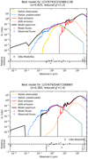 |
Fig. 1. Examples of SEDs from sources that satisfy our selection criteria (see Sect. 3.2). A source classified as type 1 based on SED fitting is presented in the top panel. A type 2 AGN is presented in the bottom panel (see text for more details on the SED classification). |
3.3. The effect of Herschel photometry
In our sample, 683 out of the 1201 X-ray sources (∼57%) have been observed by Herschel. For these sources, we ran X-CIGALE again, using the same parametric grid described in the previous section. However, in this second run, we did not take the far-IR photometric bands into account. Our goal is to examine the effect of Herschel photometry in the SFR measurements by comparing the SFR calculations of the two runs. The results are presented in Fig. 2. The two measurements are in very good agreement (SFRno Herschel = (0.99 ± 0.03) SFRHerschel + 0.12 ± 0.02). The distribution of the difference log SFRno Herschel − = log SFRHerschel has a mean value of μ = 0.10 and a dispersion of 0.33. Examining the results separately for spectroscopic type 1 (blue circles) and type 2 (red circles) yields SFRno Herschel = (0.89 ± 0.05) SFRHerschel + 0.23 ± 0.05 and SFRno Herschel = (1.02 ± 0.01) SFRHerschel + 0.12 ± 0.01, respectively. The distribution of the difference has a mean value of μ = 0.11, and 0.03 with a dispersion of 0.35 and 0.26 for type 1 and 2, respectively.
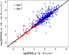 |
Fig. 2. Comparison of SFR measurements with and without Herschel photometry, for 683 X-ray sources that have available far-IR photometry. Spectroscopic type 1 sources are shown by blue circles, while type 2 sources are shown by red circles. The black solid line presents the 1:1 relation. Results show a very good agreement between the two measurements (SFRno Herschel = (0.99 ± 0.03) SFRHerschel + 0.12 ± 0.02). Examining the two AGN types separately yields SFRno Herschel = (0.89 ± 0.05) SFRHerschel + 0.23 ± 0.05 and SFRno Herschel = (1.02 ± 0.01) SFRHerschel + 0.02 ± 0.01, for type 1 and 2, respectively. |
Furthermore, we compared the values estimated by X-CIGALE for the Herschel fluxes with those from the data. The mean difference of log Herscheldata − log Herschelmodel is −0.02, −0.06, and 0.08, with a dispersion of 0.23, 0.25, and 0.33 for SPIRE250, SPIRE350, and SPIRE500, respectively. The results are similar for both AGN types. In Fig. 3, we present the comparison for SPIRE250. We also compared the reliability of the SFR measurements of those sources that have been observed by Herschel with those that do not have a Herschel detection. For that purpose, we used X-CIGALE’s ability to create and analyse mock catalogues. These catalogues are based on the best fit model of each source in the dataset. The algorithm uses the best model flux of each source and inserts noise, extracted from a Gaussian distribution with the same standard deviation as the observed flux. Then the mock data are analysed in the same way as the observed data (Boquien et al. 2019). We used the mock catalogues to compare the input and output values of this process and examined the precision of an estimated parameter. The mean difference of the estimated SFR of the mock sources from the input SFR values is 0.01 and 0.00 for the Herschel detected and non-detected sources, respectively, and the corresponding dispersions are 0.23 and 0.26.
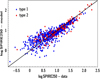 |
Fig. 3. Comparison of the values estimated by X-CIGALE with those from the data, for the SPIRE250 flux from Herschel. The mean difference log Herscheldata − log Herschelmodel is −0.02 with a dispersion of 0.23, regardless of the AGN type. |
Based on these results and the fact that X-ray sources detected by Herschel have similar properties (e.g., redshift, LX) with those non-detected by Herschel, we conclude that the SFR measurements of those sources in our sample that do not have Herschel photometry are reliable. Masoura et al. (2018) found that SFR calculations without Herschel photometry are systematically underestimated compared to SFR measurements including Herschel. Their X-ray sample consists of sources observed in XXL. However, there are important differences between the two studies. Different selection (photometric) criteria have been applied, the modules and the parametric grid used for the SED fitting is different and the sample used in Masoura et al. (2018) includes both spectroscopic and photometric sources.
4. Host galaxy properties of obscured and unobscured AGN classified based on optical spectra
In this section, we estimate the host galaxy properties of spectroscopic type 1 and 2 X-ray AGN. We selected those sources with the most robust measurements and then compared the SFR, M*, and SFRnorm of the two AGN populations; SFRnorm is defined as the ratio of the SFR of AGN to the SFR of star-forming main sequence (MS) galaxies with the same stellar mass and redshift (e.g., Mullaney et al. 2015; Masoura et al. 2018, 2021; Bernhard et al. 2019). The Schreiber et al. (2015) analytical formula was used for the calculation of the latter.
4.1. Properties of type 1 and type 2 X-ray AGN
For the estimation of SFR and M*, we applied an SED fitting using the grid described in Sect. 3.1. In this case, the inclination angle was fixed to the value that corresponds to the AGN type indicated by the optical spectra, that is, 30° for type 1 and 70° for type 2. In addition to the SFR and M* properties, we also compared the SFRnorm parameter of the two AGN types. For the latter, we used expression (9) of Schreiber et al. (2015). As mentioned in Mountrichas et al. (2021b), using an expression from the literature to calculate the SFR of star-forming MS galaxies and to compare it with the SFR of X-ray AGN to estimate SFRnorm, hints at a number of systematics. For example, different methods and/or (SED fitting) algorithms may be used in the estimation of SFR and different definitions of MS may be applied in different studies. Thus, we only wish to examine in a qualitative manner whether the SFRnorm parameter differs for different AGN classifications and not draw conclusions regarding the position of the two AGN types relative to the MS.
We split the X-ray sample into type 1 and type 2 sources, using optical spectra. This information is available in the public catalogue presented in Menzel et al. (2016). The classification rules are described in detail in Sects. 2 and 3 of Menzel et al. In brief, the optical spectroscopic follow-up was performed using the BOSS spectrograph of SDSS (Smee et al. 2013). The full width at half maximum (FWHM) was estimated for emission lines originating from different regions of the AGN (Hβ, MgII, CIII, and CIV). A source is classified as type 1 when an emission line has an FWHM larger than 1000 km s−1. In our analysis, we only use AGN with a reliable spectral classification, for example, sources with lines that have low significance due to a very strong host galaxy continuum contribution or very low signal-to-noise ratio spectra, which are classified as type 2 candidates in the Menzel et al. catalogue (NLAGN2cand) and are excluded from our analysis. Therefore, we consider only sources that are labelled as BLAGN1 (type 1) and NLAGN2 (type 2) in the catalogue of Menzel et al. (2016). From the 1201 X-ray sources in our dataset (see Sect. 3.2), 1109 are type 1 and 92 are type 2.
Redshift and X-ray luminosity distributions of the two populations are presented in Fig. 4. We noticed that there are no type 2 sources above z > 1. This is due to two effects. It is well known that the fraction of type 2 AGN decreases at higher luminosities (e.g., Merloni et al. 2014; Aird et al. 2015). Moreover, at z > 1.0, the magnitude of type 2 sources reaches rmodel = 22.5 mag and the host galaxy becomes too faint to be detected by SDSS images (Menzel et al. 2016). On the other hand, spectroscopic type 1 AGN are biased towards high luminosity sources since broad lines are harder to detect at lower luminosities. To compare the host galaxy properties of the two sub-samples, we first accounted for their different LX and redshift distributions. For that purpose, a weight was assigned to each source. For the calculation of the weight, we joined the redshift distributions and normalised each one by the total number of sources in each redshift bin (in bins of 0.1). The same process was repeated for the LX distributions (in bins of 0.1 dex). This gives us the PDF in this 2D (LX, redshift) space. The latter was used to weigh each source based on its redshift and X-ray luminosity (e.g., Mountrichas et al. 2016, 2021b; Masoura et al. 2021). In practice, this means that we restricted the redshift range of type 1 and 2 sources to 0.1 < z < 0.9 and the X-ray luminosity to 43.0 < log [LX,2−10 keV(ergs−1)] < 44.8. Or equally, that sources outside these redshift and luminosity ranges are assigned a zero weight. There are 284 X-ray AGN that satisfy these conditions; 220 are type 1 and 64 are type 2.
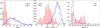 |
Fig. 4. Left and middle panels: redshift and LX distributions of type 1 and 2 AGN, among 1201 X-ray sources in our sample. The classification is based on optical spectra. Right panel: NH distribution for the 284 type 1 and 2 X-ray AGN that lie within the same redshift and LX range. |
The hydrogen column density, NH, quantifies the X-ray absorption of a source. This parameter has been estimated for all AGN in the Menzel et al. catalogue, in Liu et al. (2016). The NH have been calculated by applying X-ray spectral modelling and stacking, adopting the Bayesian X-ray Analysis software (BXA; Buchner et al. 2014) to fit the X-ray spectra of individual sources. The right panel of Fig. 4 presents the NH distributions of the two AGN types for the 284 AGN. The vast majority (90%) of type 1 sources are X-ray unabsorbed (NH < 1022 cm−2). On the other hand, optically classified type 2 AGN have a broad range of NH, split nearly equal between X-ray absorbed and unabsorbed sources. These trends (also seen in Fig. 9 of Liu et al. 2016) are consistent with those found in XMM-COSMOS (Merloni et al. 2014) and XMM-LSS (Garcet et al. 2007, see also Trouille et al. 2009). The NH measurements become less accurate for X-ray spectra with a low number of photons. Restricting the comparison of the NH distributions to sources with > 50 net photons does not change the results. This is also true if we were to replace the NH values from the Liu et al. catalogue with those estimated in Mountrichas et al. (2021a) that calculated NH, via hardness ratios, applying a Bayesian approach (Park et al. 2006). A possible scenario is that the observed trends are related to the large scatter that X-ray and optical obscuration present. This is due to, for example, X-ray column density variability (Yang et al. 2016), obscuration located at galactic scales that is not related to nuclear absorption (Malizia et al. 2020), and a complex AGN structure (Ogawa et al. 2021; Arredondo et al. 2021). There are studies that found X-ray absorbed sources with broad UV/optical lines (e.g., Li et al. 2019) and optical type 2 sources that have low X-ray absorption (e.g., Masoura et al. 2020).
4.2. Comparison of host galaxy properties of type 1 and 2 AGN
The estimation of host galaxy properties is more challenging for galaxies that host AGN compared to non-AGN systems. This is especially true for unobscured AGN. The AGN emission can outshine the optical emission of the host galaxy, thus increasing the uncertainties of the measurements. To estimate SFR, the SED code is, additionally, required to disentangle the IR emission of the host galaxy from the IR emission of the AGN. To examine the impact of these effects on the reliability of the SFR and M* measurements, we used the mock catalogues created by X-CIGALE. Figure 5 presents the results for the SFR (left panel) and M* (right panel) calculations for the 284 X-ray AGN. The vertical axis presents the Bayesian values of the parameter obtained from the fit of the mock sources, while the horizontal axis presents the true (input) values from the best fit of the data. Although, X-CIGALE successfully recovers the true SFR and M* values for most of the X-ray sources, there is a scatter, in particular in the M* measurements of type 1 AGN. To reduce this scatter, we estimated the statistical significance of each measurement and consider in our analysis only sources with the most robust measurements (S/N > 2). These sources are marked with an open circle in Fig. 5. Specifically, for the comparison of SFR between different AGN types, we kept only sources with (S/N)SFR > 2. Similarly, only sources with (S/N)M* > 2 are included in the comparison of the stellar mass distributions of the two populations. In the case of SFRnorm, both requirements were applied. This effectively reduces the scatter of the SFR and M* measurements. Table 2, presents the number of sources that satisfy the aforementioned criteria.
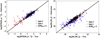 |
Fig. 5. Comparison of the SFR and M* measurements (left and right panel, respectively) for the estimated and true values from the mock analysis. Blue triangles show the results for type 1 X-ray AGN and red circles correspond to type 2 X-ray AGN. Sources are classified based on optical spectra. The black solid line shows the 1:1 relation. Restricting the measurements to those sources with statistical significance, §/N > 2 (open circles), effectively reduces the scatter of the calculations. |
Number of X-ray sources classified as type 1 and type 2, using optical spectra and SED fitting that have reliable SFR and M* measurements.
The SFR, stellar mass, and SFRnorm distributions of type 1 and 2 X-ray AGN are presented in Fig. 6. We note that for the comparison of the galaxy properties, the redshift and X-ray luminosity distributions of the various type 1 and 2 AGN sub-samples were matched by weighting each source, following the procedure described above. The two-sample Kolmogorov-Smirnov test (KS-test) and the Mann-Whitney test (MW-test), show that the SFR distributions (left panel) of the two populations are similar. The p − values are 0.77 and 0.47, respectively. The two tests show that the SFRnorm distributions are also similar (right panel; p − values = 0.82, 0.56, for the KS- and MW-test, respectively). However, the M* distribution of type 2 X-ray AGN peaks at higher M* values, compared to their type 1 counterparts (middle panel). The difference is not statistically significant based on the KS- and MW-tests (p − values = 0.24, 0.17, respectively). We estimated the errors on the mean values, using bootstrap re-sampling (e.g., Loh 2008). The results are presented in Table 3. Based on these measurements, the difference in the stellar mass of type 1 and 2 X-ray AGN is ∼0.3 dex, but it is significant only at 1 σ. However, this difference is in agreement with previous studies. Zou et al. (2019) used optical spectra, morphology, and optical variability to classify X-ray sources in the COSMOS field into type 1 and type 2. Their results show no difference in the SFR distributions of the two populations. However, they found that type 1 AGN tend to live in galaxies with smaller, by 0.2 dex, stellar mass than their type 2 counterparts, at a significance of ≈4σ. Thus, both our study and that of Zou et al. (2019) find a very similar difference in the mean stellar mass of galaxies that host type 1 versus type 2 X-ray AGN. A possible reason that the result of Zou et al. (2019) has a higher statistical significance than ours is the additional criteria they applied to classify sources.
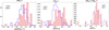 |
Fig. 6. From left to right: star formation rate, stellar mass, and SFRnorm distributions of type 1 (blue lines) and type 2 (red shaded histograms) X-ray selected AGN. The classification is based on optical spectra. We note that SFR and SFRnorm distributions of the two populations are similar. However, type 2 AGN tend to reside in galaxies with stellar mass ∼0.30 dex higher than type 1 AGN ( |
![Mathematical equation: $ \rm log\,[M_*(M_\odot)]=10.87^{+0.06}_{-0.12} $](/articles/aa/full_html/2021/09/aa41273-21/aa41273-21-eq7.gif)

Zou et al. (2019) suggest that the small difference in stellar mass between type 1 and type 2 AGN is related to the lower X-ray absorption of type 1 sources. Some previous studies found a correlation between NH and M* (Buchner et al. 2017; Lanzuisi et al. 2017). However, other X-ray studies found that X-ray absorbed and unabsorbed AGN live in galaxies with a similar stellar mass (Merloni et al. 2014; Masoura et al. 2021; Mountrichas et al. 2021b). In our sample, most type 1 sources have lower NH values (median of log [NH (cm−2) = 20.60) compared to type 2 sources (median of log [NH (cm−2)] = 21.49), but the distribution of the latter is very broad (Fig. 4).
We conclude that AGN classified as type 1 and 2 based on optical spectra have similar SFR and SFRnorm distributions. On the other hand, type 2 AGN live, on average, in more massive galaxies than their type 1 counterparts. Although this difference does not appear to be statistically significant, it is in agreement with previous studies.
5. Comparison of AGN classification using different criteria
In the second part of our analysis, we compare the AGN classification based on optical spectra with that from SED fitting. Our goal is to investigate the consistency of the classification of X-CIGALE compared to optical spectra and examine whether the performance of the SED fitting classification affects the accuracy of the measurements of the host galaxy properties. We also examine the efficiency and effectiveness of optical-IR colour compared to optical spectra and X-CIGALE source classification.
5.1. Classification of AGN based on X-CIGALE
5.1.1. X-CIGALE versus spectral classification and the effect of polar dust
One of the parameters of the AGN module estimated via SED fitting is the viewing angle, i, at which the source was observed. We split X-ray AGN into two types based on the value of the inclination angle and compared their X-CIGALE classification with that from optical spectra. We restricted the AGN sample to the 284 AGN that have a secure spectral classification and are within the same redshift and LX range (see Sect. 4). Examination of the mock catalogue reveals that X-CIGALE retrieves the i parameter within ±2° (mean value of the difference of the estimated to the true i values). The dispersion is 10°. In this exercise, we only considered AGN with a secure X-CIGALE classification. To identify these sources, we used the bayes and best estimates of the i parameter, derived by the SED fitting. Secure type 1 sources, based on X-CIGALE, are those with ibest = 30° and ibayes < 40°, while secure type 2 sources are those with ibest = 70° and ibayes > 60°. We note that 240 (∼85%) out of the 284 AGN have a secure classification from X-CIGALE; 187 are type 1 and 53 are type 2 AGN. The reasons for 44 sources not having a secure classification are investigated in the Appendix.
We also examine the classification performance of X-CIGALE for sources that lie at z > 1. Since there are no spectroscopic type 2 AGN at higher redshifts, we compared X-CIGALE’s classification with that from optical spectra only for type 1 sources. Our analysis shows that X-CIGALE classifies type 1 AGN with a similar efficiency both at z < 1 and z > 1, when sufficient photometric coverage is available. The details of this analysis are presented in the Appendix.
Figure 7 presents the redshift LX and NH distributions of the two AGN populations for the 284 sources. For comparison, we plotted the same distributions for type 1 and 2 sources based on optical spectra (dashed lines). The redshift and LX distributions of sources classified as type 1, based on X-CIGALE and optical spectra, are similar, peaking at higher redshifts and X-ray luminosities compared to their type 2 counterparts. The LX and redshift distributions of type 2 sources, based on SED fitting, appear flatter compared to spectroscopic type 2 AGN. The NH distribution of type 1 sources peaks at low NH values (NH < 1021 cm−2). The NH distribution of type 2 sources shows a second peak at NH > 1022 cm−2, which is similar to the NH distribution of type 2 sources, classified based on optical spectra (right panel of Fig. 4). As previously noted, broad line AGN that are obscured in X-rays have been reported in previous studies (e.g., Merloni et al. 2014).
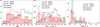 |
Fig. 7. Redshift LX and NH distributions of type 2 and type 1 AGN, based on the inclination angle estimated by X-CIGALE (red shaded area and blue line, respectively). For comparison, the distributions of type 1 and 2 sources, based on optical spectra, are also presented, with green and black dashed lines, respectively. |
Next, we compare the X-CIGALE classification with that from optical spectra, for the sample of 240 X-ray AGN. In the following, completeness refers to how many sources classified as type 1 (or type 2) based on optical spectroscopy were identified as such by the SED fitting results. The reliability is defined as the fraction of the number of type 1 (or type 2) sources classified by the SED fitting that are similarly classified by optical spectra.
Figure 8 presents the comparison of the two criteria. The SED fitting efficiently recovers the majority (160/188 = 85%, Table 4) of spectroscopic type 1 AGN. Moreover, most of the sources (160/187 = 86%) classified as type 1, based on the inclination angle estimates of X-CIGALE, were also identified similarly using optical spectra. The performance of SED fitting drops for type 2 sources. The reliability and completeness of X-CIGALE to uncover type 2 sources is 47% (25/53) and 48% (25/52), respectively (Table 4).
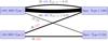 |
Fig. 8. Comparison of the classification of the 240 X-ray AGN in our dataset, using different classification criteria. The left side presents the number of sources classified based on SED fitting, while the right side shows the number of sources classified based on optical spectra. Numbers in the parentheses present the classification using the Hickox et al. (2017) criterion (the number of red sources is shown in red and non red sources is shown in blue). |
The ability of X-CIGALE to model and quantify the presence of polar dust in AGN has been shown to improve, for example, the AGN fraction estimates of the SED fitting (Mountrichas et al. 2021a). However, it makes the definition of obscured and unobscured sources more complex. Although polar dust does not affect the UV/optical SED of type 2 AGN, which is already absorbed by the dusty torus, it reddens the UV/optical SED of type 1 AGN. Thus, the polar dust model provides a physical explanation for red, type 1 AGN (Yang et al. 2020). Here, we examine how the addition of polar dust in the SED fitting process affects the comparison between X-CIGALE and spectral classification. First, we ran X-CIGALE without the ability of adding polar dust (EB − V = 0) for all 240 AGN, and we compared its classification with that of optical spectra. In this case, X-CIGALE securely classifies 214/240 AGN. Setting EB − V = 0.0 lowers the efficiency of X-CIGALE to identify spectroscopic type 1 sources to ∼61% (from 85% when polar dust is considered), and it increases it efficiency in recovering spectroscopic type 2 sources to 75% (from 48% when polar dust is considered). The percentages are shown in Table 4. We note that excluding the X-ray flux from the SED fitting process does not affect the classification of the sources.
There are 131 out of the 187 type 1 sources based on the inclination angle that have E(B − V),bayes > 0.15 (105/131 are also classified as type 1, based on optical spectra). This value corresponds to substantial extinction in the UV (∼50%), given the SMC extinction curve assumed for the SED modelling. For these sources, we examined whether the fits with polar dust are statistically different from those without polar dust. For that, we computed the Bayesian information criterion (BIC). The two fits were then compared using the ΔBIC parameter (e.g., Ciesla et al. 2018; Buat et al. 2019; Pouliasis et al. 2020). Only three sources show strong preference for polar dust based on the ΔBIC parameter (ΔBIC > 6.0). Forty-five out of the 131 AGN are classified as secure type 2 sources based on the inclination angle values, when polar dust is not considered; 15/45 are also spectroscopic type 2 (none has ΔBIC > 6.0). We conclude that a significant fraction (45/131 ≈ 35%) of type 1 (X-CIGALE) systems with increased polar dust could be securely classified as type 2 if polar dust is ignored, with the two classifications not differing statistically. Thus, in the following, when we examine sources that have a different classification from X-CIGALE and optical spectra, we take the effect of polar dust in these systems into account.
The comparison of the two classification criteria, presented in Fig. 8, reveals that there are 27 sources that are type 2 based on optical spectra, but they are classified as type 1 based on the SED fitting. There are also 28 sources that are spectroscopic type 1, but type 2 based on X-CIGALE. We examine these sources further to understand possible reasons for their different classification.
Comparison of classification of X-ray AGN, based on the inclination angle estimated by X-CIGALE and optical / mid-IR colours (Hickox et al. 2017) with respect to the classification using optical spectroscopy.
Among the 27 sources that are spectroscopic type 2, but type 1 based on the inclination angle of X-CIGALE, 26 have E(B − V),bayes > 0.15 and 15 are classified as type 2 when we ran X-CIGALE without the option of polar dust (EB − V = 0.0). Visual inspection of the SEDs of these 26 AGN showed that although they are classified as type 1 based on the inclination angle, their AGN emission presents (some) obscuration in the optical part of the spectrum. Figure 9 presents three examples of these cases. The SED of the one source out of the 27, that is type 1 and with E(B − V),bayes < 0.15, is presented in Fig. 10. We notice that although the  is lower than the threshold we set to exclude sources, optical photometry appears problematic, possibly due to blending with nearby, bright optical sources, and thus the fit from X-CIGALE is unreliable.
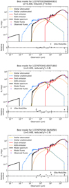 |
Fig. 9. Examples of SEDs of the 27 type 2 sources that are classified as unobscured, based on the inclination value estimated by X-CIGALE. We notice that their AGN emission presents (some) absorption in the optical part of the spectrum in agreement with their spectral classification. |
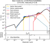 |
Fig. 10. SED of AGN that is spectroscopic type 2, but type 1 based on X-CIGALE and it does not have significant polar dust (E(B − V),bayes < 0.15). Although the |

Regarding the 28 X-ray AGN that are spectroscopic type 1, but type 2 based on X-CIGALE, 23 of them are systems with increased polar dust (E(B − V),bayes > 0.15). High values of polar dust in type 2 systems imply that there is a strong mid-IR emission detected in these systems. We ran X-CIGALE forcing the 28 sources to be type 1 (i = 30°). Based on ΔBIC, only two sources strongly favour (ΔBIC > 6.0) the fit with the run that has the free inclination angle. However, when the classification is forced to type 1 to match the spectral classification, polar dust, in most systems, increases further. Specifically, the mean E(B − V),bayes = 0.28 and E(B − V),bayes = 0.23, when i = 30° and i is free, respectively. Examples of the SEDs of these 28 AGN are presented in Fig. 11. Although these sources appear as type 1 based on the optical spectra, SED fitting analysis strongly suggests that these are absorbed systems. Merloni et al. (2014) found that a fraction of high luminosity AGN present broad lines in their optical spectra, but have absorbed X-ray spectra. The mean NH of the 28 sources is increased compared to that of the 160 AGN that are classified as type 1 based on both optical spectra and SED fitting (21.2 cm−2 versus 20.8 cm−2), but only 7/28 have NH > 21.5 cm−2. Previous studies have also reported similar cases of broad line X-ray AGN classified as type 2 based on SED fitting, without being necessarily X-ray absorbed (e.g., Masoura et al. 2020, see their Table 7 and figures in their Appendix). Different scenarios that allow a complex distribution of gas and dust in AGN have been suggested to explain the large variety of AGN properties (e.g., Lyu & Rieke 2018; Ogawa et al. 2021; Arredondo et al. 2021).
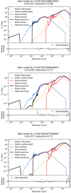 |
Fig. 11. Examples of SEDs of the 28 spectroscopic type 1 sources that are classified as type 2, i.e., dust obscured with a viewing angle of i = 70°, based on X-CIGALE. |
Overall, regarding the type 2 population of X-ray AGN, X-CIGALE identifies all of them, either as type 2 based on the inclination angle or as type 1 systems with increased polar dust. The only spectroscopically classified as type 2 source that has neither of the above, presents problematic optical photometry (Fig. 10). About the type 1 population of X-ray AGN, X-CIGALE identifies as type 1 160/188 sources. The 28 type 1 AGN that X-CIGALE classifies as type 2 could be systems with an extended, clumpy dust component along the polar direction.
5.1.2. The effect of X-CIGALE classification on the accuracy of host galaxy property measurements
In Sect. 4, we have examined the reliability of the SFR and M* measurements of the SED fitting, when the inclination angle of each source is fixed to a value based on the classification from optical spectra. Now, we use the 1201 X-ray sources in our dataset (see Sect. 3.2) and repeat the same exercise, setting the viewing angle free to examine whether the misclassification of X-CIGALE for some AGN affects the reliability of the calculations of the host galaxy properties. There are 972 (∼81%) sources with a secure classification from X-CIGALE; 681 are type 1 and 291 are type 2, based on SED fitting. We use the mock catalogues created by X-CIGALE and follow the procedure described in Sect. 4. Figure 12 presents the results. Sources that have S/N > 2 are presented by open circles. The number of X-ray AGN that satisfy the aforementioned criterion are shown in Table 2. We conclude, that although in this case the classification of AGN was not fixed and thus some sources are misclassified by X-CIGALE, this does not affect the reliability of the host galaxy measurements.
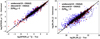 |
Fig. 12. Comparison of the SFR and M* measurements (left and right panel, respectively) for the estimated and true values from the mock analysis. Blue triangles show the results for type 1 X-ray AGN and red circles for type 2 X-ray AGN. Sources were classified using the value of inclination angle, estimated by the SED fitting. The black solid line shows the 1:1 relation. Restricting the measurements to those sources with statistical significance, S/N > 2 (open circles), effectively reduces the scatter of the calculations. |
5.2. Effectiveness of optical / mid-IR colours in classifying X-ray AGN
In this section, we discuss the performance of optical-IR colour criteria to detect obscured (type 2) AGN. The obscured AGN population is known to present very red optical-IR colours due to the extinction of the nuclear emission in (rest-frame) optical and UV wavelengths (e.g., Hickox et al. 2007). Although these colour criteria are very efficient in uncovering obscured AGN selected in the mid-IR, X-rays are known to miss a large fraction of obscured sources selected based on optical-IR colours. Mountrichas et al. (2020) used sources detected in Stripe 82 and found that among IR selected AGN with an SDSS detection, 43% are optically red. However, this percentage drops to 23% among those AGN that are also X-ray detected. Masoura et al. (2020) used data from the XMM-XXL and found that only ∼25% of red, IR selected AGN are detected in X-rays. Therefore, our X-ray selected AGN sample is biased against optical red sources.
Different optical-IR criteria exist in the literature that classify sources into obscured and unobscured. Yan et al. (2013) propose that red sources are identified using r − W2 > 6. However, this criterion is not sensitive at redshifts below z < 0.5 (Yan et al. 2013; Hickox et al. 2017). This is also true for other similar criteria (e.g., Hickox et al. 2007; LaMassa et al. 2016). Thus, we chose to apply an optical-IR criterion that effectively separates AGN into type 1 and 2 at all redshifts and most importantly at low redshift (z < 1) where our spectroscopic type 2 sources lie. Thus, we selected red AGN among the 240 X-ray sources (see Sect. 5.1.1) by applying the criterion presented in Hickox et al. (2017). Specifically, red sources were identified using u − W3 [AB] > 1.4(W1 − W2 [VEGA]) + 3.2.
The comparison of Hickox et al. (2017) optical-IR criteria with optical spectra is shown in Fig. 8 and Table 4. The colour criterion classifies many sources as red (138/240 ≈ 57%). It recovers most of the spectroscopic type 2 AGN, but also includes a large number of spectroscopic type 1 AGN. Only 32% (44/138) of red AGN are spectroscopically classified as type 2. Moreover, only half of type 1 sources are identified as non red systems (94/188). Hickox et al. (2017) find that the criterion identifies > 90% of spectroscopic type 1 and 2 AGN. We note that their sample consists of SDSS (luminous) quasars. Although, our sample, which consists of sources observed by SDSS, is X-ray selected and therefore includes sources with lower and moderate luminosities in addition to luminous AGN. We selected the most luminous sources in our sample by applying the following criteria: W1 − W2 > 0.7 and W2 < 15.05 (e.g., Stern et al. 2012). There are 11 and 67 spectroscopic type 2 and type 1 sources that satisfy these criteria, respectively. Hickox et al. criterion identifies 28 red and 50 non red sources. The first noticeable difference is that in this more luminous AGN sub-sample, the fraction of red sources is significantly lower (28/78 = 36%). This is expected since the fraction of obscured sources drops as the luminosity increases. Eight sources are both red and type 2, that is ∼73% of spectroscopy type 2 are also red, while 47/67 (∼70%) are type 1 and non red. These numbers are closer to the percentages of correct identifications quoted in Hickox et al. (2017). This indicates that optical-IR colours could be less effective in separating X-ray AGN into obscured and unobscured, compared to optically selected quasars and IR selected AGN. Infrared and optical selected AGN samples are dominated by luminous AGN (e.g., log [LX(ergs−1)] > 44) and a clear separation is observed between unobscured AGN, which are optically bright, and obscured AGN, for which we only observe their stellar emission. On the other hand, X-ray detected AGN include a large fraction of moderate to low luminosity AGN that blur the separation of optical magnitude distributions of the two AGN types (Georgakakis et al. 2020).
Figure 13 shows the colour-colour space diagram that Hickox et al. used to define their criterion (shown by the solid line). The plot was made using magnitudes from the data, that is, not those estimated by X-CIGALE during the SED fitting. Sources classified as red are shown in a red colour and lie on the right side of the solid line. AGN classified as type 2 from the SED fitting are shown in green, while those spectroscopically classified as type 2 are marked with open squares. Sources with EB − V > 0.15 are presented with triangles. Among the 138 sources classified as red by the Hickox et al. criterion, only 39 are type 2, based on X-CIGALE. However, most red sources are systems with an increased amount of polar dust (121/138 = 88%) because of the strong reddening of their optical continuum. In the remaining 99 AGN (138-39), only 22 are spectroscopically classified as type 2. We note that all these 22 sources have EB − V > 0.15, that is to say they are AGN despite being classified as type 1 by X-CIGALE, based on their inclination angle, they have increased polar dust. This can be, at least partially, attributed to the fact that different obscuration criteria are sensitive to different levels of obscuration (e.g., Mountrichas et al. 2019; Masoura et al. 2020). Finally, among the 28 sources that are spectroscopically classified as type 1, but as type 2 based on X-CIGALE (see previous section), 17 are red systems based on the colour criterion.
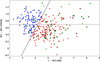 |
Fig. 13. Solid line splits the colour-colour diagram into red and non red AGN, using the Hickox et al. (2017) criterion. The horizontal dashed line indicates the W1 − W2 > 0.7 limit for the selection of IR AGN. Sources classified as optical red are shown in red, while the rest are shown in blue. AGN classified as type 2 from the SED fitting are presented in green. Sources with EB − V > 0.15 are shown with triangles. Sources spectroscopically classified as type 2 are marked by open squares. |
Our analysis is based on the SED fitting of individual AGN which increases the diversity of the examined cases. The inclusion of different stellar spectra and the ability to model the AGN absorption (polar dust) are some of the factors that increase the complexity and introduce degeneracies that could blur the boundaries of the locus that the two AGN populations occupy in the optical-IR colour space. The effect of polar dust on the AGN classification also depends on the adopted extinction curve and it could change significantly if a flatter extinction curve (e.g., Gaskell et al. 2004) were adopted instead of the SMC that is used in our analysis. Moreover, SED fitting requires good quality of photometric data and large wavelength coverage. In cases in which these criteria are not satisfactory met, the errors on the calculated fluxes can be quite large and the final fits do not necessarily reproduce the colours well. The effects of these factors will be investigated in an upcoming paper.
6. Summary
In this work, we study a sample of spectroscopic, X-ray selected AGN in the XMM-XXL field, which have type 1 and type 2 classifications based on their optical spectra from Menzel et al. (2016). Our goal is to examine the host galaxy properties of the two AGN populations and compare the spectroscopic classification of AGN with that from SED fitting.
To estimate the SFR and M*, we constructed SEDs for 1577 X-ray AGN, using optical to far-IR photometry. About half of the sources have been observed by Herschel. The SEDs were fit using the X-CIGALE code. X-CIGALE allows the inclusion of the X-ray flux in the fitting process and has the ability to account for extinction of the UV and optical emission in the poles of AGN by modelling polar dust. We restricted our analysis to those X-ray sources that meet our photometric criteria for available optical and mid-IR photometry, and those that have a secure optical classification and reliable estimates from the SED fitting.
The redshift and X-ray luminosities of spectroscopic type 1 and type 2 AGN present very different distributions (Fig. 4). To compare their host galaxy properties, we matched their LX and redshift distributions by weighting each source. This effectively reduced our sample to 284 sources. Our analysis reveals that both AGN populations live in galaxies with similar SFR and SFRnorm. The latter is defined as the ratio of the SFR of AGN to the SFR of star-forming MS galaxies with the same stellar mass and redshift. However, type 2 AGN tend to reside in more massive hosts compared to their type 1 counterparts. Specifically, the average stellar mass of type 1 host galaxies is  , compared to
  for type 2. Although, this result is statistically significant only at ≈1 σ, which is most likely due to the small examined sample, it is in agreement with previous studies (Zou et al. 2019).
One of the parameters estimated by the SED fitting process is the angle, i, that each AGN is observed. We compare the classification from X-CIGALE, based on the inclination angle, with that from optical spectra. X-CIGALE classifies as type 2 all spectroscopic type 2 sources, either by determining an edge on inclination angle or by measuring the increased presence of polar dust in these systems. The algorithm also successfully identifies the vast majority of type 1 sources (160/188 ≈ 85%). There are 28 type 1 sources that X-CIGALE securely classifies as type 2. Seven of them are also X-ray obscured (NH > 21.5 cm−2). Visual inspection of their SEDs shows that these AGN experience either strong absorption in the optical part of the spectrum and/or a large contribution of polar dust. Similar sources have also been found in previous studies (e.g., Merloni et al. 2014; Liu et al. 2018; Masoura et al. 2020). This class of AGN could be systems observed face on, which explains the presence of broad lines in their optical spectra with an extended dust component along the polar direction. This dust obscures the central SMBH causing an excess of mid-IR emission (Lyu & Rieke 2018). Similar results are found at z > 1, under the condition that sufficient and robust photometric data are available.
Finally, we compare the classification from SED fitting and optical spectra with that from optical-IR colours using the criteria of Hickox et al. (2017). Approximately 30% of red sources are identified as type 2 based on X-CIGALE/spectra. However, this percentage increases to ∼75% if we restrict the X-ray AGN sample to those sources that are also IR selected AGN (W1 − W2 > 0.7). Therefore, optical-IR colours seem to be more reliable at identifying obscured sources among IR selected AGN.
The Herschel Extragalactic Legacy Project (HELP; http://herschel.sussex.ac.uk/) is a European-funded project to analyse all the cosmological fields observed with the Herschel satellite. All the HELP data products can be accessed on HeDaM (http://hedam.lam.fr/HELP/).
Acknowledgments
The authors thank the anonymous referee for their detailed report that improved the quality of the paper. GM acknowledges support by the Agencia Estatal de Investigación, Unidad de Excelencia María de Maeztu, ref. MDM-2017-0765. The project has received funding from Excellence Initiative of Aix-Marseille University – AMIDEX, a French ‘Investissements d’Avenir’ programme. VAM and IG acknowledge support of this work by Greece and the European Union (European Social Fund-ESF) through the Operational Programme “Human Resources Development, Education and Lifelong Learning 2014-2020” in the context of the project “Anatomy of galaxies: their stellar and dust content though cosmic time” (MIS 5052455). MB acknowledges FONDECYT regular grant 1170618 XXL is an international project based around an XMM Very Large Programme surveying two 25 deg2 extragalactic fields at a depth of ∼6 × 10⁻¹⁵ erg cm −2 s−1 in the [0.5-2] keV band for point-like sources. The XXL website is http://irfu.cea.fr/xxl/. Multi-band information and spectroscopic follow-up of the X-ray sources are obtained through a number of survey programmes, summarised at http://xxlmultiwave.pbworks.com/. This research has made use of data obtained from the 3XMM XMM-Newton serendipitous source catalogue compiled by the 10 institutes of the XMM-Newton Survey Science Centre selected by ESA. This work is based on observations made with XMM-Newton, an ESA science mission with instruments and contributions directly funded by ESA Member States and NASA. Funding for the Sloan Digital Sky Survey IV has been provided by the Alfred P. Sloan Foundation, the US Department of Energy Office of Science, and the Participating Institutions. SDSS-IV acknowledges support and resources from the Center for High-Performance Computing at the University of Utah. The SDSS web site is www.sdss.org. SDSS-IV is managed by the Astrophysical Research Consortium for the Participating Institutions of the SDSS Collaboration including the Brazilian Participation Group, the Carnegie Institution for Science, Carnegie Mellon University, the Chilean Participation Group, the French Participation Group, Harvard-Smithsonian Center for Astrophysics, Instituto de Astrofísica de Canarias, The Johns Hopkins University, Kavli Institute for the Physics and Mathematics of the Universe (IPMU) / University of Tokyo, Lawrence Berkeley National Laboratory, Leibniz Institut für Astrophysik Potsdam (AIP), Max-Planck-Institut für Astronomie (MPIA Heidelberg), Max-Planck-Institut für Astrophysik (MPA Garching), Max-Planck-Institut für Extraterrestrische Physik (MPE), National Astronomical Observatories of China, New Mexico State University, New York University, University of Notre Dame, Observatário Nacional / MCTI, The Ohio State University, Pennsylvania State University, Shanghai Astronomical Observatory, United Kingdom Participation Group, Universidad Nacional Autónoma de México, University of Arizona, University of Colorado Boulder, University of Oxford, University of Portsmouth, University of Utah, University of Virginia, University of Washington, University of Wisconsin, Vanderbilt University, and Yale University. This publication makes use of data products from the Wide-field Infrared Survey Explorer, which is a joint project of the University of California, Los Angeles, and the Jet Propulsion Laboratory/California Institute of Technology, funded by the National Aeronautics and Space Administration. The VISTA Data Flow System pipeline processing and science archive are described in Irwin et al. (2004), Hambly et al. (2008) and Cross et al. (2012). Based on observations obtained as part of the VISTA Hemisphere Survey, ESO Program, 179.A-2010 (PI: McMahon). We have used data from the 3rd data release. This work is based [in part] on observations made with the Spitzer Space Telescope, which was operated by the Jet Propulsion Laboratory, California Institute of Technology under a contract with NASA.
References
- Aird, J., Coil, A. L., Georgakakis, A., et al. 2015, MNRAS, 451, 1892 [NASA ADS] [CrossRef] [Google Scholar]
- Antonucci, R. 1993, ARA&A, 31, 473 [Google Scholar]
- Arredondo, D. E., Martín, O. G., Dultzin, D., et al. 2021, A&A, 651, A91 [NASA ADS] [CrossRef] [EDP Sciences] [Google Scholar]
- Ballantyne, D. R. 2017, MNRAS, 464, 626 [NASA ADS] [CrossRef] [Google Scholar]
- Bernhard, E., Grimmett, L. P., Mullaney, J. R., et al. 2019, MNRAS, 483, L52 [CrossRef] [Google Scholar]
- Boquien, M., Burgarella, D., Roehlly, Y., et al. 2019, A&A, 622, A103 [NASA ADS] [CrossRef] [EDP Sciences] [Google Scholar]
- Bruzual, G., & Charlot, S. 2003, MNRAS, 344, 1000 [NASA ADS] [CrossRef] [Google Scholar]
- Buat, V., Ciesla, L., Boquien, M., Małek, K., & Burgarella, D. 2019, A&A, 632, A79 [CrossRef] [EDP Sciences] [Google Scholar]
- Buchner, J., Schulze, S., & Bauer, F. E. 2017, MNRAS, 464, 4545 [NASA ADS] [CrossRef] [Google Scholar]
- Buchner, J., Georgakakis, A., Nandra, K., et al. 2014, A&A, 564, A125 [NASA ADS] [CrossRef] [EDP Sciences] [Google Scholar]
- Chabrier, G. 2003, PASP, 115, 763 [Google Scholar]
- Charlot, S., & Fall, S. M. 2000, ApJ, 539, 718 [Google Scholar]
- Chen, C.-T. J., Hickox, R. C., Alberts, S., et al. 2015, AJ, 802, 50 [NASA ADS] [CrossRef] [Google Scholar]
- Ciesla, L., Elbaz, D., Schreiber, C., Daddi, E., & Wang, T. 2018, A&A, 615, A61 [NASA ADS] [CrossRef] [EDP Sciences] [Google Scholar]
- Ciotti, L., & Ostriker, J. P. 1997, AJ, 487, L105 [NASA ADS] [CrossRef] [Google Scholar]
- Circosta, C., Vignali, C., Gilli, R., et al. 2019, A&A, 623, A172 [NASA ADS] [CrossRef] [EDP Sciences] [Google Scholar]
- Cross, N. J. G., Collins, R. S., Mann, R. G., et al. 2012, A&A, 548, A119 [NASA ADS] [CrossRef] [EDP Sciences] [Google Scholar]
- Dale, D. A., Helou, G., Magdis, G. E., et al. 2014, ApJ, 784, 83 [NASA ADS] [CrossRef] [Google Scholar]
- Emerson, J., McPherson, A., & Sutherland, W. 2006, Msngr, 126, 41 [NASA ADS] [Google Scholar]
- Feltre, A., Hatziminaoglou, E., Fritz, J., & Franceschini, A. 2012, MNRAS, 426, 120 [Google Scholar]
- Garcet, O., Gandhi, P., Gosset, E., et al. 2007, A&A, 474, 473 [NASA ADS] [CrossRef] [EDP Sciences] [Google Scholar]
- Gaskell, C. M., Goosmann, R. W., Antonucci, R. R. J., & Whysong, D. H. 2004, AJ, 616, 147 [NASA ADS] [CrossRef] [Google Scholar]
- Georgakakis, A., Ruiz, A., & LaMassa, S. M. 2020, MNRAS, 499, 710 [CrossRef] [Google Scholar]
- Hambly, N. C., Collins, R. S., Cross, N. J. G., et al. 2008, MNRAS, 384, 637 [NASA ADS] [CrossRef] [Google Scholar]
- Hickox, R. C., Jones, C., Forman, W. R., et al. 2007, AJ, 671, 1365 [NASA ADS] [CrossRef] [Google Scholar]
- Hickox, R. C., Myers, A. D., Brodwin, M., et al. 2011, ApJ, 731, 117 [NASA ADS] [CrossRef] [Google Scholar]
- Hickox, R. C., Myers, A. D., Greene, J. E., et al. 2017, AJ, 849, 53 [NASA ADS] [CrossRef] [Google Scholar]
- Hönig, S. F., Beckert, T., Ohnaka, K., & Weigelt, G. 2006, A&A, 452, 459 [NASA ADS] [CrossRef] [EDP Sciences] [Google Scholar]
- Hopkins, P. F., Hernquist, L., Cox, T. J., et al. 2006, AJ, 163, 1 [NASA ADS] [Google Scholar]
- Irwin, M. J., Lewis, J., Hodgkin, S., et al. 2004, SPIE, 5493, 411 [Google Scholar]
- Just, D. W., Brandt, W. N., Shemmer, O., et al. 2007, ApJ, 685, 1004 [NASA ADS] [CrossRef] [Google Scholar]
- LaMassa, S. M., Civano, F., Brusa, M., et al. 2016, ApJ, 818, 88 [NASA ADS] [CrossRef] [Google Scholar]
- Lanzuisi, G., Delvecchio, I., Berta, S., et al. 2017, A&A, 602, A123 [NASA ADS] [CrossRef] [EDP Sciences] [Google Scholar]
- Li, J., Xue, Y., Sun, M., et al. 2019, AJ, 877, 5 [NASA ADS] [CrossRef] [Google Scholar]
- Liu, Z., Merloni, A., Georgakakis, A., et al. 2016, MNRAS, 459, 1602 [NASA ADS] [CrossRef] [Google Scholar]
- Liu, T., Merloni, A., Wang, J.-X., et al. 2018, MNRAS, 479, 5022 [NASA ADS] [CrossRef] [Google Scholar]
- Loh, J. M. 2008, ApJ, 681, 726 [CrossRef] [Google Scholar]
- Lyu, J., & Rieke, G. H. 2018, AJ, 866, 92 [NASA ADS] [CrossRef] [Google Scholar]
- Małek, K., Buat, V., Roehlly, Y., et al. 2018, A&A, 620, A50 [NASA ADS] [CrossRef] [EDP Sciences] [Google Scholar]
- Malizia, A., Bassani, L., Stephen, J. B., Bazzano, A., & Ubertini, P. 2020, A&A, 639, A5 [CrossRef] [EDP Sciences] [Google Scholar]
- Masoura, V. A., Mountrichas, G., Georgantopoulos, I., et al. 2018, A&A, 618, A31 [NASA ADS] [CrossRef] [EDP Sciences] [Google Scholar]
- Masoura, V. A., Georgantopoulos, I., Mountrichas, G., et al. 2020, A&A, 638, A45 [CrossRef] [EDP Sciences] [Google Scholar]
- Masoura, V. A., Mountrichas, G., Georgantopoulos, I., & Plionis, M. 2021, A&A, 646, A167 [EDP Sciences] [Google Scholar]
- Menzel, M.-L., Merloni, A., Georgakakis, A., et al. 2016, MNRAS, 457, 110 [NASA ADS] [CrossRef] [Google Scholar]
- Merloni, A., Bongiorno, A., Brusa, M., et al. 2014, MNRAS, 437, 3550 [NASA ADS] [CrossRef] [Google Scholar]
- Mountrichas, G., Georgakakis, A., Menzel, M.-L., et al. 2016, MNRAS, 457, 4195 [NASA ADS] [CrossRef] [Google Scholar]
- Mountrichas, G., Georgakakis, A., & Georgantopoulos, I. 2019, MNRAS, 483, 1374 [NASA ADS] [CrossRef] [Google Scholar]
- Mountrichas, G., Georgantopoulos, I., Ruiz, A., & Kampylis, G. 2020, MNRAS, 491, 1727 [CrossRef] [Google Scholar]
- Mountrichas, G., Buat, V., Yang, G., et al. 2021a, A&A, 646, A29 [EDP Sciences] [Google Scholar]
- Mountrichas, G., Buat, V., Yang, G., et al. 2021b, A&A, in press, https://www.doi.org/10.1051/0004-6361/202140630 [Google Scholar]
- Mullaney, J. R., Alexander, D. M., Aird, J., et al. 2015, MNRAS, 453, L83 [NASA ADS] [CrossRef] [Google Scholar]
- Nenkova, M., Ivezić, Ž., & Elitzur, M. 2002, AJ, 570, L9 [CrossRef] [Google Scholar]
- Netzer, H. 2015, ARA&A, 53, 365 [Google Scholar]
- Ogawa, S., Ueda, Y., Tanimoto, A., & Yamada, S. 2021, AJ, 906, 84 [NASA ADS] [CrossRef] [Google Scholar]
- Oliver, S. J., Bock, J., Altieri, B., et al. 2012, MNRAS, 424, 1614 [NASA ADS] [CrossRef] [EDP Sciences] [Google Scholar]
- Park, T., Kashyap, V. L., Siemiginowska, A., et al. 2006, AJ, 652, 610 [NASA ADS] [CrossRef] [Google Scholar]
- Pierre, M., Pacaud, F., Adami, C., et al. 2016, A&A, 592, A1 [NASA ADS] [CrossRef] [EDP Sciences] [Google Scholar]
- Pouliasis, E., Mountrichas, G., Georgantopoulos, I., et al. 2020, MNRAS, 495, 1853 [CrossRef] [Google Scholar]
- Prevot, M., Lequeux, J., Maurice, E., Prevot, L., & Rocca-Volmerange, B. 1984, A&A, 132, 389 [Google Scholar]
- Schartmann, M., Meisenheimer, K., Camenzind, M., et al. 2008, A&A, 482, 67 [NASA ADS] [CrossRef] [EDP Sciences] [Google Scholar]
- Schreiber, C., Pannella, M., Elbas, D., et al. 2015, A&A, 575, A74 [NASA ADS] [CrossRef] [EDP Sciences] [Google Scholar]
- Smee, S. A., Gunn, J. E., Uomoto, A., et al. 2013, AJ, 146, 32 [Google Scholar]
- Somerville, R. S., Hopkins, P. F., Cox, T. J., Robertson, B. E., & Hernquist, L. 2008, MNRAS, 391, 481 [NASA ADS] [CrossRef] [Google Scholar]
- Stalevski, M., Fritz, J., Baes, M., Nakos, T., & Popović, L. Č. 2012, MNRAS, 420, 2756 [NASA ADS] [CrossRef] [Google Scholar]
- Stalevski, M., Ricci, C., Ueda, Y., et al. 2016, MNRAS, 458, 2288 [NASA ADS] [CrossRef] [Google Scholar]
- Stern, D., Assef, R. J., Benford, D. J., et al. 2012, ApJ, 753, 30 [NASA ADS] [CrossRef] [Google Scholar]
- Trouille, L., Barger, A. J., Cowie, L. L., Yang, Y., & Mushotzky, R. F. 2009, AJ, 703, 2160 [NASA ADS] [CrossRef] [Google Scholar]
- Urry, C. M., & Padovani, P. 1995, PASA, 107, 803 [Google Scholar]
- Werner, M. W., Roellig, T. L., Low, F. J., et al. 2004, ApJS, 154, 1 [NASA ADS] [CrossRef] [Google Scholar]
- Wright, E. L., Eisenhardt, P. R. M., Mainzer, A. K., et al. 2010, AJ, 140, 1868 [Google Scholar]
- Yan, L., Donoso, E., Tsai, C.-W., et al. 2013, AJ, 145, 55 [NASA ADS] [CrossRef] [Google Scholar]
- Yang, G., Boquien, M., Buat, V., et al. 2020, MNRAS, 491, 740 [NASA ADS] [CrossRef] [Google Scholar]
- Yang, G., Brandt, W. N., Luo, B., et al. 2016, AJ, 831, 145 [NASA ADS] [CrossRef] [Google Scholar]
- Zou, F., Yang, G., Brandt, W. N., & Xue, Y. 2019, AJ, 878, 11 [CrossRef] [Google Scholar]
Appendix A: Sources with problematic photometry and unsecure X-CIGALE classification
From our analysis, we have excluded sources that have  (Sect. 3.2). Visual inspection of their SEDs shows that in these cases, there are some problematic photometric bands that did now allow a reliable fit. Fig. A.1 presents two examples of these SEDs.
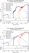 |
Fig. A.1. Examples of SEDs that have been excluded by our analysis due to their problematic photometry that results in unreliable SED fits ( |

We also investigate further the 44 sources that, although meeting our selection requirements, do not have a secure classification from the SED fitting (Sect. 5.1.1). Visual inspection of their SEDs reveals that X-CIGALE failed to provide a secure classification for at least one of the following reasons: one or more piece(s) of photometric data appear(s) inconsistent, resulting in increased  values, but lower than the threshold we set to exclude sources. The majority of these sources have a low(er) AGN fraction compared to the rest of the population (mean fracAGN = 0.28, compared to fracAGN = 0.43 for those with a secure classification). The UV/optical continuum is dominated by the stellar component, rendering it hard to distinguish between a type 2 AGN and a type 1 AGN with increased polar dust (see below for the effect of polar dust on the classification). The latter is, in particular true, for these systems with a low AGN fraction. Among the 44 AGN, 32 are spectroscopic type 1 and 12 are type 2. Sixteen out of the 32 have ibest = 30°, that is, X-CIGALE identifies them as type 1, which is in agreement with their spectroscopic classification, but not securely since ibayes > 40°. We fitted the remaining 16 sources again, forcing them to be type 1 AGN (i = 30°). All 16 sources have 2.0 < ΔBIC < 4.0. This suggests that there is no statistical difference in the SED fits, regardless of whether these sources are fitted as type 1 or type 2. The 12 sources that are type 2, but do not have a secure classification from their SED fitting, present similar results. Specifically, 5/12 have ibest = 70°. For the remaining seven, we ran X-CIGALE again and forced them to be type 2 (i = 70°) and compared the fits from the two runs. A ΔBIC analysis shows that there is no strong preference in favour of either of the two fits. We conclude that the X-CIGALE classification for these 44 AGN is ambiguous.
Appendix B: Classification of AGN based on X-CIGALE at z> 1
In the previous sections, we restricted our analysis to those sources that lie at z < 1. This was due to the fact that no AGN are classified as type 2 based on optical spectra at higher redshift (Sect. 4). In this section, we present the X-CIGALE classification of sources at z > 1 and compare it with spectroscopically classified type 1 AGN for which there is available information from the Menzel et al. (2016) catalogue.
There are 978 X-ray AGN that satisfy our photometric criteria, have a secure optical classification (Sect. 2), and  from their SED fitting. We note that 785 of them (∼80%) have a secure classification. This is similar to the fraction of sources that have a secure classification at z < 1 (∼85%, Sect. 5.1.1); 566 AGN are classified by X-CIGALE as type 1 and 219 are classified as type 2. Thus, the X-CIGALE classification agrees with that from optical spectra for 72% (566/785) of the sources. This number is somewhat lower compared to the percentage of sources that are classified as type 1, by X-CIGALE, and those that are also spectroscopic type 1, at z < 1 (160/188 ≈ 85%, Sect. 5.1.1).
We note that, at high redshifts, a larger fraction of sources is missing photometric data. Among the 240 AGN at z < 1 (Sect. 5.1.1), 80% have near-IR observations. However, at z > 1, 37% of the sources lack near-IR data (48% among the 219 that are classified as type 2, at z > 1, by X-CIGALE). Similarly, 75% of the 240 AGN have been observed by Herschel. This fraction drops to 55% at z > 1 and decreases further among the 219 AGN classified as type 2 (27%). It is also worth pointing out that the 219 AGN that are spectroscopic type 1, but classified as type 2 by X-CIGALE, lie at a mean redshift of z = 2.0, that is to say higher than that of the 566 sources that are classified as type 1, both from optical spectroscopy and SED fitting (z = 1.6).
We ran X-CIGALE forcing these 219 sources to be classified as type 1, in accordance with their spectroscopic classification. We then compared the fits from this run with that when the classification is free. For that, we estimated the ΔBIC parameter. With the exception of three sources that have ΔBIC > 6.0, ΔBIC varies from two to six, which indicates that the two fits do not differ statistically. Thus, the 219 AGN could also be classified as type 1, which is in agreement with their spectroscopic classification.
From the 219 sources, we selected 20 of them that satisfy the photometric criteria presented in Sect. 2 and additionally have near-IR and Herschel observations. Similarly to the results we found at z < 1, for the 28 spectroscopic type 1, X-ray AGN classified as type 2 by X-CIGALE, the majority of the sources (12/20) present increased polar dust (E(B − V),bayes > 0.15). The mean E(B − V),bayes increases from E(B−V),bayes = 0.12 to E(B − V),bayes = 0.19, when we forced these AGN to be fitted as type 1. Two sources have NH > 21.5 cm−2. We conclude that X-CIGALE can classify type 1 AGN at z > 1 with the same efficiency as at lower redshifts, under the condition that there is sufficient photometric coverage at high redshifts.
All Tables
Models and the values for their free parameters used by X-CIGALE for the SED fitting of our galaxy sample.
Number of X-ray sources classified as type 1 and type 2, using optical spectra and SED fitting that have reliable SFR and M* measurements.
Comparison of classification of X-ray AGN, based on the inclination angle estimated by X-CIGALE and optical / mid-IR colours (Hickox et al. 2017) with respect to the classification using optical spectroscopy.
All Figures
|
Fig. 1. Examples of SEDs from sources that satisfy our selection criteria (see Sect. 3.2). A source classified as type 1 based on SED fitting is presented in the top panel. A type 2 AGN is presented in the bottom panel (see text for more details on the SED classification). |
| In the text | |
|
Fig. 2. Comparison of SFR measurements with and without Herschel photometry, for 683 X-ray sources that have available far-IR photometry. Spectroscopic type 1 sources are shown by blue circles, while type 2 sources are shown by red circles. The black solid line presents the 1:1 relation. Results show a very good agreement between the two measurements (SFRno Herschel = (0.99 ± 0.03) SFRHerschel + 0.12 ± 0.02). Examining the two AGN types separately yields SFRno Herschel = (0.89 ± 0.05) SFRHerschel + 0.23 ± 0.05 and SFRno Herschel = (1.02 ± 0.01) SFRHerschel + 0.02 ± 0.01, for type 1 and 2, respectively. |
| In the text | |
|
Fig. 3. Comparison of the values estimated by X-CIGALE with those from the data, for the SPIRE250 flux from Herschel. The mean difference log Herscheldata − log Herschelmodel is −0.02 with a dispersion of 0.23, regardless of the AGN type. |
| In the text | |
|
Fig. 4. Left and middle panels: redshift and LX distributions of type 1 and 2 AGN, among 1201 X-ray sources in our sample. The classification is based on optical spectra. Right panel: NH distribution for the 284 type 1 and 2 X-ray AGN that lie within the same redshift and LX range. |
| In the text | |
|
Fig. 5. Comparison of the SFR and M* measurements (left and right panel, respectively) for the estimated and true values from the mock analysis. Blue triangles show the results for type 1 X-ray AGN and red circles correspond to type 2 X-ray AGN. Sources are classified based on optical spectra. The black solid line shows the 1:1 relation. Restricting the measurements to those sources with statistical significance, §/N > 2 (open circles), effectively reduces the scatter of the calculations. |
| In the text | |
|
Fig. 6. From left to right: star formation rate, stellar mass, and SFRnorm distributions of type 1 (blue lines) and type 2 (red shaded histograms) X-ray selected AGN. The classification is based on optical spectra. We note that SFR and SFRnorm distributions of the two populations are similar. However, type 2 AGN tend to reside in galaxies with stellar mass ∼0.30 dex higher than type 1 AGN ( |
| In the text | |
|
Fig. 7. Redshift LX and NH distributions of type 2 and type 1 AGN, based on the inclination angle estimated by X-CIGALE (red shaded area and blue line, respectively). For comparison, the distributions of type 1 and 2 sources, based on optical spectra, are also presented, with green and black dashed lines, respectively. |
| In the text | |
|
Fig. 8. Comparison of the classification of the 240 X-ray AGN in our dataset, using different classification criteria. The left side presents the number of sources classified based on SED fitting, while the right side shows the number of sources classified based on optical spectra. Numbers in the parentheses present the classification using the Hickox et al. (2017) criterion (the number of red sources is shown in red and non red sources is shown in blue). |
| In the text | |
|
Fig. 9. Examples of SEDs of the 27 type 2 sources that are classified as unobscured, based on the inclination value estimated by X-CIGALE. We notice that their AGN emission presents (some) absorption in the optical part of the spectrum in agreement with their spectral classification. |
| In the text | |
|
Fig. 10. SED of AGN that is spectroscopic type 2, but type 1 based on X-CIGALE and it does not have significant polar dust (E(B − V),bayes < 0.15). Although the |
| In the text | |
|
Fig. 11. Examples of SEDs of the 28 spectroscopic type 1 sources that are classified as type 2, i.e., dust obscured with a viewing angle of i = 70°, based on X-CIGALE. |
| In the text | |
|
Fig. 12. Comparison of the SFR and M* measurements (left and right panel, respectively) for the estimated and true values from the mock analysis. Blue triangles show the results for type 1 X-ray AGN and red circles for type 2 X-ray AGN. Sources were classified using the value of inclination angle, estimated by the SED fitting. The black solid line shows the 1:1 relation. Restricting the measurements to those sources with statistical significance, S/N > 2 (open circles), effectively reduces the scatter of the calculations. |
| In the text | |
|
Fig. 13. Solid line splits the colour-colour diagram into red and non red AGN, using the Hickox et al. (2017) criterion. The horizontal dashed line indicates the W1 − W2 > 0.7 limit for the selection of IR AGN. Sources classified as optical red are shown in red, while the rest are shown in blue. AGN classified as type 2 from the SED fitting are presented in green. Sources with EB − V > 0.15 are shown with triangles. Sources spectroscopically classified as type 2 are marked by open squares. |
| In the text | |
|
Fig. A.1. Examples of SEDs that have been excluded by our analysis due to their problematic photometry that results in unreliable SED fits ( |
| In the text | |
Current usage metrics show cumulative count of Article Views (full-text article views including HTML views, PDF and ePub downloads, according to the available data) and Abstracts Views on Vision4Press platform.
Data correspond to usage on the plateform after 2015. The current usage metrics is available 48-96 hours after online publication and is updated daily on week days.
Initial download of the metrics may take a while.