| Issue |
A&A
Volume 652, August 2021
|
|
|---|---|---|
| Article Number | A123 | |
| Number of page(s) | 9 | |
| Section | Astrophysical processes | |
| DOI | https://doi.org/10.1051/0004-6361/202141032 | |
| Published online | 23 August 2021 | |
The slope of the low-energy spectrum of prompt gamma-ray burst emission
1
Universitá degli Studi dell’Insubria, Via Valleggio 11, 22100 Como, Italy
e-mail: This email address is being protected from spambots. You need JavaScript enabled to view it.
2
INAF – Osservatorio Astronomico di Brera, Via E. Bianchi 46, 23807 Merate, Italy
3
INFN – Sezione di Milano-Bicocca, Piazza della Scienza 3, 20126 Milano, Italy
4
Universitá degli Studi di Milano-Bicocca, Dip. di Fisica “G. Occhialini”, Piazza della Scienza 3, 20126 Milano, Italy
5
Gran Sasso Science Institute, Viale F. Crispi 7, 67100 L’Aquila (AQ), Italy
6
INFN – Laboratori Nazionali del Gran Sasso, 67100 L’Aquila (AQ), Italy
7
INAF – Osservatorio Astronomico d’Abruzzo, Via M. Maggini snc, 64100 Teramo, Italy
8
INFN – Sezione di Trieste, via Valerio 2, 34149 Trieste, Italy
9
Institute for Fundamental Physics of the Universe (IFPU), 34151 Trieste, Italy
Received:
9
April
2021
Accepted:
1
June
2021
Abstract
The prompt emission spectra from gamma-ray bursts (GRBs) are often fitted with the empirical “Band” function, namely two smoothly connected power laws. The typical slope of the low-energy (sub-MeV) power law is αBand ≃ −1. In a small fraction of long GRBs this power law splits into two components such that the spectrum presents, in addition to the typical ∼MeV νFν peak, a break at the order of a few keV or hundreds of keV. The typical power law slopes below and above the break are −0.6 and −1.5, respectively. If the break is a common feature, the value of αBand could be an “average” of the spectral slopes below and above the break in GRBs fitted with Band function. We analyze the spectra of 27 (9) bright long (short) GRBs detected by the Fermi satellite, finding a low-energy break between 80 keV and 280 keV in 12 long GRBs, but in none of the short events. Through spectral simulations we show that if the break is moved closer (farther) to the peak energy, a harder (softer) αBand is found by fitting the simulated spectra with the Band function. The hard average slope αBand ≃ −0.38 found in short GRBs suggests that the break is close to the peak energy. We show that for 15 long GRBs best fitted by the Band function only, the break could be present but not identifiable in the Fermi/GBM spectrum, because either at low energies, close to the detector limit (αBand ≲ −1), or in the proximity of the energy peak (αBand ≳ −1). A spectrum with two breaks could be typical of GRB prompt emission, albeit hard to identify with current detectors. Instrumental design such as that conceived for the THESEUS space mission, extending from 0.3 keV to several MeV and featuring a larger effective area with respect to Fermi/GBM, could reveal a larger fraction of GRBs with spectral energy breaks.
Key words: gamma rays: general
© ESO 2021
1. Introduction
The prompt emission spectra of gamma-ray bursts (GRBs) are usually described by empirical functions. The most commonly used is the Band function (Band et al. 1993), which consists of two smoothly connected power laws N(E) ∝ EαBand and N(E) ∝ EβBand describing the photon spectrum at low and high energies, respectively. Spectral studies of long GRBs (LGRBs; i.e., observed duration > 2 s; Kouveliotou et al. 1993) detected by the Burst And Transient Source Experiment (BATSE) on board the Compton Gamma Ray Observatory (CGRO) showed that, on average, αBand ∼ −1, βBand ∼ −2.3, and the E2N(E) spectral energy distribution peaks at Epeak ∼ 300 keV (Kaneko et al. 2006). Similar results were obtained by spectral studies of GRBs detected by the Fermi Gamma-ray Burst Monitor (GBM; Gruber et al. 2014; von Kienlin et al. 2020; Nava et al. 2011a) and the BeppoSAX Gamma-Ray Burst Monitor (GRBM; Frontera et al. 2009). Short GRBs (SGRBs) have on average a harder αBand ∼ −0.6 (Ghirlanda et al. 2004, 2009) and a larger observed peak energy1.
Recently, in a sizable fraction of LGRBs detected simultaneously by the Burst Alert Telescope (BAT) and the X-Ray Telescope (XRT) aboard the Neil Gehrels Swift Observatory (hereafter Swift), and in the brightest GRBs detected by Fermi/GBM, it was found that (a) a low-energy spectral break is present, between ∼1 and a few hundred keV, and that (b) the slopes of the power law below and above this break are consistent with the values expected from synchrotron emission (Oganesyan et al. 2017, 2018; Ravasio et al. 2018, 2019). The consistency of GRB spectra with synchrotron emission was also demonstrated using direct fits with a synchrotron model (Oganesyan et al. 2019; Chand et al. 2019; Burgess et al. 2020; Ronchi et al. 2020). The interpretation of these results within the leptonic synchrotron scenario is quite challenging, requiring a small magnetic field (∼10 G) and a large dissipation radius (1016−17 cm) (Kumar & McMahon 2008; Daigne 2011; Beniamini & Piran 2013; Geng et al. 2018; Oganesyan et al. 2019; Ronchi et al. 2020). Synchrotron emission from protons has been proposed as a possible solution (Ghisellini et al. 2020), but the matter is still under debate (Florou et al. 2021).
While the presence of a low-energy spectral break has been identified in a subsample of GRBs, a sizable fraction of GRB spectra are well fitted by single break functions where the break energy corresponds to Epeak. If the presence of an additional break located at lower energies is a common feature in GRB spectra, its non-detection could be due to several factors. For spectra with a low signal-to-noise ratio (S/N) the identification of a change in slope might be difficult. Also, if the break is either close to the peak energy or below the low-energy edge of the instrument sensitivity, a spectral fit would be unable to identify the break. Burgess et al. (2015) studied how the Band function fits spectra simulated assuming a synchrotron or a synchrotron plus black-body model.
In this work, we investigate the possibility that the low-energy spectral break is a common feature in GRB spectra, and that the average spectral index αBand ∼ −1 is an average value between the two power-law segments below and above the break energy. To this aim we analyze bright long and short GRBs detected by Fermi (Sects. 2 and 3) in search for statistically significant evidence of the low-energy spectral break. Through spectral simulations we study how the value of αBand becomes harder (softer) by moving the break closer to (farther from) the peak energy (Sect. 4). We derive (Sect. 4.2) limits on the possible location of the break energy in GRBs whose spectrum is best fitted by the Band function (i.e., with no evidence of a break). We discuss and summarize our results in Sect. 5.
2. The sample
To perform our investigation, we first need to characterize the low-energy part of GRB spectra, searching for possible spectral breaks like those recently reported in a number of events. To this aim, we select GRBs detected by the GBM (8 keV–40 MeV; Meegan et al. 2009) and apply selection criteria that maximize the probability of (i) performing reliable spectral analysis and (ii) identifying the presence of a spectral break at low energies, well distinguished from the spectral peak energy. This can be achieved by selecting GRBs with large fluence and large Epeak values, as they are more likely to display the low-energy break Ebreak within the energy range of the GBM, given that their typical separation is Ebreak/Epeak∼ 0.1 (Ravasio et al. 2019).
For these reasons, from the online Fermi catalog2, which contains 2669 GRBs up to April 2020, we select LGRBs3 with fluence > 10−4 erg cm−2 (integrated over the 10–1000 keV energy range) and observed peak energy Epeak > 300 keV, and SGRBs with fluence > 5 × 10⁻⁶ erg cm−2 and Epeak > 300 keV. This selection is based on the values of fluence and peak energy reported in the catalog and corresponding to the fit of the time-integrated spectrum with the Band function. We excluded GRB 090902B because the presence of a power-law component (in addition to a multi–temperature black body; Ryde et al. 2010; Liu & Wang 2011; Pe’er et al. 2012) hampers the identification of the spectral break at low energies. Our selection results in 27 long and 9 short GRBs.
3. Spectral analysis
The Fermi/GBM consists of 12 sodium iodide (NaI – 8–1000 keV) and 2 bismuth germanate (BGO – 0.2–40 MeV) detectors. For each burst, we analyzed the data from two NaI detectors and one BGO, selected as those with the smallest GRB position angle with respect to the detector normal.
We used the public tool gtburst4 to retrieve spectral CSPEC data from the Fermi Data Server5. We extract the time-integrated spectrum over the time interval T90 reported in the Fermi catalog. In the cases of GRB 130427A and GRB 160625B, which have a multi-peaked, long-duration light curve, we consider the brightest portion of the light curve by selecting the time intervals 3.0−15 s and 188−210 s, respectively6. We estimated the background spectrum by selecting two time intervals before and after (far from) the GRB emission episode. The latest detector response matrices for each event were obtained through gtburst.
Standard energy selections7 for the analyzed spectra were applied (8–900 keV for NaIs and 0.3–40 MeV for BGO) and the 30–40 keV range was excluded to avoid contamination of inaccurate modeling of the iodine K-edge line at 33.17 keV in the response files. The spectral data for the two NaI and one BGO were fitted together accounting for an inter-calibration constant parameter.
The extracted spectra were analyzed with XSPEC8 (v12.10.1). All spectra were fitted with two different spectral models:
-
the Band function (Band et al. 1993), often used to fit GRB spectra (Preece et al. 1998; Kaneko et al. 2006; Ghirlanda et al. 2002; Nava et al. 2011b; Sakamoto et al. 2011; Gruber et al. 2014; Yu et al. 2016; Lien et al. 2016; Goldstein et al. 2012; Frontera et al. 2000):
![Mathematical equation: $$ \begin{aligned} N(E)\propto {\left\{ \begin{array}{ll} E^{\alpha }e^{-E/E_0},&\mathrm{if} \, E\le (\alpha -\beta )E_0 \\ {[(\alpha -\beta )E_0]}^{(\alpha -\beta )}E^{\beta }e^{(\beta -\alpha )},&\mathrm{if} \, E> (\alpha -\beta )E_0, \end{array}\right.} \end{aligned} $$](/articles/aa/full_html/2021/08/aa41032-21/aa41032-21-eq1.gif) (1)
(1)where α and β are the photon indices of the power laws below and above, respectively, the e-folding energy E0. Here, N(E) is in units of ph cm−2 s−1 keV−1. For β < −2 < α, the spectrum in the E2N(E) representation peaks at Epeak = E0(α + 2).
-
the double smoothly broken power-law function (2SBPL hereafter, Ravasio et al. 2018)
![Mathematical equation: $$ \begin{aligned}&N(E) \propto E^{\alpha _1}_{\mathrm{break} }\cdot \left\{ \left[ \left( \frac{E}{E_{\mathrm{break} }} \right)^{-\alpha _1 n_1} + \left(\frac{E}{E_{\mathrm{break} }}\right)^{-\alpha _2 n_1}\right]^{n_2/n_1} \right. \nonumber \\&\ \ \ + \left. \left( {\frac{E}{E_j}} \right)^{-\beta n_2} \cdot \left[ \left( \frac{E_j}{E_{\mathrm{break} }} \right)^{-\alpha _1 n_1} + \left( \frac{E_j}{E_{\mathrm{break} }} \right)^{-\alpha _2 n_1} \right]^{n_2/n_1} \right\} ^{-1/n_2} \end{aligned} $$](/articles/aa/full_html/2021/08/aa41032-21/aa41032-21-eq2.gif) (2)
(2)where
![Mathematical equation: $$ \begin{aligned} E_j = E_{\mathrm{peak} }\cdot \left(- \frac{\alpha _2 +2}{\beta +2}\right)^{1/[(\beta -\alpha _2)n_2]}, \end{aligned} $$](/articles/aa/full_html/2021/08/aa41032-21/aa41032-21-eq3.gif) (3)
(3)and Epeak and Ebreak are the peak of the νFν spectrum and the break energy, respectively. The parameters α1 and α2 are the power-law indices below and above the break energy, and β is the power-law index above the peak energy. The parameters n1 and n2 set the sharpness of the curvature around Ebreak and Epeak, respectively. Following Ravasio et al. (2019), we assumed n1 = n2 = 2.
In the following, in order to distinguish the spectral parameters of these two fitting functions, we refer to the photon indices of the Band function as αBand and βBand, the photon indices of the 2SBPL below the peak energy as α1,2SBPL and α2,2SBPL, and the photon index of the 2SBPL above the peak energy as β2SBPL.
The large number of counts of the extracted spectra allow us to fit the spectra and search for the best-fit parameters by minimizing the χ2 statistics. We adopt the Akaike information criterion (AIC – Akaike 1974) to compare the fits obtained with the 2SBPL and Band functions and choose the best one. We recall that  , where k is the number of free parameters in the model and
  is the maximum value of the likelihood function L obtained by varying the free parameters. For Gaussian-distributed variables χ2 ∝ −2ln(L). If ΔAIC = AICBand − AIC2SBPL ≥ 6, the Band fit has ≲5% probability of describing the observed spectrum better than the 2SBPL function (Akaike 1974): in such a case, we consider the 2SBPL a better fit and thus consider the presence of a break as statistically significant at the 95% confidence level.
3.1. Fit results: best-fit model
The fit results for LGRBs are reported in Tables 1 and 2. The fit results for SGRBs are shown in Table 3. The errors on the parameters represent the 1σ confidence9.
Results of the fits for GRBs best fitted by a 2SBPL.
Results of the fits for GRBs best fitted by a Band function.
Results of the fits performed using the Band function for the SGRBs in our sample.
We find that:
-
of the 27 LGRBs, 12 have a low-energy break, that is, their spectra are best fitted by the 2SBPL function (ΔAIC ≥ 6). The spectral parameters are reported in Table 1;
-
the remaining 15 LGRBs are well fitted by the Band function and, according to the AIC criterion, there is no improvement using the 2SBPL function. Their spectral parameters are reported in Table 2;
-
all SGRBs are well fitted by the Band function. In six SGRBs we could only derive an upper limit on βBand, indicating that also a cutoff power-law function could be a good fit to the spectra (see e.g., Ghirlanda et al. 2004).
In the LGRB 160509A, we find a well-constrained Ebreak ≃ 80 keV but the peak energy of the 2SBPL is undetermined by fitting the GBM data. Only in this case did we exploit the LAT Low Energy (LLE) data to better constrain the high-energy index β and thus Epeak. With gtburst we extracted the time-integrated spectrum from the LLE data10 and performed a joint GBM-LLE spectral fit over the 10 keV–300 MeV energy range. Assuming an intercalibration normalization factor between LAT-LLE and NaI detectors of 1, we obtained an estimate of Epeak ≃ 2071 keV for GRB 160509A (Table 1).
3.2. Fit results: spectral indices below Epeak
Figure 1 (top panel) shows the distribution of the spectral index αBand for the entire sample. The blue histogram corresponds to LGRBs without the break and the green dashed histogram is for SGRBs (all without a break). For comparison we also show the distribution of αBand for the 12 LGRBs whose spectrum is better fitted by the 2SBPL.
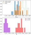 |
Fig. 1. Top: distributions of αBand for SGRBs (green) and for both LGRBs with and without the low-energy spectral break (orange and blue histogram). Bottom: distributions of α1,2SBPL and α2,2SBPL of the 12 LGRBs best fitted by the 2SBPL (i.e., with the low-energy spectral break). Distributions are normalized to their peak values. |
In the bottom panel of Fig. 1 we show the distributions of the indices α1,2SBPL (red) and α2,2SBPL (violet) for the 12 LGRBs best fitted by the 2SBPL (i.e., with an identified low-energy spectral break). The characteristic values (mean, median, and 1σ dispersion) of the distributions in Fig. 1 are reported in Tables 4 and 5.
From the comparison of the distributions shown in Fig. 1 we find that:
-
SGRBs (green dashed histogram) have a harder spectral slope αBand than LGRBs without a break (blue histogram). A Kolmogorov-Smirnov (KS) test11 among the two distributions returns a p-value of 0.004, rejecting the null hypothesis that these GRBs are drawn from the same underlying distribution. This is consistent with previous studies (Ghirlanda et al. 2004, 2009);
-
the value of αBand for LGRBs with a break (orange histogram in Fig. 1, top panel) is on average harder (see Table 4) than the value for LGRBs with no break (blue histogram). However, the two distributions are indistinguishable (a KS test between the orange and blue distributions has a chance probability p = 0.08);
-
the distributions of α1,2SBPL and α2,2SBPL (red and violet histograms in Fig. 1, bottom panel) are peaked at −0.71 and −1.71, not far from the typical values −2/3 and −3/2 expected for synchrotron spectrum from marginally fast cooling electrons;
-
LGRBs without a break have an αBand distribution that is slightly softer than α1,2SBPL but harder than α2,2SBPL (cf. the blue histogram in the top panel with the red and violet histogram in the bottom panel of Fig. 1 respectively). This might suggest that when the spectral data are not sufficient to constrain and identify a spectral break, the Band function returns a value of the low-energy index that is an average between the index α1,2SBPL and α2,2SBPL. This possibility is investigated with simulations in the following section;
-
the distribution of αBand of SGRBs (green) is similar to the α1,2SBPL distribution of LGRBs with a break: a KS test between the two returns p = 0.16. This suggests that the power-law segment α2,2SBPL separating Ebreak from Epeak is not present in SGRBs, i.e., Ebreak ∼ Epeak.
4. Origin of the value αBand ∼ −1
The spectral analysis presented in this paper confirms the presence of two classes of LGRBs: those requiring two power-law segments (α1,2SBPL and α2,2SBPL) to describe the spectrum at energies E < Epeak, and those for which this part of the spectrum is well described by a single power law (αBand). As the values of αBand are typically softer than α1,2SBPL but harder than α2,2SBPL, we investigate the possibility that spectra best fitted by Band are hiding a spectral break that is difficult to identify with a certain statistical significance due to the lack of enough signal at low energies, and/or to the proximity of Ebreak to Epeak, and/or to the proximity of Ebreak to the low-energy edge of the GBM sensitivity. If this is correct, we would expect to see a dependence of αBand on the values of Ebreak and Epeak and on their separation. Specifically, we expect that when the underlying spectrum has a break, the fit with the Band function will return a hard αBand ∼ α1,2SBPL when Ebreak ∼ Epeak, and, conversely, a soft αBand ∼ α2,2SBPL when Ebreak ≪ Epeak.
A strong correlation is not expected, as the value of αBand should depend not only on the ratio RE = Ebreak/Epeak, but also on the absolute value of Epeak (or, equivalently, Ebreak), and also on the specific values of α1,2SBPL and α2,2SBPL. To better investigate this effect and its presence in the spectra, we performed a set of simulations that are described in the following sections.
4.1. Band function response to a spectral break
In this first section we investigate how the presence of a spectral break generally affects the results of a fit performed using the Band function. We simulate GRB prompt spectra with input model 2SBPL, keeping fixed all the parameters and varying solely Ebreak. The adopted input parameters are α1,2SBPL = −0.65, α2,2SBPL = −1.67, Epeak = 1000 keV, β2SBPL = −2.5. These input values have been chosen in order to reproduce a typical LGRB of our sample (see the fit results in Sect. 3). For these simulations, we use the GBM background and response matrix files from one of the GRBs in our sample. We verified that choosing different background and response matrix files belonging to any other GRB in our sample does not affect the simulation results.
Each simulated spectrum is then fitted with the input model (a 2SBPL with parameters free to vary) and also with a Band function. For each value of Ebreak, we repeated the simulation 200 times, obtaining (for each parameter and for the reduced chi-square) a distribution of values. From these distributions we extracted the mean value and its 68% confidence interval. Figure 2 shows the parameters returned by the Band fits as a function of the position of the energy break. This exercise is repeated for two different cases, with a rather high average S/N12 (∼21, left-hand panel) and a S/N ratio that is approximately a factor 10 lower (∼2.7, right-hand panel). They represent simulated spectra of a GRB with a fluence of ∼3.5 ⋅ 10−4 erg cm−2 and ∼3.5 ⋅ 10−5 erg cm−2, respectively. The input parameters used for the 2SBPL function used for the simulations (α1,2SBPL, α2,2SBPL, Epeak, β2SBPL) are marked by dashed horizontal lines. We distinguish the best-fitting model according to our criterion based on the AIC (in Fig. 2, diamonds: 2SBPL, circles: Band).
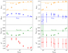 |
Fig. 2. Band function parameters as a function of the position of the energy break Ebreak of the 2SBPL function. Each plot shows the parameters of the Band function fitted to a series of spectra simulated assuming the 2SBPL function whose parameter values are marked by the horizontal dashed lines. Top: low-energy slope αBand (orange symbols) and high-energy slope βBand (blue symbols). Middle: energy peak Epeak, Band (green symbols). Bottom: fit |

The values of αBand obtained by fitting the simulated spectra with the Band function (orange symbols in the top panel) correlate with Ebreak: a low value of Ebreak makes αBand ≈ α2,2SBPL. On the other hand, as Ebreak increases (and approaches Epeak which in this example is 1 MeV) αBand ≈ α1,2SBPL. In between, the value of αBand is an average of α1,2SBPL and α2,2SBPL, depending on the position of Ebreak. Given the presence of only a single break in the Band function (i.e., Epeak, Band) the other parameters (βBand and Epeak, Band) also depend on the position of the break: βBand (blue symbols) always assumes softer values compared to the input one, unless Ebreak ∼ Epeak. Epeak, Band (green symbols) is an average of Ebreak and Epeak of the 2SBPL function and approaches the input value when Ebreak is very low or when Ebreak ∼ Epeak.
These results hold for both S/Ns. The main difference is in the uncertainties on the best fit parameters (larger for the case with lower S/N) and, most notably, on the behavior of the  . In the case with lower S/N, the
  of the Band fit is always acceptable (∼1), regardless of the value of Ebreak. This shows that, even though the input spectrum has a spectral break and this break falls within the GBM energy range, identification of the break is not possible in a spectrum with a relatively low S/N, and the best-fit model is a Band function. We note that a fluence of 3.5 ⋅ 10−5 erg cm−2 or less is representative of the majority of LGRBs detected by Fermi/GBM. If the S/N is increased by a factor of ten (left-hand panel), the
  of the fit with the Band function depends on Ebreak: only when the break is at the very-low-energy end of the GBM spectral range (Ebreak ≲ 10 keV) or close to Epeak (Ebreak ≳ 500 keV) does the fit with the Band function return an acceptable
  . Despite the high S/N, in such cases the break is hardly identifiable (ΔAIC < 6).
Finally, we notice that even when the Band function returns an adequate fit, (i.e., when Ebreak ≲ 10 keV or Ebreak ∼ Epeak) the resulting values of αBand, βBand, and Epeak, Band might largely deviate from the values of the input spectrum.
4.2. Spectral simulations: RE − αBand trend
In order to further investigate the RE − αBand trend, we focus first on the 12 LGRBs analyzed in this work that have a spectral break Ebreak. In Fig. 3 we show (orange symbols) their ratio RE = Ebreak/Epeak (from the fits of the 2SBPL) versus αBand (from the fit of the same spectrum with the Band function). LGRBs with a break are located in the range RE ∈ [0.04, 0.5] and, if their spectra are fitted with the Band function, the resulting αBand is in the range αBand ∈ [ − 1.1, −0.2]. A broad trend in the RE − αBand plane appears among the points. The Pearson correlation coefficient is 0.56 and the associated chance probability value p = 0.05.
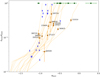 |
Fig. 3. 12 LGRBs best fitted by a 2SBPL (Table 1) shown with orange symbols. Their value of RE = Ebreak/Epeak is shown vs. the value of the index αBand that is obtained by fitting their spectrum with a Band function. SGRBs (whose spectrum is always best fitted by the Band function) are represented here assuming that, if the underlying spectrum were 2SBPL, it would be expected to have Ebreak ∼ Epeak (green symbols). The orange dashed lines show the results of simulations (see Sect. 4.2); blue arrows represent the upper and lower limits on RE for the 15 LGRBs whose spectra are best fitted by Band (see Sect. 4.3). |
For each of these GRBs, we simulate13 spectra with the 2SBPL function with parameter values fixed to the best-fit values (reported in Table 1) except for Ebreak, which we vary between 0.01Epeak and Epeak. For each GRB, we used the corresponding GBM background and response matrix files for the corresponding simulations. Simulated spectra were renormalized in order to maintain the energy-integrated flux of the real spectrum constant while moving Ebreak. Low values of RE place the break below the GBM low-energy threshold, i.e., 8 keV, in those GRBs with Epeak,2SBPL < 800 keV. We then refit the simulated spectra with the Band function and derive αBand. The simulation of each spectrum is repeated 200 times to build the distribution of αBand and estimate its mean value and 68% confidence interval.
In Fig. 3 we show, for each of the 12 LGRBs, the corresponding αBand returned by the fit with the Band function for each input value of RE (orange dashed line). These curves show that αBand depends on the relative position between break and peak energy, with small ratios resulting in soft spectra and large ratios resulting in harder spectra, as expected. These simulations show that the value of αBand is a “weighted” mean of the α1,2SBPL and α2,2SBPL slopes. Moreover, different curves show similar trends, showing that the different values of Epeak and input α1,2SBPL and α2,2SBPL are responsible for the dispersion in the plane. The dispersion of the curves is similar to the dispersion in the real data.
From the tracks of the orange dashed lines shown in Fig. 3 we can speculate that, when the best-fit model is a Band function, values of αBand harder than ∼ − 1.0 could be consistent with the presence of an Ebreak in the proximity (i.e., until one order of magnitude lower) of Epeak, while values softer than ∼ − 1.0 could indicate the presence of Ebreak far from (i.e., more than one order of magnitude lower than) Epeak. This possibility is investigated in the following section, through spectral simulations.
4.3. Spectral simulations: origin of the spectra without a low-energy break
Fifteen LGRBs in our sample do not show the presence of a low-energy spectral break. Through spectral simulations, we now propose to investigate whether or not it is still possible for these GRBs to have a low-energy break, even though the best-fit model is a simple Band function. The simulation now assumes that also in these 15 GRBs the spectrum has the shape of the 2SBPL function and infers constraints on its parameters by requiring that the fit with the Band function is not only acceptable but also preferred over a 2SBPL, and returns as best-fit values the same values as the real spectrum.
Based on the trend found between RE and αBand, we would expect that if the spectrum is intrinsically a 2SBPL and Ebreak lies at low energies, the Band function could adequately fit the simulated spectrum and result in αBand ∼ α2,2SBPL. Similarly, if the spectrum is intrinsically a 2SBPL and Ebreak lies close to Epeak, the Band function could return αBand ∼ α1,2SBPL. For each burst, the spectra simulated with the 2SBPL function maintain the same fluence of the real GRB.
We repeat the simulations for different values of the 2SBPL parameters. In particular:
-
α1,2SBPL is sampled uniformly within the range [ − 0.3, −1.05] with steps of 0.03;
-
α2,2SBPL is sampled uniformly in the interval ∈[−1.1, −1.9] with steps of 0.03;
-
Ebreak is sampled between 2 keV and the energy peak with steps of 2 keV;
-
β2SBPL is fixed to the value obtained from the fit with the Band function.
For each combination of parameters, we simulate ten spectra. We assume the background and response matrix files of each GRB for these simulations. These spectra are then refitted with both the 2SBPL and Band functions. From the built parameter distributions we derive the mean values and 68% confidence interval. Once we refit the spectrum with a Band function we accept the simulation if the Band fit satisfies the following conditions:
-
it is statistically equivalent to the fit with the 2SBPL, i.e., ΔAIC < 6;
-
its αBand and βBand are consistent, within 1σ, with the values inferred from the real spectrum;
-
its Epeak is consistent, within 3σ, with the value inferred from the real spectrum.
For each of the 15 LGRBs that do not explicitly show a break, we find a significant number of parameter combinations for which the 2SBPL functions were able to satisfactorily reproduce the real spectrum.
In particular, for all these LGRBs we are able to set either a plausible maximum or minimum value for Ebreak and constrain either α2,2SBPL or α1,2SBPL in an interval. These are represented with the blue arrows in Fig. 3. The limits for Ebreak and the low-energy slope intervals are listed in Tables 6 and 7.
Constraints on α2,2SBPL and maximum Ebreak (in keV) for GRBs with soft αBand that did not show an energy break in their time-integrated spectrum.
Constraints on α1,2SBPL and minimum Ebreak (in keV) for GRBs with hard αBand that did not show an energy break in their time-integrated spectrum.
5. Discussion and conclusions
The prompt emission spectra of long GRBs are often fitted with the Band function, two power laws smoothly joined at the νFν peak. The low-energy index (below the peak energy Epeak) αBand ∼ − 1 has been used as an argument against the interpretation of the prompt emission as synchrotron (see e.g., Preece et al. 1998; Frontera et al. 2000; Ghirlanda et al. 2002). Recently, different groups identified a break, Ebreak, at low energies below Epeak (Oganesyan et al. 2017, 2018, 2019; Ravasio et al. 2018, 2019) paving the way towards a solution to the long-standing issue on the nature of the prompt emission process (see e.g., Daigne 2011; Uhm & Zhang 2014; Bošnjak et al. 2009; Ghisellini & Celotti 1999; Rees & Mészáros 1994; Sari et al. 1996, 1998).
According to these latter works, the prompt emission spectra of the brightest GRBs can be described with three power laws (with indexes α1,2SBPL below Ebreak, α2,2SBPL between Ebreak and Epeak and β above it) smoothly joined at the two breaks, namely Ebreak and Epeak.
If the spectrum is a 2SBPL, our simulations described in Sect. 4.1 show that when Ebreak is close to Epeak or below the low-energy threshold (Emin) of the instrument, the Band function gives αBand ∼ α2,2SBPL and αBand ∼ α1,2SBPL, respectively. Values of αBand ∼ −1 correspond to Ebreak between Emin and Epeak. Through the spectral analysis of a sample of GRBs selected with different criteria, Burgess et al. (2020) find that, when Ebreak ≲ Epeak, the values of αBand are distributed approximately ∈[−1.7, −0.5]. We argue that, if the break is a common feature of GRB spectra, the value of αBand is a proxy of its position with respect to Epeak.
This hypothesis is verified through the spectral analysis of a sample of 27 long and 9 short GRBs selected from within the Fermi sample with large fluence and large Epeak (Sect. 2) in order to ease the search for Ebreak, if present. In 12 out of the 27 long GRBs, we find Ebreak (i.e., the 2SBPL fits the data better than Band). Through spectral simulations, using these events as templates, we find that if the break is moved within the range delimited by Epeak and Emin, the fit with Band results in a softer (if Ebreak departs from Epeak) or harder (if Ebreak approaches Epeak) low-energy index αBand (dashed orange lines in Fig. 3). At the extremes, the values of α1,2SBPL and α2,2SBPL are found. Indeed, none of the SGRBs analyzed have a break, but they all have a relatively hard αBand which we suggest corresponds to Ebreak lying close to Epeak. Through dedicated spectral simulations (Sect. 4.3) we show that the 15 LGRBs best fitted by the Band function only (i.e., apparently without a break) could instead have a break close to Epeak, corresponding to αBand > −1 (upward arrows in Fig. 3), or close to Emin if αBand < −1 (downward arrows in Fig. 3).
Our analysis suggests that the low-energy break could be a more common feature than is suggested by direct spectral analysis. Indeed, the identification of the break in the spectra of GRBs detected by Fermi or Swift, currently only possible for a limited number of events (shown in Fig. 4), is hampered by (1) the separation of Ebreak from Epeak and (2) the spectral signal-to-noise ratio. We show (right panel of Fig. 2) that a burst with a typical fluence (e.g., 5 ⋅ 10−6 erg cm−2 ) detected by Fermi/GBM can be fitted by Band even if it has an additional break. Taken together, these effects explain why we were not able to find Ebreak in approximately half of the selected GRBs but, through simulations, were able to set an upper or lower limit on its possible value.
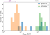 |
Fig. 4. Energy distribution of the spectral breaks identified in prompt spectra of GRBs, from the results of Oganesyan et al. (2018), Ravasio et al. (2019), and this work. The horizontal lines indicate the observational energy range of the instrumentation aboard THESEUS. |
With the currently available instruments, Swift and Fermi, it was possible to find Ebreak in a limited number of GRBs and with Ebreak at X-ray (∼few keV) and γ–ray (∼tens – hundreds keV) energies (Fig. 4). A few values of Ebreak between 10 and 100 keV are found.
Our results (Fig. 1 – bottom panel) show that the distributions of α1,2SBPL and α2,2SBPL are close to but slightly softer than the values predicted by synchrotron emission in the moderate fast cooling regime (Daigne 2011), that is, −3/2 and −2/3, respectively. This is partly thanks to our fits with the 2SBPL function rather than with the synchrotron model (see e.g., Burgess et al. 2015, 2020) and to the fact that we analyze time-integrated spectra to exploit the highest S/N in search of Ebreak. Time-resolved spectral analyses, indeed, often find harder spectral slopes (Nava et al. 2011a; Acuner & Ryde 2017) and, as shown by Ravasio et al. (2019), the distributions of α1,2SBPL and α2,2SBPL are closer to the typical synchrotron values.
With the Transient High-Energy Sky and Early Universe Surveyor (THESEUS) mission (Amati et al. 2018, 2021) proposed to ESA within the M5-class selection call, we expect that the spectral break will be detected in a larger fraction of events (Ghirlanda et al. 2021). The large effective area and the wide energy range covered by the two instruments on board THESEUS, namely the Soft X-ray Imager (SXI, 0.3–5 keV) and X-Gamma rays Imaging Spectrometer (XGIS, 2 keV–few MeV), will provide highly statistically significant prompt emission spectra from which Ebreak will be measured over a wider fluence range than is currently possible.
Accounting for the different redshift distributions, the peak energy of short and long GRBs become similar (Ghirlanda et al. 2015; Nava et al. 2012).
GRBs are classified into long and short based on the values of T90 reported in the Fermi online catalog, with a separation at 2 s.
A detailed analysis of the first peak (0−2.5 s) of GRB 130427A has been performed in Preece et al. (2014).
Through the error method built in XSPEC.
For all the statistical tests we have set the significance level at 0.05, i.e. we accept the null hypothesis if p > 0.05.
Calculated as  , where s and b are the source and background estimated counts, respectively (see e.g., Dereli-Bégué et al. 2020).
Spectral simulation performed within XSPEC with the fakeit tool.
Acknowledgments
G. O. acknowledges financial contribution from the agreement ASI-INAF n.2017-14-H.0. G. Ghirlanda acknowledges the Premiale project FIGARO 1.05.06.13 and INAF-PRIN 1.05.01.88.06.
References
- Acuner, Z., & Ryde, F. 2017, MNRAS, 475, 1708 [Google Scholar]
- Akaike, H. 1974, IEEE Trans. Autom. Control, 19, 716 [NASA ADS] [CrossRef] [MathSciNet] [Google Scholar]
- Amati, L., O’Brien, P., Götz, D., et al. 2018, Adv. Space Res., 62, 191 [Google Scholar]
- Amati, L., O’Brien, P. T., Götz, D., et al. 2021, Exp. Astron., submitted, [arXiv: 2104.09531] [Google Scholar]
- Band, D., Matteson, J., Ford, L., et al. 1993, ApJ, 413, 281 [NASA ADS] [CrossRef] [Google Scholar]
- Beniamini, P., & Piran, T. 2013, ApJ, 769, 69 [NASA ADS] [CrossRef] [Google Scholar]
- Bošnjak, Ž., Daigne, F., & Dubus, G. 2009, A&A, 498, 677 [NASA ADS] [CrossRef] [EDP Sciences] [Google Scholar]
- Burgess, J. M., Ryde, F., & Yu, H.-F. 2015, MNRAS, 451, 1511 [NASA ADS] [CrossRef] [Google Scholar]
- Burgess, J. M., Bégué, D., Greiner, J., et al. 2020, Nat. Astron., 4, 174 [NASA ADS] [CrossRef] [Google Scholar]
- Chand, V., Chattopadhyay, T., Oganesyan, G., et al. 2019, ApJ, 874, 70 [NASA ADS] [CrossRef] [Google Scholar]
- Daigne, F., Bošnjak, Ž., & Dubus, G. 2011, A&A, 526, A110 [NASA ADS] [CrossRef] [EDP Sciences] [Google Scholar]
- Dereli-Bégué, H., Pe’er, A., & Ryde, F. 2020, ApJ, 897, 145 [Google Scholar]
- Florou, I., Petropoulou, M., & Mastichiadis, A. 2021, MNRAS, 505, 1367 [Google Scholar]
- Frontera, F., Amati, L., Costa, E., et al. 2000, ApJS, 127, 59 [NASA ADS] [CrossRef] [Google Scholar]
- Frontera, F., Guidorzi, C., Montanari, E., et al. 2009, ApJS, 180, 192 [NASA ADS] [CrossRef] [Google Scholar]
- Geng, J.-J., Huang, Y.-F., Wu, X.-F., Zhang, B., & Zong, H.-S. 2018, ApJS, 234, 3 [NASA ADS] [CrossRef] [Google Scholar]
- Ghirlanda, G., Celotti, A., & Ghisellini, G. 2002, A&A, 393, 409 [NASA ADS] [CrossRef] [EDP Sciences] [Google Scholar]
- Ghirlanda, G., Ghisellini, G., & Celotti, A. 2004, A&A, 422, L55 [NASA ADS] [CrossRef] [EDP Sciences] [Google Scholar]
- Ghirlanda, G., Nava, L., Ghisellini, G., Celotti, A., & Firmani, C. 2009, A&A, 496, 585 [NASA ADS] [CrossRef] [EDP Sciences] [Google Scholar]
- Ghirlanda, G., Bernardini, M. G., Calderone, G., & D’Avanzo, P. 2015, J. High Energy Astrophys., 7, 81 [NASA ADS] [CrossRef] [Google Scholar]
- Ghirlanda, G., Salvaterra, R., Toffano, M., et al. 2021, Exp. Astron., in press, [arXiv:2104.10448] [Google Scholar]
- Ghisellini, G., & Celotti, A. 1999, ApJ, 511, L93 [NASA ADS] [CrossRef] [Google Scholar]
- Ghisellini, G., Ghirlanda, G., Oganesyan, G., et al. 2020, A&A, 636, A82 [CrossRef] [EDP Sciences] [Google Scholar]
- Goldstein, A., Burgess, J. M., Preece, R. D., et al. 2012, ApJS, 199, 19 [Google Scholar]
- Gruber, D., Goldstein, A., Weller von Ahlefeld, V., et al. 2014, ApJS, 211, 12 [NASA ADS] [CrossRef] [Google Scholar]
- Kaneko, Y., Preece, R. D., Briggs, M. S., Paciesas, W. S., & Meegan, C. 2006, ApJS, 166, 298 [NASA ADS] [CrossRef] [Google Scholar]
- Kouveliotou, C., Meegan, C. A., Fishman, G. J., et al. 1993, ApJ, 413, L101 [Google Scholar]
- Kumar, P., & McMahon, E. 2008, MNRAS, 384, 33 [NASA ADS] [CrossRef] [Google Scholar]
- Lien, A., Sakamoto, T., Barthelmy, S. D., et al. 2016, ApJ, 829, 7 [Google Scholar]
- Liu, R.-Y., & Wang, X.-Y. 2011, ApJ, 730, 1 [NASA ADS] [CrossRef] [Google Scholar]
- Meegan, C., Lichti, G., Bhat, P. N., et al. 2009, ApJ, 702, 791 [NASA ADS] [CrossRef] [Google Scholar]
- Nava, L., Ghirlanda, G., Ghisellini, G., & Celotti, A. 2011a, A&A, 530, A21 [NASA ADS] [CrossRef] [EDP Sciences] [Google Scholar]
- Nava, L., Ghirlanda, G., Ghisellini, G., & Celotti, A. 2011b, MNRAS, 415, 3153 [NASA ADS] [CrossRef] [Google Scholar]
- Nava, L., Salvaterra, R., Ghirlanda, G., et al. 2012, MNRAS, 421, 1256 [Google Scholar]
- Oganesyan, G., Nava, L., Ghirlanda, G., & Celotti, A. 2017, ApJ, 846, 137 [NASA ADS] [CrossRef] [Google Scholar]
- Oganesyan, G., Nava, L., Ghirlanda, G., & Celotti, A. 2018, A&A, 616, A138 [NASA ADS] [CrossRef] [EDP Sciences] [Google Scholar]
- Oganesyan, G., Nava, L., Ghirlanda, G., Melandri, A., & Celotti, A. 2019, A&A, 628, A59 [NASA ADS] [CrossRef] [EDP Sciences] [Google Scholar]
- Pe’er, A., Zhang, B.-B., Ryde, F., et al. 2012, MNRAS, 420, 468 [NASA ADS] [CrossRef] [Google Scholar]
- Preece, R. D., Briggs, M. S., Mallozzi, R. S., et al. 1998, ApJ, 506, L23 [NASA ADS] [CrossRef] [Google Scholar]
- Preece, R., Burgess, J. M., von Kienlin, A., et al. 2014, Science, 343, 51 [NASA ADS] [CrossRef] [Google Scholar]
- Ravasio, M. E., Oganesyan, G., Ghirlanda, G., et al. 2018, A&A, 613, A16 [NASA ADS] [CrossRef] [EDP Sciences] [Google Scholar]
- Ravasio, M. E., Ghirlanda, G., Nava, L., & Ghisellini, G. 2019, A&A, 625, A60 [NASA ADS] [CrossRef] [EDP Sciences] [Google Scholar]
- Rees, M. J., & Mészáros, P. 1994, ApJ, 430, L93 [NASA ADS] [CrossRef] [Google Scholar]
- Ronchi, M., Fumagalli, F., Ravasio, M. E., et al. 2020, A&A, 636, A55 [NASA ADS] [CrossRef] [EDP Sciences] [Google Scholar]
- Ryde, F., Axelsson, M., Zhang, B. B., et al. 2010, ApJ, 709, L172 [NASA ADS] [CrossRef] [Google Scholar]
- Sakamoto, T., Barthelmy, S. D., Baumgartner, W. H., et al. 2011, ApJS, 195, 2 [NASA ADS] [CrossRef] [Google Scholar]
- Sari, R., Narayan, R., & Piran, T. 1996, ApJ, 473, 204 [NASA ADS] [CrossRef] [Google Scholar]
- Sari, R., Piran, T., & Narayan, R. 1998, ApJ, 497, L17 [NASA ADS] [CrossRef] [Google Scholar]
- Uhm, Z. L., & Zhang, B. 2014, Nat. Phys., 10, 351 [NASA ADS] [CrossRef] [Google Scholar]
- von Kienlin, A., Meegan, C. A., Paciesas, W. S., et al. 2020, ApJ, 893, 46 [CrossRef] [Google Scholar]
- Yu, H.-F., Preece, R. D., Greiner, J., et al. 2016, A&A, 588, A135 [NASA ADS] [CrossRef] [EDP Sciences] [Google Scholar]
All Tables
Results of the fits performed using the Band function for the SGRBs in our sample.
Constraints on α2,2SBPL and maximum Ebreak (in keV) for GRBs with soft αBand that did not show an energy break in their time-integrated spectrum.
Constraints on α1,2SBPL and minimum Ebreak (in keV) for GRBs with hard αBand that did not show an energy break in their time-integrated spectrum.
All Figures
|
Fig. 1. Top: distributions of αBand for SGRBs (green) and for both LGRBs with and without the low-energy spectral break (orange and blue histogram). Bottom: distributions of α1,2SBPL and α2,2SBPL of the 12 LGRBs best fitted by the 2SBPL (i.e., with the low-energy spectral break). Distributions are normalized to their peak values. |
| In the text | |
|
Fig. 2. Band function parameters as a function of the position of the energy break Ebreak of the 2SBPL function. Each plot shows the parameters of the Band function fitted to a series of spectra simulated assuming the 2SBPL function whose parameter values are marked by the horizontal dashed lines. Top: low-energy slope αBand (orange symbols) and high-energy slope βBand (blue symbols). Middle: energy peak Epeak, Band (green symbols). Bottom: fit |
| In the text | |
|
Fig. 3. 12 LGRBs best fitted by a 2SBPL (Table 1) shown with orange symbols. Their value of RE = Ebreak/Epeak is shown vs. the value of the index αBand that is obtained by fitting their spectrum with a Band function. SGRBs (whose spectrum is always best fitted by the Band function) are represented here assuming that, if the underlying spectrum were 2SBPL, it would be expected to have Ebreak ∼ Epeak (green symbols). The orange dashed lines show the results of simulations (see Sect. 4.2); blue arrows represent the upper and lower limits on RE for the 15 LGRBs whose spectra are best fitted by Band (see Sect. 4.3). |
| In the text | |
|
Fig. 4. Energy distribution of the spectral breaks identified in prompt spectra of GRBs, from the results of Oganesyan et al. (2018), Ravasio et al. (2019), and this work. The horizontal lines indicate the observational energy range of the instrumentation aboard THESEUS. |
| In the text | |
Current usage metrics show cumulative count of Article Views (full-text article views including HTML views, PDF and ePub downloads, according to the available data) and Abstracts Views on Vision4Press platform.
Data correspond to usage on the plateform after 2015. The current usage metrics is available 48-96 hours after online publication and is updated daily on week days.
Initial download of the metrics may take a while.