| Issue |
A&A
Volume 652, August 2021
|
|
|---|---|---|
| Article Number | A108 | |
| Number of page(s) | 10 | |
| Section | Extragalactic astronomy | |
| DOI | https://doi.org/10.1051/0004-6361/202140797 | |
| Published online | 19 August 2021 | |
Fourcade-Figueroa galaxy: A clearly disrupted superthin edge-on galaxy⋆
1
Instituto Argentino de Radioastronomía, CONICET-CICPBA-UNLP, CC5 (1897) Villa Elisa, Prov. de Buenos Aires, Argentina
e-mail: This email address is being protected from spambots. You need JavaScript enabled to view it.
2
Facultad de Ciencias Astronómicas y Geofísicas, UNLP, Paseo del Bosque s/n, 1900 La Plata, Argentina
3
Ruhr University Bochum, Faculty of Physics and Astronomy, Astronomical Institute, 44780 Bochum, Germany
4
CSIRO Astronomy and Space Science, Australia Telescope National Facility, PO Box 76 Epping, NSW 1710, Australia
5
Western Sydney University, Locked Bag 1797, Penrith, NSW 2751, Australia
Received:
12
March
2021
Accepted:
4
June
2021
Abstract
Context. Studies of the stellar and the H I gas kinematics in dwarf and low surface brightness (LSB) galaxies are essential for deriving constraints on their dark matter distribution. Moreover, a key component to unveil in the evolution of LSBs is to determine why some of them can be classified as superthin.
Aims. We aim to investigate the nature of the proto-typical superthin galaxy Fourcade-Figueroa (FF) to understand the role played by the dark matter halo in forming its superthin shape and to investigate the mechanism that explains the observed disruption in the approaching side of the galaxy.
Methods. Combining new H I 21 cm observations obtained with the Giant Metrewave Radio Telescope with archival data from the Australia Telescope Compact Array we were able to obtain sensitive H I observations of the FF galaxy. These data were modelled with a 3D tilted ring model in order to derive the rotation curve and surface brightness density of the neutral hydrogen. We subsequently used this model, combined with a stellar profile from the literature, to derive the radial distribution of the dark matter in the FF galaxy. Additionally, we used a more direct measurement of the vertical H I gas distribution as a function of the galactocentric radius to determine the flaring of the gas disk.
Results. For the FF galaxy, the Navarro-Frenk-White dark matter distribution provides the best fit to the observed rotation curve. However, the differences with a pseudo-isothermal halo are small. Both models indicate that the core of the dark matter halo is compact. Even though the FF galaxy classifies as superthin, the gas thickness about the galactic centre exhibits a steep flaring of the gas that agrees with the edge of the stellar disk. In addition, FF is clearly disrupted towards its north-west side, clearly observed at optical and H I wavelengths. As suggested previously in the literature, the compact dark matter halo might be the main cause for the superthin structure of the stellar disk in FF. This idea is strengthened through the detection of the disruption; the fact that the galaxy is disturbed also appears to support the idea that it is not isolation that causes its superthin structure.
Key words: galaxies: groups: individual: ESO270-G017 / galaxies: interactions / radio lines: galaxies
The reduced ATCA+GMRT data cube (FITS file) are only available at the CDS via anonymous ftp to cdsarc.u-strasbg.fr (130.79.128.5) or via http://cdsarc.u-strasbg.fr/viz-bin/cat/J/A+A/652/A108
© ESO 2021
1. Introduction
In 1993, Karachentsev, Karachentseva and Parnovskij published the Flat Galaxy Catalogue (FGC, Karachentsev et al. 1993). A revised version of it was released in 1999 (RFGC, Karachentsev et al. 1999). The catalogue contains disk-like edge-on galaxies with a major-to-minor stellar axis ratio a/b > 7. Superthin galaxies are a special type of flat galaxies with a/b ≳ 10. These are gas-rich low surface brightness (LSB) galaxies, with little or no obvious bulge component, minimal dust absorption (Matthews & Wood 2001), blue optical colours (Dalcanton & Bernstein 2000), low metallicities (Roennback & Bergvall 1995), low current star formation, and a high ratio of dynamic to H I mass (de Blok & Bosma 2002). These characteristics suggest that these galaxies are some of the least evolved galaxies in the Universe. In addition, their high inclinations and simple structure allow us to study the effects produced by internal as well as external processes (Uson & Matthews 2003). All theses characteristics make the superthin galaxies an ideal laboratory to for investigating the early stages of disk galaxy evolution.
The cosmological paradigm of hierarchical galaxy formation and evolution proposes that galaxies are subject to merging and interaction. Thus, the disk structure and thickness in galaxies are affected by the environment (Toth & Ostriker 1992; Odewahn 1994; Reshetnikov & Combes 1997; Schwarzkopf & Dettmar 2001). This suggests that flat-disk galaxy must remain isolated to persist as a superthin. However, some of these galaxies are found in groups of galaxies as well as in the field (Kautsch 2009). Therefore the question arises how the pure disk survives? A possible explanation is the presence of a massive dark matter (DM) halo that stabilises their disks against perturbations (Zasov et al. 1991; Gerritsen & de Blok 1999); moreover, Mosenkov et al. (2010) found a correlation between the thickness of stellar disks and relative mass of the DM halo. Banerjee & Jog (2013) showed that the determination of the superthin disk distribution in low-luminosity bulge-less galaxies is ruled by the compactness of the DM. This idea is supported by the studies of four superthin and proto-typical superthin galaxies UGC 7321 (O’Brien et al. 2010; Banerjee & Bapat 2017), IC 2233, IC 5249 (Banerjee & Bapat 2017), and FGC 1540 (Kurapati et al. 2018). As this sample is still extremely small, any single addition to it can still provide significant new insights or strengthen the current ideas about the nature of superthin galaxies.
Studies of the stellar and the H I gas kinematics in dwarf and LSB galaxies are essential for deriving constraints on the DM distribution (Rubin et al. 1978; McGaugh & de Blok 1998; Banerjee et al. 2010). Moreover, understanding why some LSBs are superthin can contribute to the overall understanding of LSBs and DM in general. In this paper we focus on the prototypical superthin Fourcade-Figueroa (FF) galaxy. By combining new Giant Metrewave Radio Telescope (GMRT) data with archival Australia Telescope Compact Array (ATCA) data, we obtained a high-resolution sensitive H I observation of the galaxy. After modelling the gas distribution, we use the derived rotation curve to determine the DM distribution in the FF galaxy.
The FF galaxy, also known as ESO 270−G017, was discovered in 1970 (Fourcade 1970) as an elongated and diffuse object, see Fig. 1, located approximately at 2° 32′ south-east of the core of the radio galaxy Centaurus A (Cen A; NGC 5128). The galaxy was initially thought to be part of the Centaurus A group (Colomb et al. 1984; Tully et al. 2013; Karachentsev & Kudrya 2014). However, recent distance estimates place it just beyond Centaurus A at a distance of 7 Mpc (Karachentsev et al. 2015). Karachentsev et al. (1999) reported a stellar axial ratio of a/b = 9.1 (or b/a = 0.1). The ratio b/a is a strong parameter to determine the flatness of a galaxy because typical b/a measurements of flat galaxies (between 0.04 to 0.14, Karachentsev et al. 1999) are quite different from the usual values found in the literature regarding all types. The major and minor axes can also be used to derive the galaxy inclination i as a first approximation, as cos(i) = b/a.
 |
Fig. 1. FF three-colour image composites from the B, V, and I bands published by Ho et al. (2011). |
We list the main optical properties of the FF galaxy in Table 1. From WISE observations, Wang et al. (2017) obtained the two-dimensional structural surface brightness decomposition of FF. This profile has a scale length of 4.4 kpc. From their cleaned 3.4 μm WISE image, we determine an inner (r < 2.8 kpc) scale height of 0.47 kpc. This results in a ratio hr/hz ∼ 9.4, again confirming that the FF galaxy can be considered a superthin galaxy (see also Kregel et al. 2002). FF is a good candidate on which to perform mass-modelling and thereby determine its DM halo. Despite its superthin structure, the FF galaxy shows an asymmetry towards its north-west side (Fourcade 1970), like a shred or disruption, which is observed in both optical and H I images. The origin of this disruption remains unclear.
Optical properties of the Fourcade-Figueroa galaxy.
The paper is organised as follows: in Sect. 2 we describe the observations and data reduction, including the combination process between data sets from very different radio interferometers; in Sect. 3 we present the H I distribution and kinematics; in Sect. 4 we describe the mass models; in Sect. 5 we present the mass-modelling results and the discussion; in Sect. 6 we present the shred and in Sect. 7 the summary.
2. HI Observations and data reduction
The FF galaxy has been observed at 1420 MHz with the Australia Telescope Compact Array (ATCA). The data were downloaded from the Australia Telescope Online Archive (ATOA1). The data were published by Koribalski et al. (2018) and are part of the Local Volume H I Survey (LVHIS) project. Notwithstanding the existence of previous observations, new ones were carried out at the same frequency with the GMRT, which provides a better angular and velocity resolution. Additionally, it has better coverage of the uv-plane, which can be further improved upon by using observations from both telescopes. In the following subsections we describe the observations and data calibration for both ATCA and GMRT as well as the combination process.
2.1. Australia Telescope Compact Array data
The ATCA 21cm observations were carried out in January 1993, June and July 1993, as well as November 2008 using the 750, 6A, and EW367 array configurations, respectively. The total integration time on-source was 27 h 40 min. The 8 MHz bandwidth divided into 512 channels resulted in a spectral resolution of 15.6 kHz, equivalent to ∼4 km s−1 per channel. A flux calibrator was observed at the beginning and end of each observing run for 10 min, ad a phase calibrator was observed between the target scans every 45 min; see Table 2 for more details.
ATCA and GMRT observing parameters.
Data reduction and analysis were performed with the MIRIAD software (Sault et al. 1995) using standard procedures. We calibrated each data set separately, using PKS 0407–658 (750/6A array) and PKS 1934–638 (EW367 array) as primary flux and bandpass calibrators. PKS 1320–446 (750/6A array) and PKS 1421–490 (EW367 array) served as the phase calibrators. We used the MIRIAD task UVLIN to subtract the continuum. With a bandwidth of 8 MHz (see Table 2), we were able to select the line-free channels on either side of the detected H I emission.
2.2. Giant Metrewave Radio Telescope data
We observed the FF galaxy with the GMRT at 21cm for a total time of ∼14 h (project 28_069, PI P. Benaglia). The observations were carried out during June-July 2015 and January 2016 in the spectral zoom mode with the GMRT-Software backend. We used a 4.16 MHz bandwidth with 512 channels, which results in a spectral resolution of 8.13 kHz, equivalent to 1.7 km s−1 per channel. The flux calibrator 3C 286 was observed at the beginning and end of the run. The source 1323–448 was used as the phase calibrator and was observed between the target scans; see Table 2 for more details.
The data were flagged and calibrated using the FLAGCAL pipeline (Prasad & Chengalur 2011). In addition, we extensively used for further analysis, visualisation and multi-wavelength imaging the MIRIAD software package and kvis, part of the karma package (Gooch 1996). To check the calibration process, all the calibrator sources were imaged. GMRT does not do online Doppler tracking. Thus, the Astronomical Imaging Processing System (AIPS, Greisen 2003) task CVEL was implemented to apply the Doppler shift corrections. All the data sets were combined using the AIPS task DBCON. The continuum subtraction was made with MIRIAD task UVLIN; we were able to select the line-free channels on either side of the detected H I emission.
2.3. Combining ATCA and GMRT radio interferometer data
The benefits of complementing the GMRT with ATCA data are the improvement of the signal-to-noise ratio by ∼15%, a better uv plane coverage that should improve the quality of the final images, and a better angular resolution. In this manner, we will get the most out of observations; we can map the extended structures with excellent angular resolution.
As the GMRT is a non-coplanar array, we should in principle should account for this when imaging the data, that is, a w-projection is required. However, for our current observations, we estimated that the shift introduced by ignoring this effect would lead to a shift of 2.25″ at the first null of the primary beam over a 12h observation. This leads to a 10% error on the synthesised beam if we limit our baselines to be < 28 kλ. As MIRIAD is the only package that allows us to combine the data in he uv-domain while taking into account the primary beam correction, we chose to image the data without a w-projection. As for both observations the band width was too narrow to perform a self-calibration, we conclude that this problem will not affect the image cubes if we just use the visibilities up to 28 kλ (equivalent to 6 km).
We carried out the data combination in the uv domain using the MIRIAD software. Both data sets need to have the same velocity system reference and channel increment organised in the same way; the tasks CVEL, SPLIT and BLOAT from AIPS were used to arrange the visibilities of the different observations on the same frequency grid. We implemented the MIRIAD routine INVERT to perform a linear mosaic of these 21 cm GMRT and ATCA data. The INVERT task optimises the signal-to-noise ratio using the system temperature. For this, after we loaded the GMRT data sets into MIRIAD, we had to add the value of the system temperature in the header. This parameter was gathered from the GMRT user’s manual2. The deconvolution process was carried out using the maximum entropy deconvolution, MOSMEM task, for a mosaiced image. The final synthesised beam was created with the task MOSSPSF and applied during restoration.
To summarise, the final H I cube was made using baselines up to 28 kλ and natural weighting. The synthesised beam is 20″ × 20″, which results in a physical resolution of 673 pc × 673 pc at the adopted FF distance. The corresponding r.m.s. noise is 2 mJy beam−1.
3. HI distribution and kinematics
To ensure that our combined data set was free from systematic biases, we first extracted the line spectrum and compared it to the individual datasets and an archival single-dish observation. The results are shown in Fig. 2. The total line flux obtained from the combination data cube is FHI = 197 ± 0.4 Jy km s−1, which agrees with the value in the H I Parkes All-Sky Survey (HIPASS), FHI = 199.4 ± 15.1 Jy km s−1 (Koribalski et al. 2004), and LVHIS (Koribalski et al. 2018) with the LVHIS FHI = 224.7 Jy km s−1.
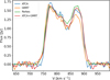 |
Fig. 2. Comparison of the FF global H I profile obtained using ATCA (light blue), GMRT (orange), Parkes (green, Koribalski et al. 2004), and the combination of ATCA and GMRT data (red). |
The global H I profile of the FF galaxy is shown in Fig. 2. For the profile derived from the combined cube (ATCA+GMRT data), the flux along the velocity axis remains mostly equal to or below that derived from Parkes data alone, as expected.
The H I diameter is DHI = 20′. The H I emission was detected from ∼720 to 920 km s−1. At a distance of 6.95 Mpc, this corresponds to a total H I mass of MHI = 2.2 × 10⁹ M⊙, which means that MHI/LB = 1.04. The systemic velocity of FF is 828 km s−1. The profile widths of 20% and 50% levels are 142 km s−1 and 120 km s−1.
3.1. H I distribution
Figure 3 shows the channels where the FF galaxy contains detectable H I emission. A visible disruption is observed in the channels covering the velocity ranges from 770 to 810 km s−1. The shred (Fourcade 1970; Thomson 1992) is clearly seen as a disruption in the distribution as well as the kinematics of the gas, and corresponds to the shred as seen in the optical. The disruption is at a projected radial distance ∼5 kpc from the centre, at the same position in which the H I distribution bends away from the major axis to the north, see Fig. 4. The H I is distributed over a diameter of ∼20′, almost twice the optical diameter (∼11.3′), see Fig. 4 top panels. The velocity field of FF is not regular, as shown in the bottom left panel in Fig. 4. The velocity dispersion varies between 5 and 15 km s−1, see the bottom right panel in Fig. 4. Because we study a (nearly) edge-on galaxy, the measured dispersion indicates the spread in coherent rotation along any line of sight, rather than a physical gas velocity dispersion.
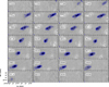 |
Fig. 3. ATCA+GMRT high-resolution H I channel maps of the Fourcade-Figueroa galaxy. The channel velocity is shown in the top left corner (in km s−1) and the synthesised beam (20″) in the bottom left corner of each panel. The contour levels are −6, 6, 15, 25, and 35 mJy beam−1. |
3.2. Vertical gas thickness
Considering the H I gas distribution in FF is asymmetric, we derived the thickness of the H I disk as a function of the galactocentric radius. The method we implemented follows the procedures laid out in Olling (1995) and O’Brien et al. (2010). The vertical H I profile of FF exhibits a high degree of asymmetry of the gas thickness about the galactic centre. At the receding side of the galaxy, the H I flares from a full width half maximum (FWHM) of 2.5 kpc at 5 kpc out to 3.5 kpc at 18 kpc. The steep flaring of the gas agrees with the edge of the stellar disk. Between 5 kpc and 15 kpc, the H I thickness seems to remain constant, except for a bump at 8 kpc. At the approaching side, the vertical H I thickness shows an irregular flaring profile. From 3 kpc to 5 kpc, the H I thickness is roughly constant with an FWHM of about 2 kpc. In the range between 5 kpc to 10 kpc, the H I gas flare from 2.3 kpc to 3.6 kpc, which agrees with the location of the shred. The steep gas flare at the mentioned galactocentric distance is coincident with the radius at which the stellar disk becomes fainter. Additionally, the line width of the velocity profiles (see Fig. 4) highly increases at this position. After 10 kpc (galactocentric radius), the H I disk thickness decreases at radii outside of 15 kpc; this agrees with the decrease in H I velocity dispersion. The linear size of the beam is ∼700 pc, and Fig. 5 shows that variations in vertical gas thickness occur on a much larger scale (a few kiloparsec, thus including several beams), and therefore override or at least minimise beam-smearing problems. On average, z0 is 32.6″ ± 0.2″or z0 = 1.1 ± 0.4 kpc at the assumed distance of 6.95 Mpc.
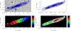 |
Fig. 4. ATCA+GMRT H I moment maps of the Fourcade-Figueroa galaxy. Top left panel: H I distribution overlaid on the DSS2 I-band image. The H I contour levels are 0.24, 0.9, 1.7, and 2.1 Jy beam−1 km s−1. Top right panel: H I distribution (same contours). Bottom left panel: velocity field, the contour levels are 768, 788, 808, 828, 848, 868, and 888 km s−1. Bottom right panel: velocity dispersion; the contour levels are 3, 8, 10, 12, and 15 km s−1. The H I distribution maps were made using the low-resolution cube with a synthesised beam of 20″ × 20″. |
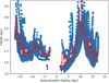 |
Fig. 5. Measured H I FWHM thickness (negative radius is receding). |
3.3. H I kinematics, 3D modelling and the rotation curve using FAT and TiRiFiC
The rotation curve was derived using the fully automatic TiRiFiC code (FAT, Kamphuis et al. 2015), which is a wrapper code around the tilted ring fitting code (TiRiFiC, Józsa et al. 2012), to perform a 3D modelling, and the source finder application (SoFiA, Serra et al. 2015) to estimate the initial parameters. We found that FAT is not capable of dealing with the varying noise statistics that are due to the primary beam correction. The final FAT model did not cover the full extent of the H I disk. Therefore the outer parts of the galaxy were fitted manually with TiRiFiC itself. Performing a 3D modelling by fitting the 3D observations directly as TiRiFiC and FAT routines do guarantees that problems such as beam smearing and projection effects are overcome, according to Józsa et al. (2012) and Kamphuis et al. (2015). Because the FF galaxy is clearly warped and asymmetric, we created a two-disk model in which each disk represents one half of the galaxy. The inclination was the most problematic parameter to fit; we attempted values between 80 and 90 degrees, and after the visual inspection of the results, we decided to fix it at 87 deg. From the vertical H I distribution analysis, we obtained that z0 is 1.1 ± 0.4 kpc on average. We therefore decided to fix this value in the model as well. To check the validity of the fits, visual comparisons between the data and models were performed in many different representations of the cubes, such as channel map by channel map, the velocity field, and the position velocity (pv) diagram parallel to the minor and major axis. For the error bars on the final rotation curve, we used the difference between the approaching and receding side; a minimum realistic error of 2 km s−1 was considered. Figure 6 shows that the rotation curve rises steeply in the innermost 4 kpc, then continues to rise slowly until the outermost radius. The maximum rotation speed is ∼72 km s−1. The de-projected H I radial surface brightness profile derived by FAT shows the H I surface density peak at ΣHI ∼ 5 M⊙ pc−2 in the centre but is mostly constant around ∼5, M⊙ pc−2 (see Fig. 6). The pv-diagram is shown in Fig. 7.
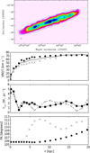 |
Fig. 6. First row: comparison of data (green) and model (blue) moment-zero maps. Rows 2–4: model parameters as a function of radius. The crosses and squares represent the approaching and receding halves of the FF galaxy. Second row: rotation curve. The solid curve corresponds to the mean rotation curve. Third row: de-projected H I gas surface distribution. Fourth row: position angle variation. |
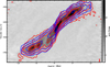 |
Fig. 7. H Ipv diagram along the major axis is shown in grey and red contours. The blue contour levels represent the pv of the model galaxy. The contour levels are 4, 9, 17, 29 and 39 mJy beam−1 km s−1. |
4. Mass models
4.1. Visible matter contribution
The rotation velocities due to the gravitational potentials of the stellar and gaseous disks were determined separately using the task ROTMOD of the Groningen Image Processing System (GIPSY, van der Hulst et al. 1992). Because the old stellar population dominates the total stellar mass in late-type galaxies and mid-infrared emission is less susceptible to dust extinction and is also not affected by recent star formation, the stellar contribution (V*) was derived using the stellar mass profile obtained by Wang et al. (2017) from WISE 3.4 μm infrared images. We assumed the vertical distribution as
where z0 is the disk scale-height (z0 = 0.47 kpc), see for instance van der Kruit & Searle (1981a,b). The gaseous contribution (Vgas) was derived using the de-projected H I radial surface density profile as derived by FAT and TiRiFiC. We considered a vertical density distribution given by the exponential law
where the value of z0 = 1.1 ± 0.4 kpc (see Sect. 3.2). The H I gas surface density distribution was then multiplied by a factor of 1.4 to account for the primordial helium, but we did not consider the presence of molecular H2 in our models. For late-type LSB spiral galaxies the ratio H2/HI is 10−3 (Matthews et al. 2005).
4.2. Dark matter Halo
We used the so-called pseudo-isothermal halo (ISO) and the Navarro, Frenk & White (NFW) density profiles to model the DM halo of the FF galaxy. The simplest model for a DM halo density profile is the pseudo-isothermal halo (Begeman et al. 1991). Its density profile is given by
![Mathematical equation: $$ \begin{aligned} V_{\rm ISO}(R) = V_{\rm inf} \sqrt{4\phi G \rho _0 (R_C)^2 \left[1-\left[\frac{R_c}{R}\arctan \left( \frac{R}{R_c}\right)\right]\right]}, \end{aligned} $$](/articles/aa/full_html/2021/08/aa40797-21/aa40797-21-eq4.gif)
where ρ0 is the central core density and Rc is the core radius of the halo. The rotational velocity expression at any radius R, due to an ISO DM halo, is VISO, and the asymptotic velocity of the halo is Vinf. Based on numerical simulations of DM halos, Navarro, Frenk & White (Navarro et al. 1996) described the radial density profile with the expressions:
Here Rs is the characteristic radius of the halo, ρcrit is the critical density of the universe, c =  is the concentration parameter and x =
  . R200 is the radius at which the average density of the NFW halo is 200ρcrit. R200 is in kpc and V200 = 0.73R200 is the rotation velocity at R200 in km s−1.
Theoretically, because the FF galaxy contains no bulge, the net rotation velocity V at a radius R is obtained by adding in quadrature the rotational velocity due to the gravitational potential of the stars, gas, and DM components,

here Υ* is the stellar mass-to-light ratio.
We made use of ROTMAS, a task in GIPSY (van der Hulst et al. 1992) that allows interactive modelling of rotation curves, with options for the addition of DM halo contribution. We carried out the disk-halo decomposition using different assumptions of it: a maximum disk, a minimum disk with gas, and a minimum disk.
5. Mass modelling: Results and discussion
As we described, the rotation curve fitting procedure typically has as free parameters the scale-length, the halo density, and the mass-to-light ratio of the stellar component. The last value is not known a priory. Its estimation is difficult and may differ from galaxy to galaxy. Cluver et al. (2014) obtained an empirical relation of the between mid-infrared emission of galactic disks and stellar mass-to-light ratios in the W1 and W2 WISE bands. Using this relation with the FF WISE photometric measurements available in Wang et al. (2017), we found that Υ⋆ = 0.8.
As the approaching side of the galaxy is clearly kinetically disturbed, we performed the mass-modelling only considering the rotation curve derived from the receding half of the FF galaxy.
5.1. Maximum disk
In the maximum disk model, the stellar disk is scaled to the maximum possible value, dominating the underlying gravitational potential (van Albada et al. 1985). Thus, it returns an upper limit to the Υ⋆ value and a lower bound on the DM distribution in the galaxy. The maximum disk model can be constructed in two different ways. First, by fixing Υ⋆ to a maximum possible value. For FF, we fixed it to 0.8. Second, by arbitrarily fixing Υ⋆ to the value that corresponds to the ∼75% contribution to the peak of the rotation curve at R = 2.2rs (Sackett 1997). In Fig. 8 we show the rotation curve decomposition with the maximum disk model constructed considering both methods, and in Table 3 we list the results. The values of the mass-to-light ratio Υ⋆ obtained for the best-fitting models considering the ∼75% contribution to the peak of the rotation curve at R = 2.2rs are an order of magnitude higher than the value derived considering the stellar population. Both ISO and the NFW halo give higher values of reduced χ2 of all the fits. Previous studies of LSBs and some superthin galaxies indicate that most galaxies of this type do not have a maximum disk (de Blok et al. 2008; Banerjee & Bapat 2017), because the structure in the stellar disk is not seen in the rotation curve.
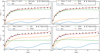 |
Fig. 8. Modelling the H I rotation curve of the Fourcade-Figueroa galaxy. Upper panels: ISO and the NFW halo based mass model for the maximum disk with Υ⋆ = 0.8. Lower panels: ISO and the NFW halo based mass model for the maximum disk considering ∼75% contribution to the peak of the rotation curve at R = 2.2rs. The orange line indicates the rotation curve due to the stellar disk, the blue line that due to the gas disk, the green line that due to the DM halo, and the red line shows the best-fitting model rotation curve. |
Results of the mass modelling of the FF galaxy for ISO and NFW DM halo profiles.
5.2. Minimum disk
The minimum disk model assumes that the rotation curve is entirely due to the presence of DM and therefore sets an upper bound on the DM density. We constructed two different minimum disk models: first, a minimum disk with gas. This model only considers the contribution of neutral hydrogen and helium to the rotation curve. In the upper panels of Fig. 9 we show the rotation curve decomposition with the minimum disk + gas, and in Table 3 we list the results. Second, a minimum disk in which the stellar and gas disk contributions are zero. In the lower panels of Fig. 9 we show the rotation curve decomposition with the minimum disk.
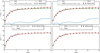 |
Fig. 9. Modelling the H I rotation curve of the Fourcade-Figueroa galaxy. Upper panels: ISO and the NFW halo based mass model for the minimum disk + gas. Lower panels: ISO and the NFW halo based mass model for the FF galaxy for the minimum disk. The orange line indicates the rotation curve due to the stellar disk, the blue line that due to the gas disk, the green line that due to the DM halo, and red shows the best-fitting model rotation curve. |
We present the mass modelling of the FF galaxy, carried out using ISO and NFW DM density profiles. The results are listed in Table 3. The best reduced χ2 values were obtained with the minimumdisk, especially the value obtained with the NFW DM halo. Thus, the contribution of the visible matter to the net gravitational potential is negligible. This result agrees with the trend observed in LSB and other superthin galaxies (de Blok et al. 2008; Banerjee & Bapat 2017; Kurapati et al. 2018). The ratio of the core radius of the halo and the scale length of the optical disk (RC/RD) is always lower than two for the ISO DM halo. This indicates that the core of the ISO halo is compact. Consequently, the DM halo dominates at the inner radii as well. Banerjee & Bapat (2017) obtained similar results for three superthin galaxies (UGC 7321, IC 5249 and IC 2233) as well as Kurapati et al. (2018) (FGC 1540). The compactness of the DM halo may cause the superthin disk distribution (Banerjee & Jog 2013).
5.3. Mass-modelling with MOND formalism
The modified newtonian dynamics (MOND) postulates that Newtonian dynamics breaks down at low acceleration (Milgrom 1983). This formalism rules out the presence of DM and takes into account the self-gravity of the stars and gas in galactic dynamics studies. There are two free parameters: the stellar mass-to-light ratio (Υ⋆), and the acceleration per unit length (a0).
In Fig. 10 we show the best-fitting rotation curve for the MOND formalism. In order to achieve a physically realistic value of a0, Υ⋆ was fixed to 0.8. The acceleration parameter resulted in a0 = 2694 ± 520 km2 s−1 kpc−1. The reduced χ2 is 42. This means that in the case of FF, the centrally concentrated mass indicated by the RC is not seen in the gas and stellar distribution. This in turn means there should be a very concentrated unseen baryonic component for MOND to work.
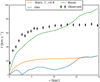 |
Fig. 10. Modelling H I rotation curve of the Fourcade-Figueroa galaxy using MOND. The orange line indicates the rotation curve due to the stellar disk, the blue line the rotation curve due to the gas disk, and the green line is the MOND best-fitting model rotation curve. |
6. Shred
Despite its superthin structure, the FF galaxy shows an asymmetry towards its north-west side, clearly observed in optical and H I moment maps. A series of features appears at the approaching side of the galaxy: First, the iso-velocity contours start to exhibit distortions only a few kiloparsec away from the centre, and at the location of the kinematic anomalies, we can also see a thickening of the emission that is observed in the integrated moment map. However, because of the edge-on orientation of the galaxy, a more sophisticated analysis is required to determine at which radial location this occurs. Second, the H I gas steeply flares as the stellar component becomes fainter. This is indicative of a change in mass in the disk (Sancisi & Allen 1979; Olling 1995). Additionally, at the same location, the dispersion velocity is higher.
The de-projected H I peak surface density is ΣHI ∼ 5 M⊙ pc−2, which is close to the mean value proposed by Cayatte et al. (1994) for Sbc galaxies (∼6 M⊙ pc−2). This value also agrees with the results found by Kurapati et al. (2018) and Banerjee & Bapat (2017) for similar superthin galaxies. Furthermore, in most of the gas disk of FF, the gas surface density seems to lie below that required for efficient star formation (Kennicutt 1989), and moreover, the overall density profile value is half of the peak surface density, see Fig. 6. Although the galaxy is forming some stars, this result is consistent with the very low star formation rate derived from optical observations (log(SFR) = −1.0 M⊙ yr−1) and the low radio continuum emission reported previously (Saponara et al. 2012); The evidence suggests that intense star formation activity is not the main cause of the observed disruption.
In 1992 Thomson (1992) proposed after the analysis of numerical simulations that the FF shred might arise because the FF galaxy undergoes a strong prograde interaction with the massive galaxy Cen A. This theory is currently ruled out. A recent more accurate distance estimate places FF just beyond Cen A (∼7 Mpc, Karachentsev et al. 2015). Another possible explanation of the observed vertical thickness is the interaction with a companion dwarf galaxy, which enhances star formation in a small region in the western-most part of the disk, generating this and the higher dispersion observed. The available UV images from GALEX3, although they partially cover the galaxy, provide an indication of this. Although the field of view is mostly filled with the galaxy, we visually searched for H I low-mass companions of the FF galaxy, but no recognisable companions were observed. However, Cen A appears to have an overabundance of the faintest dwarfs in comparison to its simulated analogues (Müller et al. 2019), indicating that interactions are likely, and the scenario of a dwarf galaxy accreted like the Sag dSph by the Milky Way turns very probable (Ruiz-Lara et al. 2020). This would be in contrast to superthin galaxies evolving in isolation. FF might be disturbed in such a way that it is evolving away from being a superthin galaxy, although the quiescent and thin approaching side appear to counter this idea. Most studies of superthin galaxies have so far presented this class as isolated objects, that is, devoid of interactions. An exception might be galaxy IC 2233, for which the authors explored the possibility of interaction with smaller nearby galaxies (Uson & Matthews 2003). That interactions do not destroy the superthin disks in these galaxies fits previous results (O’Brien et al. 2010; Banerjee & Bapat 2017; Kurapati et al. 2018), indicating that the compact DM halo is the main cause for the superthin structure of the stellar disk, not isolation.
7. Summary
We used the rotation curve, the H I surface density profile, and with the stellar profile obtained from the literature to construct mass models for the FF galaxy. The FF rotation curve, as well as its de-projected H I surface density profile, were derived by fitting a detailed 3D tilted ring model to the data. After assuming the ISO as well as a NFW DM halo, we found that both halos fit the observed rotation curve well, but the best reduced χ2 values were obtained with the minimum disk model considering an NFW halo. The results obtained from the mass modelling imply that the DM halo is compact. We derived the thickness of the H I disk as a function of the galactocentric radius. At the approaching side of the galaxy, the vertical H I thickness shows an irregular profile. The FF galaxy shows an asymmetry towards its north-west side, which is clearly observed in optical and H I images. The new distance establishes FF away from Cen A, which dismisses the hypothesis of past interaction between them. Even though we did not find H I low-mass companions for FF in our H I cubes, tidal interaction cannot be ruled out. Thus, the compact DM halo might be the main responsible for the superthin structure observed in the galaxy, not isolation.
Acknowledgments
J. S. is grateful to Arunima Banerjee for use full discussions and to Jing Wang for the mass profile. This paper is based on observations obtained with the Australia Telescope Compact Array (ATCA) and the Giant Metrewave Radio Telescope (GMRT). ATCA is part of the Australia Telescope National Facility (ATNF) which is funded by the Australian Government for operation as a National Facility managed by CSIRO. We acknowledge the Gomeroi people as the traditional owners of the Observatory site. GMRT is operated by the National Centre for Radio Astrophysics of the Tata Institute of Fundamental Research. We thank the staff of both radio telescopes who made these observations possible. This research has made use of the NASA/IPAC extragalactic database (NED) that is operated by the Jet Propulsion Laboratory, California Institute of Technology, under contract with the National Aeronautics and Space Administration. This work was partially supported by FCAG-UNLP, and ANPCyT project PICT 2017-0773. P. K. is partially supported by the BMBF project 05A17PC2 for D-MeerKAT.
References
- Banerjee, A., & Bapat, D. 2017, MNRAS, 466, 3753 [CrossRef] [Google Scholar]
- Banerjee, A., & Jog, C. J. 2013, MNRAS, 431, 582 [NASA ADS] [CrossRef] [Google Scholar]
- Banerjee, A., Matthews, L. D., & Jog, C. J. 2010, New Astron., 15, 89 [NASA ADS] [CrossRef] [Google Scholar]
- Begeman, K. G., Broeils, A. H., & Sanders, R. H. 1991, MNRAS, 249, 523 [NASA ADS] [CrossRef] [Google Scholar]
- Cayatte, V., Kotanyi, C., Balkowski, C., & van Gorkom, J. H. 1994, AJ, 107, 1003 [NASA ADS] [CrossRef] [Google Scholar]
- Cluver, M. E., Jarrett, T. H., Hopkins, A. M., et al. 2014, ApJ, 782, 90 [NASA ADS] [CrossRef] [Google Scholar]
- Colomb, F. R., Loiseau, N., & Testori, J. C. 1984, Astrophys. Lett., 24, 139 [NASA ADS] [Google Scholar]
- Dalcanton, J. J., & Bernstein, R. A. 2000, AJ, 120, 203 [NASA ADS] [CrossRef] [Google Scholar]
- de Blok, W. J. G., & Bosma, A. 2002, A&A, 385, 816 [NASA ADS] [CrossRef] [EDP Sciences] [Google Scholar]
- de Blok, W. J. G., Walter, F., Brinks, E., et al. 2008, AJ, 136, 2648 [NASA ADS] [CrossRef] [Google Scholar]
- de Vaucouleurs, G., de Vaucouleurs, A., Corwin, Jr., H. G., et al. 1991, Third Reference Catalogue of Bright Galaxies (Berlin Heidelberg New York: Springer-Verlag), 3, 1 [Google Scholar]
- Fourcade, C. 1970, Bol. Asoc. Argent. Astron., 16, 10 [Google Scholar]
- Gerritsen, J. P. E., & de Blok, W. J. G. 1999, A&A, 342, 655 [Google Scholar]
- Gooch, R. 1996, in Astronomical Data Analysis Software and Systems V, eds. G. H. Jacoby, & J. Barnes, ASP Conf. Ser., 101, 80 [Google Scholar]
- Greisen, E. W. 2003, AIPS, the VLA, and the VLBA (Astrophysics and Space Science Library), 285, 109 [Google Scholar]
- Ho, L. C., Li, Z.-Y., Barth, A. J., Seigar, M. S., & Peng, C. Y. 2011, ApJS, 197, 21 [NASA ADS] [CrossRef] [Google Scholar]
- Józsa, G. I. G., Kenn, F., Oosterloo, T. A., & Klein, U. 2012, TiRiFiC: Tilted Ring Fitting Code [Google Scholar]
- Kamphuis, P., Józsa, G. I. G., Oh, S. H., et al. 2015, FAT: Fully Automated TiRiFiC [Google Scholar]
- Karachentsev, I. D., & Kudrya, Y. N. 2014, AJ, 148, 50 [NASA ADS] [CrossRef] [Google Scholar]
- Karachentsev, I. D., Karachentseva, V. E., & Parnovskij, S. L. 1993, Astron. Nachr., 314, 97 [NASA ADS] [CrossRef] [Google Scholar]
- Karachentsev, I. D., Karachentseva, V. E., Kudrya, Y. N., Sharina, M. E., & Parnovskij, S. L. 1999, Bull. Spec. Astrophys. Obs., 47, 5 [Google Scholar]
- Karachentsev, I. D., Tully, R. B., Makarova, L. N., Makarov, D. I., & Rizzi, L. 2015, ApJ, 805, 144 [NASA ADS] [CrossRef] [Google Scholar]
- Kautsch, S. J. 2009, PASP, 121, 1297 [NASA ADS] [CrossRef] [Google Scholar]
- Kennicutt, R. C. Jr. 1989, ApJ, 344, 685 [NASA ADS] [CrossRef] [Google Scholar]
- Kennicutt, R. C. Jr., Lee, J. C., Funes, J. G., et al. 2008, ApJS, 178, 247 [NASA ADS] [CrossRef] [Google Scholar]
- Koribalski, B. S., Staveley-Smith, L., Kilborn, V. A., et al. 2004, AJ, 128, 16 [NASA ADS] [CrossRef] [Google Scholar]
- Koribalski, B. S., Wang, J., Kamphuis, P., et al. 2018, MNRAS, 478, 1611 [NASA ADS] [CrossRef] [Google Scholar]
- Kregel, M., van der Kruit, P. C., & de Grijs, R. 2002, MNRAS, 334, 646 [Google Scholar]
- Kurapati, S., Banerjee, A., Chengalur, J. N., et al. 2018, MNRAS, 479, 5686 [NASA ADS] [CrossRef] [Google Scholar]
- Lauberts, A., & Valentijn, E. A. 1989, The Surface Photometry Catalogue of the ESO-Uppsala Galaxies (Astrophysics and Space Science Library) [Google Scholar]
- Matthews, L. D., & Wood, K. 2001, ApJ, 548, 150 [NASA ADS] [CrossRef] [Google Scholar]
- Matthews, L. D., Gao, Y., Uson, J. M., & Combes, F. 2005, AJ, 129, 1849 [NASA ADS] [CrossRef] [Google Scholar]
- McGaugh, S. S., & de Blok, W. J. G. 1998, ApJ, 499, 41 [NASA ADS] [CrossRef] [Google Scholar]
- Milgrom, M. 1983, ApJ, 270, 365 [NASA ADS] [CrossRef] [Google Scholar]
- Mosenkov, A. V., Sotnikova, N. Y., & Reshetnikov, V. P. 2010, MNRAS, 401, 559 [NASA ADS] [CrossRef] [Google Scholar]
- Müller, O., Rejkuba, M., Pawlowski, M. S., et al. 2019, A&A, 629, A18 [NASA ADS] [CrossRef] [EDP Sciences] [Google Scholar]
- Navarro, J. F., Frenk, C. S., & White, S. D. M. 1996, ApJ, 462, 563 [Google Scholar]
- O’Brien, J. C., Freeman, K. C., & van der Kruit, P. C. 2010, A&A, 515, A63 [NASA ADS] [CrossRef] [EDP Sciences] [Google Scholar]
- Odewahn, S. C. 1994, AJ, 107, 1320 [NASA ADS] [CrossRef] [Google Scholar]
- Olling, R. P. 1995, AJ, 110, 591 [NASA ADS] [CrossRef] [Google Scholar]
- Prasad, J., & Chengalur, J. 2011, FLAGCAL: FLAGging and CALlibration Pipeline for GMRT Data (Astrophysics Source Code Library) [Google Scholar]
- Reshetnikov, V., & Combes, F. 1997, A&A, 324, 80 [Google Scholar]
- Roennback, J., & Bergvall, N. 1995, A&A, 302, 353 [Google Scholar]
- Rubin, V. C., Ford, W. K. J., & Thonnard, N. 1978, ApJ, 225, L107 [NASA ADS] [CrossRef] [Google Scholar]
- Ruiz-Lara, T., Gallart, C., Bernard, E. J., & Cassisi, S. 2020, Nat. Astron., 4, 965 [NASA ADS] [CrossRef] [Google Scholar]
- Sackett, P. D. 1997, ApJ, 483, 103 [NASA ADS] [CrossRef] [Google Scholar]
- Sancisi, R., & Allen, R. J. 1979, A&A, 74, 73 [NASA ADS] [Google Scholar]
- Saponara, J., Lefranc, V., Benaglia, P., Andruchow, I., & Koribalski, B. 2012, Boletin de la Asociacion Argentina de Astronomia La Plata Argentina, 55, 353 [NASA ADS] [Google Scholar]
- Sault, R. J., Teuben, P. J., & Wright, M. C. H. 1995, in Astronomical Data Analysis Software and Systems IV, eds. R. A. Shaw, H. E. Payne, & J. J. E. Hayes, ASP Conf. Ser., 77, 433 [Google Scholar]
- Schlegel, D. J., Finkbeiner, D. P., & Davis, M. 1998, ApJ, 500, 525 [NASA ADS] [CrossRef] [Google Scholar]
- Schwarzkopf, U., & Dettmar, R. J. 2001, A&A, 373, 402 [NASA ADS] [CrossRef] [EDP Sciences] [Google Scholar]
- Serra, P., Westmeier, T., Giese, N., et al. 2015, MNRAS, 448, 1922 [Google Scholar]
- Thomson, R. C. 1992, MNRAS, 257, 689 [NASA ADS] [Google Scholar]
- Toth, G., & Ostriker, J. P. 1992, ApJ, 389, 5 [NASA ADS] [CrossRef] [Google Scholar]
- Tully, R. B., Courtois, H. M., Dolphin, A. E., et al. 2013, AJ, 146, 86 [NASA ADS] [CrossRef] [Google Scholar]
- Uson, J. M., & Matthews, L. D. 2003, AJ, 125, 2455 [NASA ADS] [CrossRef] [Google Scholar]
- van Albada, T. S., Bahcall, J. N., Begeman, K., & Sancisi, R. 1985, ApJ, 295, 305 [Google Scholar]
- van der Hulst, J. M., Terlouw, J. P., Begeman, K. G., Zwitser, W., & Roelfsema, P. R. 1992, in Astronomical Data Analysis Software and Systems I, eds. D. M. Worrall, C. Biemesderfer, & J. Barnes, ASP Conf. Ser., 25, 131 [NASA ADS] [Google Scholar]
- van der Kruit, P. C., & Searle, L. 1981a, A&A, 95, 105 [NASA ADS] [Google Scholar]
- van der Kruit, P. C., & Searle, L. 1981b, A&A, 95, 116 [NASA ADS] [Google Scholar]
- Wang, J., Koribalski, B. S., Jarrett, T. H., et al. 2017, MNRAS, 472, 3029 [NASA ADS] [CrossRef] [Google Scholar]
- Zasov, A. V., Makarov, D. I., & Mikhailova, E. A. 1991, Sov. Astr. Lett., 17, 374 [NASA ADS] [Google Scholar]
All Tables
Results of the mass modelling of the FF galaxy for ISO and NFW DM halo profiles.
All Figures
|
Fig. 1. FF three-colour image composites from the B, V, and I bands published by Ho et al. (2011). |
| In the text | |
|
Fig. 2. Comparison of the FF global H I profile obtained using ATCA (light blue), GMRT (orange), Parkes (green, Koribalski et al. 2004), and the combination of ATCA and GMRT data (red). |
| In the text | |
|
Fig. 3. ATCA+GMRT high-resolution H I channel maps of the Fourcade-Figueroa galaxy. The channel velocity is shown in the top left corner (in km s−1) and the synthesised beam (20″) in the bottom left corner of each panel. The contour levels are −6, 6, 15, 25, and 35 mJy beam−1. |
| In the text | |
|
Fig. 4. ATCA+GMRT H I moment maps of the Fourcade-Figueroa galaxy. Top left panel: H I distribution overlaid on the DSS2 I-band image. The H I contour levels are 0.24, 0.9, 1.7, and 2.1 Jy beam−1 km s−1. Top right panel: H I distribution (same contours). Bottom left panel: velocity field, the contour levels are 768, 788, 808, 828, 848, 868, and 888 km s−1. Bottom right panel: velocity dispersion; the contour levels are 3, 8, 10, 12, and 15 km s−1. The H I distribution maps were made using the low-resolution cube with a synthesised beam of 20″ × 20″. |
| In the text | |
|
Fig. 5. Measured H I FWHM thickness (negative radius is receding). |
| In the text | |
|
Fig. 6. First row: comparison of data (green) and model (blue) moment-zero maps. Rows 2–4: model parameters as a function of radius. The crosses and squares represent the approaching and receding halves of the FF galaxy. Second row: rotation curve. The solid curve corresponds to the mean rotation curve. Third row: de-projected H I gas surface distribution. Fourth row: position angle variation. |
| In the text | |
|
Fig. 7. H Ipv diagram along the major axis is shown in grey and red contours. The blue contour levels represent the pv of the model galaxy. The contour levels are 4, 9, 17, 29 and 39 mJy beam−1 km s−1. |
| In the text | |
|
Fig. 8. Modelling the H I rotation curve of the Fourcade-Figueroa galaxy. Upper panels: ISO and the NFW halo based mass model for the maximum disk with Υ⋆ = 0.8. Lower panels: ISO and the NFW halo based mass model for the maximum disk considering ∼75% contribution to the peak of the rotation curve at R = 2.2rs. The orange line indicates the rotation curve due to the stellar disk, the blue line that due to the gas disk, the green line that due to the DM halo, and the red line shows the best-fitting model rotation curve. |
| In the text | |
|
Fig. 9. Modelling the H I rotation curve of the Fourcade-Figueroa galaxy. Upper panels: ISO and the NFW halo based mass model for the minimum disk + gas. Lower panels: ISO and the NFW halo based mass model for the FF galaxy for the minimum disk. The orange line indicates the rotation curve due to the stellar disk, the blue line that due to the gas disk, the green line that due to the DM halo, and red shows the best-fitting model rotation curve. |
| In the text | |
|
Fig. 10. Modelling H I rotation curve of the Fourcade-Figueroa galaxy using MOND. The orange line indicates the rotation curve due to the stellar disk, the blue line the rotation curve due to the gas disk, and the green line is the MOND best-fitting model rotation curve. |
| In the text | |
Current usage metrics show cumulative count of Article Views (full-text article views including HTML views, PDF and ePub downloads, according to the available data) and Abstracts Views on Vision4Press platform.
Data correspond to usage on the plateform after 2015. The current usage metrics is available 48-96 hours after online publication and is updated daily on week days.
Initial download of the metrics may take a while.