| Issue |
A&A
Volume 652, August 2021
|
|
|---|---|---|
| Article Number | A54 | |
| Number of page(s) | 17 | |
| Section | Galactic structure, stellar clusters and populations | |
| DOI | https://doi.org/10.1051/0004-6361/202037785 | |
| Published online | 11 August 2021 | |
Merging stellar and intermediate-mass black holes in dense clusters: implications for LIGO, LISA, and the next generation of gravitational wave detectors
1
Astronomisches Rechen-Institut. Zentrum für Astronomie der Universität Heidelberg, Mönchhofstrasse 12-14, Heidelberg 69120, Germany
e-mail: This email address is being protected from spambots. You need JavaScript enabled to view it.
2
Universitat Politècnica de València, IGIC, 46022 València, Spain
e-mail: This email address is being protected from spambots. You need JavaScript enabled to view it.
3
DESY, Zeuthen, Germany
4
Kavli Institute for Astronomy and Astrophysics at Peking University, Beijing 100871, PR China
5
Institute of Applied Mathematics, Academy of Mathematics and Systems Science, CAS, Beijing 100190, PR China
6
Zentrum für Astronomie und Astrophysik, TU Berlin, Hardenbergstraße 36, 10623 Berlin, Germany
7
Astronomy Department, School of Physics, Peking University, Beijing 100871, PR China
e-mail: This email address is being protected from spambots. You need JavaScript enabled to view it.
Received:
21
February
2020
Accepted:
8
May
2021
Abstract
Context. The next generation of gravitational wave (GW) observatories would enable the detection of intermediate-mass black holes (IMBHs), an elusive type of BH expected to reside in the centres of massive clusters, dwarf galaxies, and possibly the accretion discs of active galactic nuclei. Intermediate-mass ratio inspirals (IMRIs), which are composed of an IMBH and a compact stellar object, constitute one promising source of GWs detectable by this new generation of instruments.
Aims. We study the formation and evolution of IMRIs triggered by interactions between two stellar BHs and an IMBH inhabiting the centre of a dense star cluster, with the aim of placing constraints on the formation rate and detectability of IMRIs.
Methods. We exploit direct N-body models varying the IMBH mass, the stellar BH mass spectrum, and the star cluster properties. Our simulations take into account the host cluster gravitational field and general relativistic effects via post-Newtonian terms up to order 2.5. These simulations are coupled with a semi-analytic procedure to characterise the evolution of the remnant IMBH after the IMRI phase.
Results. Generally, the IMRI formation probability attains values of ∼5−50%, with larger values corresponding to larger IMBH masses. Merging IMRIs tend to map out the stellar BH mass spectrum, suggesting that IMRIs could be used to unravel the role of dynamics in shaping BH populations in star clusters harbouring an IMBH. After the IMRI phase, an initially almost maximal(almost non-rotating) IMBH tends to significantly decrease(increase) its spin. Under the assumption that IMBHs grow mostly via repeated IMRIs, we show that only sufficiently massive (Mseed > 300 M⊙) IMBH seeds can grow up to MIMBH > 103 M⊙ in dense globular clusters (GCs). Assuming that these seeds form at a redshift of z ∼ 2−6, we find that around 1−5% of them would reach typical masses of ∼500−1500 M⊙ at redshift z = 0 and would exhibit low spins, generally SIMBH < 0.2. Measuring the mass and spin of IMBHs involved in IMRIs could help to unravel their formation mechanism. We show that LISA can detect IMBHs in Milky Way GCs with a signal-to-noise ratio S/N = 10−100, or in the Large Magellanic Cloud, for which we get a S/N = 8−40. More generally, we provide the IMRI merger rate for different detectors, namely LIGO (ΓLIGO = 0.003−1.6 yr−1), LISA (ΓLISA = 0.02−60 yr−1), ET (ΓET = 1−600 yr−1), and DECIGO (ΓDECIGO = 6−3000 yr−1).
Conclusions. Our simulations explore one possible channel for IMBH growth, namely via merging with stellar BHs in dense clusters. We find that the mass and spin of the IMRI components and the merger remnant encode crucial information about the mechanisms that regulate IMBH formation. Our analysis suggests that the future synergy among GW detectors will enable us to fully unravel IMBH formation and evolution.
Key words: black hole physics / gravitational waves / globular clusters: general / Galaxy: general
© ESO 2021
1. Introduction
Intermediate mass black holes (IMBHs) with masses in the range 102 − 105 M⊙ might represent the missing link between stellar and supermassive BHs (SMBHs). Dense stellar systems, such as globular clusters (GCs), are thought to be ideal factories for the formation of IMBHs, either via the collapse of a very massive star assembled through stellar collisions (Portegies Zwart & McMillan 2002; Freitag et al. 2006a,b; Giersz et al. 2015; Mapelli 2016), or via multiple interactions and mergers between stars and stellar-mass BHs (Giersz et al. 2015; Di Carlo et al. 2019; Rizzuto et al. 2021; González et al. 2021). Aside from the scenarios above, further formation mechanisms for IMBHs include direct collapse of massive stars with extremely low metallicity (Madau & Rees 2001; Bromm et al. 2002; Ohkubo et al. 2009; Spera & Mapelli 2017) or of gaseous clouds in the early Universe (Latif et al. 2013); IMBH seeding in high-redshift, metal-poor galactic halos (Bellovary et al. 2011); IMBH formation in the nuclei of satellite galaxies later accreted in their host galaxy halo (Bellovary et al. 2010); or formation in the accretion discs of active galactic nuclei (AGN McKernan et al. 2012) or in the circumnuclear regions of galactic discs (Taniguchi et al. 2000).
Several processes can mimic an IMBH in GCs, such as anisotropies in the cluster kinematics (Zocchi et al. 2015) or the presence of a dense subsystem of stellar-mass BHs harboured in the cluster centre (van der Marel & Anderson 2010; Arca-Sedda 2016; Askar et al. 2018; Weatherford et al. 2018). Nevertheless, a few observational IMBH candidates have been found in Galactic GCs (Noyola et al. 2010; Lu et al. 2013; Lanzoni et al. 2013; Kızıltan et al. 2017) whose mass and half-mass radius could be connected with the host cluster observables (Baumgardt 2017; Arca Sedda et al. 2018, 2019). Therefore, finding a unique way to probe the presence of IMBHs in GCs represents one of the most interesting challenges in modern astronomy (for recent reviews see Mezcua 2017; Greene et al. 2020).
Despite the fact that striking observational evidence for the existence of IMBHs with masses above 103 M⊙ is still missing, the detection of GW190521, a gravitational wave (GW) source associated with the merger between two BHs with masses of 66 M⊙ and 85 M⊙ (The LIGO Scientific Collaboration & the Virgo Collaboration 2020), marks the discovery of the first IMBH with a confirmed mass of > 100 M⊙. Detecting IMBHs via GW emission represents an appealing possibility from the perspective of the next generation of GW observatories. A compact object orbiting the IMBH can enter the regime dominated by GW emission and emit low-frequency GWs (Konstantinidis et al. 2013; Leigh et al. 2014; Haster et al. 2016; MacLeod et al. 2016; Rizzuto et al. 2021, Arca Sedda et al., in prep.), making systems like this a promising class of sources – denominated intermediate-mass ratio inspirals (IMRIs) – detectable by future instruments like the laser interferometer space antenna (LISA Will 2004; Amaro-Seoane et al. 2007; Amaro-Seoane 2018a,b).
However, in the highly dense regions that characterise star cluster centres, the formation of IMRIs is not a smooth process. Indeed, because of the continuous interactions with stars, an IMRI ‘progenitor’, namely a tight IMBH–BH binary, might be subjected to strong perturbation induced by a passing BH, for example. The three-body interaction involving the IMBH and the two BHs can lead to a variety of end-states, including the formation of an IMRI, a stellar BH binary, the ejection of one BH – or even both –, or the development of a head-on collision. To some extent, the three-body interaction scenario above is similar to the one expected to happen in galactic nuclei, where an SMBH can capture a compact object to form an extreme-mass ratio inspiral. However, in the case of IMRIs, the picture is complicated by the fact that this chaotic process can transfer to the IMBH an amount of energy sufficient to displace it significantly from the cluster centre. Differently from galactic nuclei, where the SMBH remains well seated in the galactic potential well, the IMBH motion hinders the use of any analytical approach to solve IMRIs dynamics. Although tight IMBH–BH binaries can temporarily form in the centre of clusters with IMBH masses of ∼100−1000 M⊙ (Konstantinidis et al. 2013; MacLeod et al. 2016) and could last up to 107 yr (MacLeod et al. 2016), it is extremely difficult to predict the actual number of BHs that, at any time, interact with the IMBH. The few related studies in the literature assume that the IMBH is already at the centre of the host cluster when stellar BHs form and sink toward the cluster centre (Leigh et al. 2014; Haster et al. 2016), and therefore they potentially neglect the important phase during which the BH reservoir is depleted by BH–BH interactions. Recent models in which IMBH formation is a byproduct of stellar evolution and collisions pointed out that a sizeable number of BHs could still be present during the earliest phases of seeding an IMBH, when its mass is ≲500 M⊙ and the cluster age is < 0.01−1 Gyr (see e.g., Di Carlo et al. 2019; Rizzuto et al. 2021; González et al. 2021), but the number of BHs reduces to a few over longer timescales, when the IMBH has fully grown to > 103 M⊙ (Giersz et al. 2015; Arca Sedda et al. 2019).
Quantifying the branching ratios for IMRI formation mechanisms constitutes a fundamental step in assessing the probability of observing these GW sources with the next generation of space-based detectors, such as LISA1 (Will 2004; Amaro-Seoane et al. 2007; Amaro-Seoane 2018b), TianQin (Luo et al. 2016), or Taiji (Huang et al. 2017).
In the present paper, we model the formation of an IMRI mediated by the interaction between an IMBH and two stellar-mass BHs. Specifically, we aim to decipher the role of the environment, the BH natal spin, and the IMBH mass in determining IMRI properties. To this aim, we use N-body simulations that include in the particle equations of motion both the star cluster gravitational potential and post-Newtonian corrections at 1, 2, and 2.5 orders (Mikkola & Merritt 2008; Arca-Sedda & Capuzzo-Dolcetta 2019). Varying the IMBH and BHs masses, their orbital configuration, and the host cluster structural properties, we built seven sets consisting of 4000 simulations each.
The paper is organised as follows: in Sect. 2 we present and summarise the numerical setup used to model the IMBH–BH–BH interaction, in Sect. 3 we present and discuss the main results of our simulations and the implications for IMBH formation and evolution, Sect. 5 focuses on the implications for GW astronomy, and in Sect. 6 we summarise our main findings.
2. Initial conditions
We simulate the evolution of the innermost region of the cluster, modelling the IMBH and two stellar-mass BHs as live particles and the remaining cluster as an external static potential. In order to explore the parameter space, we create seven different models, each one consisting of 4000 simulations gathered in four subclasses depending on the IMBH mass, for a total of 28 000 simulations. Our model is sketched in Fig. 1.
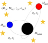 |
Fig. 1. Sketch of the IMBH–BH–BH triple configuration. We mark the main quantities that characterise the triple: IMBH mass (MIMBH), stellar BH masses (MBH1, 2), and orbital semimajor axis and eccentricity of the IMBH–BH1 (a1, e1) and IMBH–BH2 (a2, e2) systems, and those that characterise the host cluster: gravitational potential (ΦGC), total mass (MGC), typical radius (rGC), and velocity dispersion (σGC). |
We adopt four values of the IMBH mass, namely Log(MIMBH/M⊙) = 2, 3, 4, 5. This range covers typical values of putative IMBH masses forming in stellar systems of various sizes, from young and open clusters, to GCs, and up to nuclear clusters. We note that the lowest value taken for MIMBH will likely involve mergers with mass ratios of > 0.1; these therefore fall outside the range of IMRIs. Nonetheless, exploring the low end of the IMBH mass function will help us to better understand the perspectives of IMBH–BH mergers from the point of view of both low- (e.g., Will 2004; Amaro-Seoane 2018a) and high-frequency (e.g., Mandel et al. 2008; Gair et al. 2011; Abbott et al. 2017) GW detectors, especially in light of the recent discovery of GW190521, a GW source associated with the formation of an IMBH with a mass of 142 M⊙ (The LIGO Scientific Collaboration & the Virgo Collaboration 2020).
The properties of the cluster in which the IMBH is embedded, which define the cluster potential, are varied depending on the model. The cluster density profile is assumed to be either a Dehnen sphere with an inner slope of γGC = 0.5 (model S0, S3, S4, S5, S6) or 1.0 (model S1), or a Plummer sphere (model S2). In both cases, the cluster half-light radius is assumed to be Reff = 3.4 pc, namely the mean value of Milky Way GCs (Harris et al. 2014). The mass of the cluster is calculated via the scaling provided by Arca-Sedda (2016), connecting the host cluster mass MGC with the total ‘dark’ mass inhabiting the cluster centre, which is comprised of either an IMBH or a sizable population of stellar BHs:
 (1)
(1)
with α = 0.999 ± 0.001 and β = 2.23 ± 0.009. The typical cluster radius is therefore calculated from the assumed Reff and the adopted mass profile. Upon these assumptions, an IMBH with mass MIMBH = 102(105) M⊙ is associated with a cluster mass of MGC = 1.7 × 10⁴(1.7 × 10⁷) M⊙, and therefore our models ideally span the mass range of young clusters, GCs, nuclear clusters, and dwarf galaxy nuclei. We assume that the IMBH is orbited by two stellar BHs because the IMBH is expected to be the most massive object in the cluster and the dominant element in determining the dynamics. The choice of limiting the number of BH companions to two is dictated by the numerical evidence that IMBHs tend to form after the reservoir of the BH population is diminished severely through dynamical interactions (Portegies Zwart & McMillan 2002; Giersz et al. 2015). Compared to other works focusing on similar topics, our models do not rely on any preferential configuration or initial hierarchy for the IMBH–BH–BH system, because we expect the evolution around the IMBH to be mostly driven by the chaotic interactions involving the compact objects surrounding the IMBH (e.g., Konstantinidis et al. 2013).
We assume that the two BHs move on Keplerian orbits around the IMBH and that the centre of mass of the three BHs coincides with the cluster centre. We note that this choice allows the lower mass IMBHs to not necessarily be in the cluster centre at the beginning of the simulation. For each IMBH–BH orbit, we draw the orbital eccentricity e1, 2 from a thermal distribution P(e)de = 2ede (Plummer 1911). The semimajor axes of the two orbits are selected either from a distribution that is flat in logarithmic values limited to the range of a1, 2 = 0.1−104 AU (set S5) or according to the overall cluster mass distribution (S0-4 and S6) which for a Dehnen model is given by:
 (2)
(2)
where rGC = 4/3Reff(21/(3 − γ)−1) is the cluster scale radius (Dehnen 1993). In the latter case, the maximum semimajor axis allowed is given by the distance to the cluster centre at which the cluster mass is M(r) = 60 M⊙, which is twice the typical stellar BH mass (Spera & Mapelli 2017); therefore, inverting the equation above we get amax ≡ r(60 M⊙). This choice implies that increasing the cluster mass at fixed Reff leads to a smaller value of amax. For example, for MIMBH = 100(105) M⊙ we obtain amax = 20 000(200) AU. We note that the assumption on the semimajor axis distribution in S0-4 and S6 ensures that the initial position of the BHs follows the underlying mass distribution of the host cluster. As opposed to this, the assumption of a logarithmically flat a1, 2 distribution for S5 permits us to explore the role of the semimajor axis in determining IMRI formation.
The BH mass spectrum is also allowed to vary: we use the BH mass spectrum derived by Spera & Mapelli (2017, SM17), assuming a progenitor metallicity of Z = 0.0002 for models S0, S1, S2, and S5 and Z = 0.02 for model S6; a power-law mass spectrum with slope 2.2 (O’Leary et al. 2016, O16) in the range 3−30 M⊙ (model S3); or a flat distribution in the range 3−30 M⊙ (hereafter FLAT, model S4). The three different BH mass spectra adopted describe two possible situations: one in which the BH population reflects the original population of stars and another in which dynamics leads to selection on the BH mass distribution that is either mild (power-law distribution) or sufficiently strong to erase any memory of the original mass function (flat distribution).
All simulations are performed using ARGdf (Arca-Sedda & Capuzzo-Dolcetta 2019), a modified version of the ARCHAIN code that implements post-Newtonian (PN) dynamics and ‘algorithmic regularisation’ to handle close encounters and strong collisions (Mikkola & Tanikawa 1999; Mikkola & Merritt 2008). For our purposes, we include in our treatment only 1-, 2-, and 2.5-order PN terms. Additionally, ARGdf allows the user to take into account the gravitational field generated by the host stellar system and a dynamical friction term in particle equations of motion. Simulations are halted if: one of the two BHs merge with the IMBH, the two BHs merge together, one of the BHs is ejected, the simulated time exceeds t = 1 Gyr, or the runtime exceeds 1 h.
The reasoning behind the choice of a maximum simulation time of 1 Gyr is twofold. On the one hand, this is the typical timescale (evaporation time) over which the IMBH–BH systems might be disrupted because of interactions with passing stars, as explained in the following section. On the other hand, this limit enables us to maintain a good balance between computational load and data storage – the data required ∼4 Tb of storage space and around 2 months of computational time – and the reliability of the models. We note that carrying out the simulations for a time > 109 yr implies performing the BH orbit integration over 1 million times. Such long integration could lead to a considerable increase in integration error, despite the fact that the ARGdf code enables an accuracy over conserved quantities to a level of < 10−12. A summary of all models considered is provided in Table 1.
Main properties of our models.
3. Results
3.1. Formation and merger of intermediate-mass ratio inspirals
In this section we discuss the main results of our simulations. Hereafter, we refer to both IMBH–BH mergers and IMRIs indiscriminately although the smallest value of the IMBH mass adopted (102 M⊙) leads to IMBH–BH mergers with a mass ratio larger than expected for IMRIs. The outcomes of our simulations can be classified in three main categories:
(a) the IMBH–BH–BH system remains bound over the simulated time (bound, fbnd);
(b) one of the stellar BHs is ejected away leaving behind an IMBH–BH binary (disrupted, fdis);
(c) one of the BH merges with the IMBH (mergers, fIMRI).
Figure 2 provides a simplistic sketch of the possible outcomes of our simulations. Table 2 shows the percentage of models falling in each of these categories for the different models explored. On average, we note that mergers constitute fIMRI ∼ 20 − 32% of the models, with little dependence on the initial conditions assumed. Models falling in category (a) or (b) do not automatically exclude an IMBH–BH merger. In case (a), i.e. a bound IMBH–BH–BH, the triplet can be arranged in a configuration in which the IMBH is more tightly with one of the BHs while the other orbits around their common centre of mass. In this case, the triple can either evolve chaotically or undergo secular effects, such as the so-called Kozai-Lidov mechanism (Kozai 1962; Lidov 1962), which can trigger the eccentricity of the innermost IMBH–BH binary to grow to values close to unity.
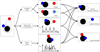 |
Fig. 2. Schematic view of IMBH–BH–BH triple evolution. |
Main results of N-body simulations.
In case (b), i.e. ejection of one of the stellar BHs, the evolution of the remaining IMBH–BH binary will be due to the sum of two contributions, namely energy removal from binary–single interactions and GW emission.
In both cases (a) and (b), binary–single interactions compromise the IMBH–BH survival over a typical evaporation time (Binney & Tremaine 2008; Stephan et al. 2016; Hoang et al. 2018):
 (3)
(3)
where m* is the average stellar mass in the nucleus, ρg is the stellar density, σg is the cluster velocity dispersion, and lnΛ = 6.5 is the Coulomb logarithm. In our simulations, the initial evaporation time ranges tev = 107 − 109 yr, depending on the orbital properties, the IMBH mass, and the cluster structure. If the IMBH–BH enters the IMRI phase, binary–single interactions are expected to play little to no effect in its evolution (Amaro-Seoane 2018a). In this case, the IMRI will continuously shrink, emitting GWs until coalescence, which takes place on a timescale of (Peters 1964)
 (4)
(4)
The long-term effect of multiple perturbers on the evolution of the IMBH–BH–BH system cannot be captured by our simulations; we therefore decided to exclude from the analysis all models in which the three bodies remain bound by the end of the simulation. We thus consider only systems falling in cases (b) and (c). In simulations where one BH is ejected (case b), we label the remaining IMBH–BH binary as a merger if tGW < tev, as these systems are likely to merge before dynamical encounters break them apart.
Table 2 summarises the main results of our simulations, highlighting the fraction of bound systems, disrupted systems, and mergers. As indicated in the table, we find a handful of models in which the two stellar BHs undergo a merger, whose number is Nbbh < 1 − 22. This effect is maximised in set S5 and for models with an IMBH mass of MIMBH = 100 − 1000 M⊙.
Clearly, while the categorisation provided suggests three well-separated classes, it must be noted that models falling in case (c), that is, mergers, might have undergone a chaotic triple phase, or secular effects that triggered the IMBH–BH merger. Figure 3 shows one such example: An IMBH with a mass of MIMBH = 102 M⊙ forms a tight binary with a stellar BH of MBH = 15 M⊙. The binary is subjected to perturbation of the outer BH with mass MBH = 5 M⊙ which causes a continuous oscillation of the eccentricity up to the point (case b) – around 300 Myr from the beginning of the simulation – at which the eccentricity peaks at values of ∼0.999998. Subsequently, GW emission kicks in and starts dominating the IMBH–BH binary evolution, eventually culminating in a merger (case c). The bottom panel in Fig. 3 shows the evolution of the same system in the absence of the external potential. It can be seen that when the external potential is not accounted for in the simulation, the three BHs undergo a faster evolution, which leads to the ejection of one BH on a timescale of < 2 Myr, leaving behind an IMBH–BH binary with a merger timescale of ∼1022 yr. In this case, the external potential facilitates the IMBH–BH merger by favouring a longer and more efficient interaction among the three BHs. Nonetheless, it must be noted that predicting the effect of an external potential on the evolution of the three bodies is not trivial, as it does not necessarily facilitate the binary merger (see e.g., Arca Sedda 2020; Petrovich & Antonini 2017).
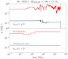 |
Fig. 3. Time-evolution of the semimajor axis (straight blue line) and eccentricity (dotted red line) for one of the simulations performed in S0. Panels show the case with (top panel) and without (bottom panel) the external potential of the cluster. |
As summarised in Table 2, the fraction of systems resulting in an IMRI depends on the IMBH mass and the model adopted. Figure 4 shows the fraction of mergers fIMRI as a function of the IMBH mass for different models. We see that the scatter among different models and for a fixed IMBH mass value is considerable, spanning from fIMRI ∼ 10% (S2) to 50% (S6) for MIMBH = 103 M⊙.
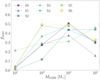 |
Fig. 4. Merger probability of IMRIs as a function of IMBH mass for all models explored. |
Despite the absence of a clear trend, our results suggest that the IMRI merger probability peaks at IMBH masses of MIMBH ∼ 104 M⊙, while it is limited to a few percent in the case where MIMBH = 100 M⊙. This is primarily due to the fact that models with MIMBH = 100 M⊙ have on average wider orbits, and can move more in the cluster potential compared to heavier IMBHs. Conversely, models with heavier IMBHs are characterised by initially tighter orbits, a deeper potential well, and the IMBH is less subjected to the Brownian motion thanks to its large inertia. This hypothesis is supported by the fact that in model S5, where the initial semimajor axis distribution is insensitive to the cluster mass, the merger fraction varies only slightly within the IMBH mass range MIMBH < 104 M⊙. We note that the majority of IMRIs formed in these models are triggered by the chaotic interactions between the three BHs, rather than by secular effects.
In the following section, we exploit these results to infer the cosmological merger rate of IMRIs associated with different IMBH mass ranges and GW detectors.
As shown in Fig. 5 for models S0-5 (different cluster density profile and BH mass spectrum) and Fig. 6 for models S0 and S6 (different stellar metallicity), another important property that can be inferred from our models is the mass distribution dN/dMBH of the IMRI secondary. Comparing S0, S1, and S3 – which differ only in the cluster density profile but adopt the same BH mass spectrum (Spera & Mapelli 2017) – it is apparent that the dN/dMBH does not depend on the environment, but rather on the BH mass spectrum adopted. In fact, the mass distribution in S0, S1, and S3 datasets shows a clearly bimodal distribution peaked at ∼7 M⊙ and 34 M⊙ which is directly inherited by the assumption that BH progenitor masses are distributed according to a Kroupa (2001) initial mass function and that the natal BH mass spectrum follows Spera & Mapelli (2017). The picture changes significantly if another BH mass spectrum is adopted. In the case of a power-law mass spectrum in the range MBH = 3−30 M⊙ we find that dN/dMBH declines sharply starting from 3 M⊙ and truncates at > 25 M⊙, whereas in the case of an initially flat mass spectrum the BH mass distribution increases toward 25 M⊙ and abruptly drops beyond this value.
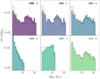 |
Fig. 5. Mass distribution of the IMRI secondary for models S0-5. Each colour corresponds to a different dataset to facilitate the comparison between different panels and figures. Dashed lines mark the mass function adopted for stellar BHs. |
Assuming smaller values for the initial semimajor axis (S5) does not significantly affect the merging BH mass distribution, which in that case resembles that obtained for S0-3. As shown in Fig. 6, increasing the stellar metallicity to solar values (S6) implies a reduction in the maximum value of the IMRI secondary mass to 25 M⊙.
Our models show that the mass distribution of the stellar-BH in the IMRI reflects the underlying BH mass spectrum, unless this is considerably flat. This suggests that the detection of IMRIs can help to unravel the features of BH populations residing in dense clusters. For instance, the double peak distribution apparent in S0-2 and S5 is essentially due to the stellar evolution recipes adopted for single stars. If dynamics is not responsible for significantly shaping the population of BHs around an IMBH, IMRIs can help us to unravel the stellar BH natal mass spectrum. On the other hand, if dynamics had enough time to significantly affect the BH population – for example causing the ejection of the most massive BHs via strong scattering – the detection of IMRIs can tell us more about these ‘BH burning’ mechanisms (see e.g., Kremer et al. 2020).
The distribution of merger times tmer –which are defined as the sum of the simulated time and the GW timescale evaluated through Eq. (4)– shown in Fig. 7 highlights a clear difference between the models in which the BH orbital parameters are selected according to the underlying cluster mass distribution (S0-4 and S6) and the model where the semimajor axes are drawn from a logarithmically flat distribution (S5). Whilst in the former case, tmer is broadly distributed in the range of 105 − 109 yr with a peak in correspondence of tmer ∼ 8 × 10⁸ yr, in the latter, the tmer distribution is generally flat in logarithmic values and extends down to 0.5 yr. This apparent difference owes to the adopted distribution of initial semimajor axis, which in S5 is logarithmically flat in the range 0.02−2 × 10⁴ AU, whilst in all the other models the boundary values depend on the cluster mass, which is directly linked to the IMBH mass. This is clearly shown in the bottom panel of Fig. 7, which compares the initial semimajor axis distribution adopted in the S5 and S0 datasets.
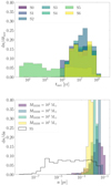 |
Fig. 7. Top panel: distribution of IMRI merging times calculated for all mergers in all the models explored. Different colours and symbols correspond to different model sets as indicated in the legend. Bottom panel: initial semimajor axis distribution in set S5 (black steps) and set S0 (filled steps). For the latter, we show the distribution for different values of the IMBH mass. |
3.2. Eccentricity of intermediate-mass ratio inspirals
An important parameter that could be inferred from IMRI observations is the eccentricity of the source, which may encode information about the IMRI formation channel. For instance, high eccentricities are thought to be the footprint of a dynamical origin, at least for stellar BH mergers (e.g., Nishizawa et al. 2016). To better understand whether our IMRI models are expected to retain significant eccentricity while sweeping across different GW observational bands, we show in Fig. 8 the average value of the eccentricity calculated when IMRIs cross the frequency windows (10−3 − 10−1 − 1−10) Hz for all simulation sets, which covers the full range of frequencies accessible to low- (LISA), intermediate- (DECIGO), and high-frequency (LIGO, ET) detectors. It is apparent that our IMRIs already have low eccentricity at mHz frequencies, where on average we find e = 10−4 − 0.03.
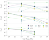 |
Fig. 8. Average eccentricity of IMRIs emitting in different frequency bands. From top to bottom, panels refer to f = 10−3 − 10−1 Hz, f = 10−1 − 1 Hz, f = 1−10 Hz, and f > 10 Hz. Different colours and symbols identify different models. |
Such low eccentricities are mainly due to the fact that the semimajor axis of the IMBH–BH merger is relatively large (i.e. ∼1−10 AU) at formation, which is when the effect of the third BH on the IMBH–BH evolution becomes negligible. This, in turn, is connected with the initial conditions adopted. We find that in S5, where we adopt a tighter range of semimajor axis compared to all other models, the eccentricity tends to be larger at all IMBH masses and at almost all frequencies.
Formation channels that are different from the one described here, such as gravitational captures or Kozai-Lidov resonances, tend to produce a non-negligible fraction of eccentric IMRIs. Therefore, measuring the eccentricity of an IMRI can help to constrain the mechanism leading to its formation. The possible formation of almost circular IMRIs that are within the range observable by GW instruments has implications for their detectability, as we show in Sect. 5.
3.3. Survival of intermediate-mass black holes in dense star clusters
Promptly after a merger event, the anisotropic emission of GWs can impart a recoil kick to the merger product, depending on the mass and spin of the two merging objects (Campanelli et al. 2007; González et al. 2007; Lousto & Zlochower 2008; Lousto et al. 2012), which can kick the IMBH out of the cluster (e.g., Holley-Bockelmann et al. 2008; Fragione et al. 2018), where it remains thereafter. This can significantly affect the retention probability of low-velocity dispersion (5 km s−1) star clusters, which is limited to 1−5% for BHs with masses of mBH ∼ 100 M⊙ that undergo one or two consecutive mergers (Arca Sedda et al. 2020b).
Assessing the retention probability for IMBHs is crucial in order to place constraints on their possible presence in star clusters. To explore this aspect, we performed a statistical analysis on our models to determine the retention probability of IMBHs that undergo an IMRI phase in star clusters. For each merger in any modelled set, we used the numerical relativity fitting formulae provided by Jiménez-Forteza et al. (2017) to calculate the remnant IMBH mass, spin, and effective spin parameter, and adopted Lousto et al. (2012) prescriptions to calculate the GW recoil kick following the implementation described in Arca Sedda et al. (2020b). As the kick is intrinsically linked to the direction and amplitude of the spin of the components, we proceed as follows. We assign an initial spin of either SIMBH = 0.01 or SIMBH = 0.99 to the IMBH so as to explore the regime of an almost non-rotating IMBH and that of a maximal IMBH, whereas for the stellar BH natal spin distribution we assume a Gaussian centred on SBH = 0.5 with a dispersion of 0.12.
The recoil velocity is compared with the escape velocity calculated in the centre of the host cluster, which can be derived from the adopted cluster potential, i.e.  , a quantity that can be connected to the cluster mass MGC, the half-mass radius Rh, and the inner slope of the density profile γ through a simple formula:
![Mathematical equation: $$ \begin{aligned} { v}_{\rm esc}^2 = {\left\{ \begin{array}{ll} \displaystyle {\frac{G M_{\rm GC}}{R_h (2-\gamma )[2^{1/(3-\gamma )} - 1]}},&\mathrm{ Dehnen\ (1993),} \\ \displaystyle {\frac{1.3 G M_{\rm GC}}{R_h}},&\mathrm{ Plummer\ (1915).} \end{array}\right.} \end{aligned} $$](/articles/aa/full_html/2021/08/aa37785-20/aa37785-20-eq6.gif) (5)
(5)
We find that the IMBH retention is ensured whenever its mass exceeds MIMBH ≥ 104 M⊙, because the host cluster escape velocity is expected to be in the range of 80−200 km s−1 and the recoil kick is generally limited to < 1 km s−1 because of the IMRI small mass ratio. However, the picture is more complicated for more modest IMBH masses.
Figure 9 shows the cumulative distribution of recoil kicks for all mergers with MIMBH = (102 − 103) M⊙ and assuming an IMBH initial spin SIMBH = 0.99. We note that the retention probability can be directly evaluated from the cumulative distribution through the fraction of objects with vkick < vesc.
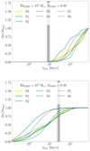 |
Fig. 9. Cumulative distribution of GW recoil kicks assuming an IMBH spin SIMBH = 0.99 and assuming an IMBH mass of MIMBH = 102 M⊙ (top) or MIMBH = 103 M⊙ (bottom). Different colours correspond to different model sets, and the shaded grey area encompasses the cluster central escape velocity. |
For low-mass IMBHs, MIMBH ∼ 100 M⊙, the retention probability remains below Pret = 0.5% if SIMBH = 0.99, and increases only slightly (Pret ≲ 1%) if the IMBH is slowly rotating (SIMBH = 0.01). We note that the retention probability weakly depends on the adopted cluster structure and stellar BH mass spectrum, suggesting that the retention of IMBH remnants with masses MIMBH ∼ 102 M⊙ in clusters masses of MGC ∼ 104 M⊙ is highly unlikely unless the host cluster central velocity dispersion exceeds 30 − 50 km s−1.
We note that assuming that the IMBHs with MIMBH = 102 M⊙ form in clusters ten times heavier than the adopted value (i.e. M ∼ 105 M⊙) has little impact on the retention probability. Indeed, adopting the range of escape velocities calculated for M = 1.7 × 10⁵ M⊙ clusters and assuming MIMBH = 100 M⊙ leads to a retention probability of Pret ∼ 10% in all model sets except S3, for which Pret ≲ 25%.
At IMBH masses of MIMBH ∼ 103 M⊙, instead, we see that the retention probability ranges between Pret = 75−99% depending on the adopted BH mass spectrum, with Pret reaching a maximum in the cases of S3, i.e. a power-law mass function, and S6, i.e. for BHs with solar-metallicity progenitors. In both cases, BH masses are lower than in other models on average, and therefore they will lead to IMRIs with smaller mass ratios that consequently receive smaller kicks. Our models suggest that in a population of metal-poor clusters with masses typical of GCs (i.e. > 105 M⊙), these have a more than 75% probability of retaining an IMRI remnant.
To further highlight the role of the stellar BH in determining the retention of the IMRI remnant, we proceeded as follows: (1) We divided the IMBH mass range – MIMBH = 102 − 5 × 10⁵ M⊙ – into 15 evenly distributed values in logarithmic scale. (2) For each IMBH mass, we created a sample of 100 stellar BHs whose masses are calculated following Spera & Mapelli (2017), assuming for the BH progenitors a Kroupa (2001) initial mass function and a metallicity of Z = 0.0002, i.e. the same adopted in models S0-2. (3) We assumed an IMBH spin of SIMBH = 0.99, whilst for the BH we extracted the spin from a Gaussian centred on SBH = 0.5 with a dispersion of 0.1. (4) Finally, we used the numerical relativity fitting formulae provided by Jiménez-Forteza et al. (2017) to calculate the IMRI merger remnant mass Mrem, spin Srem, and recoil velocity vkick, following the procedure depicted in Arca Sedda et al. (2020b). For each MIMBH − mBH pair, we repeated steps (3) and (4) 100 times, and for each of them we checked the vkick < vesc conditions, with vesc ranging between 10 and 250 km s−1 for the IMBH mass range MIMBH = 102 − 105 M⊙. The retention probability obtained through the procedure above is shown in Fig. 10.
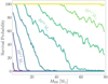 |
Fig. 10. IMBH retention probability as a function of the merging BH mass for different values of the IMBH mass identified by the colour coding. |
We find that an IMBH with mass MIMBH < 200 M⊙ gets ejected whenever the merging companion has a mass mBH ≥ 10 M⊙. Even for heavier IMBHs, for example MIMBH = 1000 M⊙, and thus heavier clusters, the retention probability rapidly drops below 50% if the companion mass exceeds MBH > 40 M⊙. The retention probability attains values > 80% regardless of the secondary BH mass only for much heavier IMBHs (MIMBH ∼ 104 M⊙).
The analysis above can be used to place constraints on the processes that might regulate IMBH seeding and growth. For instance, a scenario in which an IMBH forms through the merger of stellar-mass BHs seems highly unlikely in ‘normal’ star clusters, given the low retention fraction of IMBHs with masses MIMBH < 103 M⊙. However, if a substantial fraction of the IMBH is assembled via stellar accretion (e.g., Portegies Zwart & McMillan 2002; Giersz et al. 2015; Mapelli 2016; Di Carlo et al. 2019; Rizzuto et al. 2021), IMRI formation and merger would not represent a threat to the IMBH retention and further growth. In this sense, localising IMRIs with LISA and similar detectors could provide us with insights into the IMBH formation history and, more generally, IMBH formation mechanisms.
4. Evolution of intermediate-mass black holes in dense nuclear clusters
In this section, we investigate whether the effects of a merging event can be encoded in the remnant IMBH spin, and whether it is possible to use this quantity to infer IMBH evolutionary pathways. For each merger in all our models, we assign to the BH a spin drawn from a Gaussian distribution centred at SBH = 0.5 with a dispersion of 0.1, and we assume either an almost non-rotating (SIMBH = 0.01) or nearly extremal (SIMBH = 0.99) IMBH.
4.1. Spin evolution of intermediate-mass black holes
We find that a single merger event does not significantly affect the IMBH spin for mass values MIMBH > 104 M⊙, but it leaves a clear imprint on the spin of lighter IMBHs. Figure 11 shows the remnant spin for mergers in simulations assuming an IMBH mass of MIMBH = (102 − 103) M⊙ and spin SIMBH = (0.01 − 0.99). The panels make it clear that even a single merger event can significantly change the remnant IMBH spin.
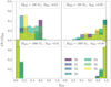 |
Fig. 11. Spin distribution of IMBH remnants in our simulations for all models and for IMBH masses of 102 M⊙ (top row) and 103 M⊙ (bottom row), assuming that the initial IMBH mass is either 0.01 (left column) or 0.99 (right column). |
In the case of low-mass, slowly spinning IMBHs (MIMBH, SIMBH = 102 M⊙, 0.01) the remnant IMBH spin can attain values as large as Srem = 0.8, while for rotating IMBHs the remnant spin shows a steep rise from 0.2 to 1. The difference is even more apparent in the case of MIMBH = 103 M⊙, because in this case the spin can increase to up to Srem = 0.2 if the IMBH is non-rotating, or reduce down to Srem = 0.8 if its initial spin is close to unity. This clear difference could unravel the history of the IMBH, in particular if the GW kick is sufficiently large to eject the remnant from the cluster and thus prevent it from undergoing further merger events.
However, it is worth exploring the possible changes to the spin of an IMBH initially formed in a cluster that is sufficiently large to retain the remnant after every merger. Figure 12 shows the spin variation of IMBHs with initial masses of MIMBH = 100, 300, 1000, or 5000 M⊙ and an initial spin of either SIMBH = 0.01 or 0.99, which undergo multiple mergers. The companion BH progenitor mass is extracted from a Kroupa IMF and the BH mass is taken from Spera & Mapelli (2017), whereas its spin is drawn by a Gaussian centred in SBH = 0.5 with a dispersion of 0.1. The plot makes clear that, regardless of the IMBH initial mass and spin, after a certain number of merging events the remnant spin tends to attain a value of Srem = 0 − 0.2. Such a result could have implications on the IMBH formation history. Let us assume a simple toy model in which an IMBH seed forms from stellar evolution, thus initially MIMBH ∼ 100 M⊙, and grows via multiple mergers with stellar BHs (the so-called hierarchical merger scenario). Assuming that the IMBH terminal mass is Mrem = 103 M⊙, which requires approximately 45 subsequent merger events, we would expect from Fig. 12 a final spin of Srem = 0.1 − 0.3. However, if the formation of a 103 M⊙ IMBH is driven by the direct collapse of a very massive star (Portegies Zwart & McMillan 2002; Giersz et al. 2015; Mapelli 2016) or the accretion of the very massive star onto a stellar BH (e.g., Rizzuto et al. 2021), the IMBH spin will be inevitably given by the process that determined either the collapse of the very massive star (VMS) or its accretion onto a stellar BH companion.
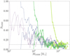 |
Fig. 12. Spin evolution for IMBH seeds that undergo a series of mergers with stellar BHs. The increase in mass marks the direction of time. The leftmost point in each curve represents the adopted values of the initial mass and spin of the IMBH. |
4.2. Seeding and growth of intermediate-mass black holes
In the previous sections we discuss how two stellar BHs can mediate the formation of an IMRI defined by an IMBH–BH binary, and how such a mechanism can affect the retention and the spin evolution of the remnant IMBH. In this section, we use the results from the previous sections to check whether or not the same mechanism could support the growth of an IMBH in a dense globular or nuclear cluster following the procedure schematised in Fig. 13 and described below.
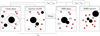 |
Fig. 13. Schematics of IMBH growth via three-body-driven IMBH–BH mergers. We assume that the three-body phase lasts for a duration of tmer, after which the third BH is ejected and the IMBH–BH binary either remains stable or undergoes an IMRI phase and ultimately merges, possibly kicking out the IMBH remnant owing to GW recoil. |
To this aim, we focus on an IMBH seed with a mass Mseed harboured in the centre of a star cluster with a central escape velocity vesc evaluated through Eq. (5). For our purposes, we adopt vesc = 100 km s−1. We note that this implies MGC > 3 × 10⁶ M⊙ and Rh < 3 pc, regardless of the value of the slope of the density profile or the type of model adopted (e.g., Dehnen 1993; Plummer 1911). We assume that the cluster forms t0 = 1 Gyr after the Big Bang, that is, at a redshift of z ∼ 5.53, and that an IMBH seed with mass Mseed and spin Sseed assemblies over a timescale of ∼100 Myr (Rizzuto et al. 2021).
In the following, we focus on S0 and S5, which share the same BH mass spectrum (Spera & Mapelli 2017) and metallicity (Z = 0.0002) but rely on different assumptions on the IMBH–BH initial orbits. We assume a seed mass of Mseed = (100 − 300 − 500) M⊙, and a spin of Sseed = 0.01 − 0.7 − 0.99. We create 500 merger trees for each combination, allowing up to a maximum of 103 interactions.
We assign the IMBH seed a companion BH with mass derived from the adopted mass spectrum and we assume that this binary undergoes perturbation from a third BH at a time tmer extracted from the distribution derived from the adopted set (either S0 or S5). We assume that such interaction results in IMRI formation and merger on a statistical basis, assuming a merging probability of pmer = 15%(30%), which is in agreement with the pmer value derived from our simulations for S0(S5). Specifically, we draw a number between pn = 0 and 1 and merge the IMBH and BH if pn < pmer; otherwise we assume that the IMBH–BH binary remains bound and another BH comes in and potentially triggers the IMBH–BH merger. We also assume that, if the merger fails, the IMBH has a 30% chance of exchanging the previous BH with a new one, as is suggested by our simulations. We note that the main difference between S0 and S5 is that in the latter the merger probability is larger and the merger time is widely distributed in the range 101 − 9 yr owing to the adopted distribution of semimajor axis.
In the case of a merger, we evaluate the recoil kick and remnant mass and spin after the merger. This procedure is repeated until either vkick > vesc, the time exceeds 13.8 Gyr, or the number of IMBH–BH interactions exceeds 103. The latter criterion is motivated by the fact that in a typical stellar population, the fraction of stars that collapse to a BH is ∼0.07 times the total number of stars, implying NBH ∼ 103 for a cluster with a mass of MGC = 106 M⊙ and an average stellar mass of m* = 0.7 M⊙. Although simple, this procedure enables us to rapidly check whether the mechanism studied in Sect. 3.1 is efficient enough to sustain the IMBH growth from stellar to intermediate scales.
Figure 14 shows a ‘merger tree’ for three cases in set S0, assuming an IMBH seed spin of Sseed = 0.7 and all the mass values considered. Comparison of the different models highlights the importance of IMBH seed mass in determining IMBH growth in this particular scenario. The growth of IMBH seeds with masses of Mseed = 100 M⊙ is generally limited to 20 − 50%, owing to the large GW recoil kicks that tend to eject the IMBH after a few merging episodes. This also limits the timescale over which IMBHs grow, which in our models tends to be shorter than 6 Gyr. In such a case, the three-body dynamics presented here would be inefficient in determining IMBH growth, which should thus proceed most likely via stellar accretion onto stellar-mass BHs (e.g., Giersz et al. 2015). However, if the initial mass of the IMBH seed is slightly larger, i.e. Mseed > 300 − 500 M⊙, the smaller GW recoil kick makes the IMBH growth via three-body dynamics easier, causing the IMBH in some cases to reach a final mass of MIMBH ≳ 103 M⊙ over 12 Gyr of evolution.
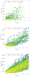 |
Fig. 14. Merger tree for IMBH seeds growing via three-body dynamics in a cluster with a central escape velocity of 100 km s−1. We show only 100 tracks for each panel for the sake of readability. Stellar BH masses are drawn from the mass distribution in Fig. 5 according to model set S0. Each track corresponds to a different model. We assume that the IMBH seeding and growth starts at redshift z = 2. |
However, GW recoil limits the likelihood for IMBHs to grow via IMBH–BH mergers. In order to quantify the IMBH growth ‘success’, we calculate the number of IMBHs that can be found at a given redshift normalised to the total number of IMBH seeds assumed. As shown in Fig. 15, only 2 − 3% of IMBH seeds with initial masses of Mseed = 100 M⊙ can grow and be observed at lower redshifts, whilst this percentage reaches ∼10% for heavier seeds (Mseed > 300 M⊙) and lower redshifts (z < 1), owing to the fact that larger seeds receive smaller kicks and thus have a greater probability of undergoing long merger chains.
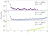 |
Fig. 15. Fraction of IMBHs at different redshift values normalised to the total number of IMBH seeds initialised at a redshift of z = 6. From top to bottom, panels refer to an initial seed with mass Mseed = (100, 300, 500) M⊙ and spin Sseed = 0.7. |
To explore how such a mechanism would impact a putative population of IMBHs over cosmic time, we repeated the procedure above extracting the IMBH seed mass in the range MIMBH = (100 − 500) M⊙ according to a power law with a slope of −2 and a spin according to a Gaussian peaking at SIMBH = 0.5, i.e. we assume that IMBH seeds and stellar BHs are characterised by the same spin distribution. For each model, we select the host cluster mass according to a power-law distribution with a slope of −2 in the range MGC = (105 − 5 × 10⁶) M⊙ (Zhang & Fall 1999; Gieles 2009; Larsen 2009; Chandar et al. 2010a,b, 2011), and we assign to all clusters a half mass radius of R = 2 pc and central slope of the density profile γ = 0.5. Also, we assume that the host cluster formed at a redshift that is extracted randomly in the range z = 2 − 6 (Katz & Ricotti 2013). Upon these assumptions, Fig. 16 shows the mass and spin distribution of IMBHs that underwent coalescence at least once as a function of redshift.
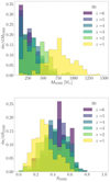 |
Fig. 16. Mass (top panel) and spin (bottom panel) distribution of IMBHs at different redshifts, assuming that the IMBH growth process is dominated by three-body interactions. Here we consider only IMBHs that underwent at least one merger. |
We see that at a redshift of z > 3, the IMBH mass and spin distributions roughly reflect the adopted ones, implying that mergers have little impact on IMBH seed mass, mostly because the number of repeated mergers at high redshifts is rather low, up to a few. At lower redshifts z ≤ 3, instead, multiple mergers affect the IMBH mass distribution significantly, leading the present-day IMBH mass distribution to acquire a very well-defined distribution peaked at MIMBH = 750 M⊙. Similarly, multiple mergers lead to a progressive decrease of the IMBH spin, whose distribution peaks around 0.3 at redshift z < 1. We note that we are considering here only IMBHs that merge with a stellar BH, and therefore the distribution in Fig. 16 represents the mass and spin distributions of IMBHs as seen via GW detection. The absence, in our model, of IMBHs with present-day masses larger than 1.5 × 10³ M⊙, is likely due to the adopted cluster mass distribution, which limits the number of heavy clusters capable of retaining the IMBH upon multiple mergers, and the neglection of the accretion of stars as a source of IMBH growth.
In this sense, our approach provides a simple picture of how an IMBH grows as it merges multiple times with stellar BHs. On the one hand, the absence of ‘smoking gun’ observations of IMBHs much heavier than 103 M⊙ in GCs would suggest that this IMBH–BH merger channel could be one of the main engines driving the (modest) IMBH growth. On the other hand, discovering the fingerprints of IMBHs with MIMBH ≫ 103 M⊙ would hint at a much more complex evolutionary scenario, where either the IMBH–BH merging process proceeds more efficiently compared to our model, or a substantial fraction of the IMBH mass is accreted through stellar feeding.
In the following sections, we exploit our model to predict the merger rate as it could be seen currently with LIGO, and in the near future with LISA, DECIGO, and the Einstein Telescope (ET).
5. Gravitational waves
5.1. Gravitational-wave signal
Our simulations encompass a wide range of IMRI models, encompassing the layer of ‘ordinary’ BH binaries (mass ratio q > 0.1) and approaching the limit of extreme-mass ratio inspirals (q < 3 × 10⁻⁵). This setup implies that the GW emission connected with our modelled mergers can populate a wide range of GW frequencies, from millihertz to decihertz. Figure 17 shows the characteristic amplitude of GWs (Kocsis et al. 2012; Arca-Sedda et al. 2021; Amaro-Seoane 2018a; Robson et al. 2019) as a function of their frequency for a sample of IMRIs with different IMBH mass, assuming an observation time of 4 yr and a source location of z = 0.1 (i.e. at a luminosity distance of DL ∼ 460 Mpc). We compare the modelled signal with the sensitivity curve of several detectors, namely LISA (Amaro-Seoane et al. 2013; Amaro-Seoane 2017), the advanced laser interferometer antenna (ALIA, Bender et al. 2013), the Deciherz Gravitational-Wave Observatory (DECIGO, Kawamura 2011), LIGO (Abbott et al. 2016), and the ET (Punturo et al. 2010). We see that mergers involving IMBHs with masses MIMBH < 105 M⊙ are promising multiband sources that can be seen in one detector during the inspiral phase and in another during the merger.
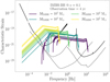 |
Fig. 17. Characteristic strain–frequency evolution for a sample of mergers in SET0. Each point in the plane refers to the signal associated with the IMRI dominant frequency. Different colours identify different IMBH masses (MIMBH). The calculated signal is overlaid on the sensitivity curve of several detectors, from lower to higher frequency: LISA and LIGO (straight black line), DECIGO and ET, and ALIA (dashed black line). |
5.2. Detecting IMBHs in Milky Way globular clusters and in the Large Magellanic Cloud
In this section, we exploit our results to investigate whether the current design of LISA provides enough sensitivity to unveil the presence of IMBHs in our closest neighbourhood. To perform such a study, we assume a nearly circular IMRI with an IMBH mass in the range 102 − 106 M⊙ and a BH companion weighing either 10 or 30 M⊙. We assume that the IMRI emission frequency is 1 mHz, corresponding to an orbital semimajor axis of 10−3 − 10−2 AU. The merger time for IMRIs in this configuration ranges between 100 and 104 yr, thus much larger than the observation time. Assuming 4 yr observation time, the IMRI frequency will not vary significantly, the frequency variation being Δlnf < 10−4. As noted by Robson et al. (2019), whenever the latter quantity remains below 0.5, a GW source should be treated as nearly stationary. Upon this assumption, the signal-to-noise ratio (S/N) can be written as
 (6)
(6)
where f is the source initial frequency, hn is the adimensional instrument sensitivity, and
with Tobs the observation time, ℳ the IMRI chirp mass, and DL the luminosity distance. We note that the relation above implies that the S/N scales with  . Figure 18 shows the S/N calculated for the LISA instrument for IMRIs with an initial frequency of f = 1 mHz and masses in the 102 − 106 M⊙ range, assuming a luminosity distance of DL = 8 kpc. We find that an IMRI with mass MIMRI = (30 + 103) M⊙ has an associated S/N of 20, whereas this quantity reaches 100 for a 104 M⊙ IMBH. These estimates suggest that LISA can play a crucial role in probing the existence of IMBHs in Milky Way star clusters.
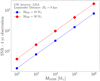 |
Fig. 18. Signal-to-noise ratio for several IMRIs assuming an initial frequency of 1 mHz, 4 yr of observation time, and a luminosity distance of DL = 8 kpc. |
Over the last decade a number of works have pointed out the potential presence of IMBHs in Galactic GCs, although in most cases the results were inconclusive. The family of clusters orbiting within less than 8 kpc from Earth includes several IMBH host candidates: 47Tuc (Kızıltan et al. 2017), NGC6266 (Abbate et al. 2019a), NGC6128 and NGC288 (Sollima et al. 2016), NGC6388, and NGC2808 (Miocchi 2007; Lanzoni et al. 2007).
However, whether these clusters actually host an IMBH is still an open question. For instance, the inferred value for the 47Tuc IMBH mass goes from MIMBH > 2000 M⊙ (Kızıltan et al. 2017) to substantially lower values of ≪1000 M⊙ (Abbate et al. 2019b), depending on the observational technique adopted. Similar arguments sustain the debates around other clusters, such as NGC6388 (Lanzoni et al. 2013; Lützgendorf et al. 2013). Therefore, LISA might play a crucial role in confirming the presence or absence of IMBHs in the Galaxy, at least in the closest GCs.
LISA may enable us to probe IMBHs in nearby galaxies. For instance, it was recently suggested that the Large Magellanic Cloud (LMC) might be harbouring an IMBH with a mass in the range 4 × 10³ − 104 M⊙ (Erkal et al. 2019) and up to 107 M⊙ (Boyce et al. 2017), while some of the clusters residing in the LMC could host IMBHs with masses in the range 103 − 104 M⊙ (Gualandris & Portegies Zwart 2007). Assuming a distance to the LMC of DL = 49.97 ± 1.13 kpc (Pietrzyński et al. 2013), we infer that LISA could detect Magellanic IMRIs with an S/N = 8 − 40, with the lower(upper) value corresponding to an IMBH with a mass of 103 M⊙(104 M⊙) and a BH companion of 30 M⊙.
5.3. Intermediate-mass ratio inspiral merger rate
The launch of LISA and the start of operations of the next generation of GW observatories like ET will enable us to unveil IMRIs at cosmological distances, provided that their number is sufficiently large to guarantee detection within the mission lifetime.
In the interest of predicting IMRI detectability, in this section we infer the merger rate for different detectors. To perform such calculations we need to account for the variation of galaxy number density across different redshifts z. The GW source ‘horizon’ determines the maximum distance in space, or the redshift zhor, at which the source signal is detected with a threshold S/N, namely:
 (7)
(7)
where f1, 2 is the initial and final frequency of the GW signal, hc(f, z) its characteristic strain, and Sn(f) its sensitivity. To determine zhor we integrate the final stage of the IMRI signal assuming an observation time of 4 yr, which is the nominal duration time of the LISA mission, and we assume an S/N of 15. We adopt the set of cosmological parameters measured by the Planck mission, namely H0 = 67.74 km s−1 Mpc−3, Ωm = 0.3089, ΩΛ = 0.6911 (Planck Collaboration XIII 2016). Moreover, we vary the IMBH mass in the range 50 − 106 M⊙ assuming that the companion has a mass of either 10 or 30 M⊙. Figure 19 shows how the horizon redshift changes for four different detectors: LIGO4, LISA5, DECIGO6, and ET7.
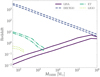 |
Fig. 19. Horizon redshift as a function of the IMBH mass assuming a BH companion with a mass of 10 M⊙ (lower curves) or 30 M⊙ (upper curves). Different curve collections correspond to different detectors: LISA (straight lines), DECIGO (dashed lines), ET (dotted lines), LIGO (dot-dashed lines). In the following section, we discuss whether some classes of IMRIs can appear as multiband sources. |
The plot shows that ground-based telescopes can provide insights into low-mass IMRIs (< 500 M⊙) up to redshift zhor ≤ 0.2. GW190521, a GW source recently detected by the LIGO-Virgo collaboration (The LIGO Scientific Collaboration & the Virgo Collaboration 2020; Abbott et al. 2021), could be one such low-mass IMRI, composed of a stellar BH with a mass of  and an IMBH with a mass of
  (see Nitz & Capano 2021). The ET will enable the observation of IMRIs with masses of < 103 M⊙ up to zhor = 1 − 10, whereas LISA will detect IMRIs with MIMBH = (104 − 105) M⊙ at the same redshift. As such, the potential synergy between ET and LISA could enable GW astronomers to fully cover the whole range of IMBH masses. Decihertz observatories like DECIGO (Kawamura 2011) and a similarly designed mission (Arca Sedda et al. 2020a) will push the observational limits beyond LISA and ET, enabling full coverage of the IMBH mass spectrum up to the dawn of the Universe, and providing an ideal means to unveil the true nature of IMBHs.
However, in the scenario explored here we assume that IMBHs form in GCs, and therefore the maximum redshift at which IMBH could be visible depends intrinsically on the typical timescales of star cluster formation. In the following, we adopt a maximum value of zmax = 6, corresponding to the formation epoch of the first stars, whenever zhor > zmax.
Once the dependence between the horizon redshift and the IMBH mass is determined, we can estimate the total number of IMRIs inside the cosmological volume encompassed by the horizon, NIMRI(zhor) ≡ NIMRI, a quantity that can be used to infer the IMRI merger rate. The NIMRI parameter can be expressed as:
 (8)
(8)
where dVc/dz is the comoving cosmological volume element, (1 + z)−1 the term that accounts for the dilation time, and dnIMRI/dMIMBH the number of IMRIs per unit of IMBH mass.
The latter term depends intrinsically on the interplay among galaxies, star clusters, and IMBH distribution within the cosmological volume. In the following, we pursue three different approaches to evaluate dnIMRI/dMIMBH and NIMRI, each implementing different assumptions about the distribution of IMBH hosts. In particular, the first approach (hereafter GAL) relies on the observed mass distribution of galaxies up to redshift z = 8 (Conselice et al. 2016), the second approach (hereafter CFR) relies on the assumption that the star cluster formation rate (CFR) is nearly constant in the range z = 2 − 8 and drops to zero at lower redshifts (Katz & Ricotti 2013), while the third approach (CSFE) relies on the cosmic star formation rate derived by Madau & Fragos (2017) and the cluster formation efficiency estimated by Bastian (2008).
In GAL we define
 (9)
(9)
Here, ξBH represents the probability that the IMBH will form a binary with a stellar BH, dn/(dMgdz) represents the number of galaxies per unit of redshift and galaxy mass, dn/dMGC is the number of clusters per cluster mass in a given galaxy, dMGC/dMIMBH connects GCs and IMBHs, nrep is the number of times that the same IMBH can form an IMRI with a stellar companion, fGW is the fraction of IMRIs that undergo a merger event within a Hubble time (a quantity that is extracted from our simulations; see Fig. 4), and pIMBH represents the probability that a cluster will host an IMBH. In the following, we assume pIMBH = 0.2 (Giersz et al. 2015).
In a typical ensemble of stars with masses following a Kroupa (2001) initial mass function, the number of stellar BH progenitors is a fraction of ∼10−3 of the whole population. In the absence of mass segregation and a mass spectrum, we might expect that the probability that an IMBH will be paired with a BH is simply 10−3. However, in real systems, mass-segregated stellar BHs tend to prevent other stars from migrating into the innermost cluster regions and thus they inhibit the IMBH in capturing other stellar types. The direct implication of the dominant effect of stellar BHs for the dynamics of the central cluster regions is a high probability that the IMBH will engage in a long-term relationship with a stellar BH rather than with a star, thus suggesting ξBH → 1.
The term dMGC/dMIMBH can be calculated by inverting Eq. (1) and performing the derivative. For the number distribution of the GC mass in a given galaxy, dn/dMGC, we assume a power-law
 (10)
(10)
with the slope s = 2.28 and the normalisation constant
Assuming Galactic values for the galaxy stellar mass, Mg = 6 × 10¹⁰ M⊙, and a star cluster mass range of MGC1, 2 = (5 × 10³ − 8 × 10⁶) M⊙, we calculate the corresponding IMBH mass range MIMBH ≃ (30 − 4.6 × 10⁴) M⊙ according to Eq. (1), which can also be used to write  9. The dn/(dMgdz) is obtained by exploiting the results in Conselice et al. (2016), who studied the distribution of galaxies with stellar masses up to 1012 M⊙ up to redshift z = 8. In particular, we exploit the following parametric expression of galaxy number density
 (11)
(11)
with ϕ*, α*, M* depending on the redshift (see Table 1 in Conselice et al. 2016), and M2 = 12.
Substituting all the terms and manipulating them conveniently, the total number of IMRIs in the portion of Universe accessible to a given detector is given by
 (12)
(12)
In both CFR and CSFE approaches, instead, we exploit the cosmological GC star formation rate ρSFR(z), which can be used to calculate the total number of GCs at a given redshift
 (13)
(13)
We note that t(z) expresses the dependence between time and redshift, and that the quantity ρSFR(z)t(z)/ < MGC> represents the total number of GCs formed within redshift z.
Given the power-law mass function for GCs used in the previous method, the normalisation factor in this case becomes
 (14)
(14)
and the total number of IMRIs inside a given cosmological volume is thus given by
 (15)
(15)
In CFR, we assume that ρSFR = 0.005 M⊙ yr−1 Mpc−3 in the range z = 2 − 6 (see Katz & Ricotti 2013), whereas in CSFE we assume that GCs form following the cosmic star formation rate derived by Madau & Fragos (2017) with an efficiency of ηGC = 0.08 (Bastian 2008), that is,
 (16)
(16)
with
![Mathematical equation: $$ \begin{aligned} \psi (z) = \frac{0.01(1+z)^{2.6}}{1+[(1+z)/3.2]^{6.2}} \,{M}_\odot \,\mathrm{yr}^{-1}\ \mathrm{Mpc}^{-3}. \end{aligned} $$](/articles/aa/full_html/2021/08/aa37785-20/aa37785-20-eq24.gif) (17)
(17)
The corresponding merger rate can be calculated as
 (18)
(18)
where ⟨T⟩ represents the median value of the IMRIs delay time, i.e. the time elapsed from GC formation to the IMRI coalescence. By definition, for a typical IMRI T is given by the sum of the cluster formation time tGC, f, the IMBH formation time tIMBH, f, and the IMRI merger time tmer. To estimate ⟨T⟩, we sample 2000 values of the triplet (tGC, f, tIMBH, f, tmer) as follows.
The GC formation time tGC, f is extracted according to either the GC formation rate derived by Katz & Ricotti (2013) or the cosmic formation rate derived by Madau & Fragos (2017). For the IMBH formation time tIMBH, f, we assume that one-third of IMBHs form via the rapid formation scenario whereas the remaining two-thirds form via the slow scenario described in Giersz et al. (2015). We therefore extract one-third of tIMBH, f values according to a uniform distribution limited within 0.05 − 1 Gyr, and the remaining in the range 1 − 10 Gyr. The IMRI merger time, instead, is sampled directly from our simulations (model S0). According to the procedure above, the median value of the IMRIs delay time is Log⟨T⟩ = 9.14 ± 1.22. Figure 20 shows the IMRI merger rate as a function of redshift calculated for different approaches, different ⟨T⟩ values, and for different instruments (LIGO, LISA, ET, and DECIGO).
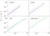 |
Fig. 20. Cumulative merger rate as a function of redshift for different detectors. Thick lines represent the results from GAL model, whereas the thin lines correspond to CFR and CSFE, assuming the mean value of the elapsed time. The dotted lines represent the upper(lower) bounds as determined by the minimum(maximum) value of ⟨T⟩. We assume that the BH companion in the IMRI has a mass MBH = 30 M⊙. |
The high uncertainties in ⟨T⟩ significantly affect our estimates. Assuming a Tobs = 4 yr long observation run, for LIGO we find a total merger rate of ΓIMRITobs ∼ 0.08 − 24 yr−1 out to a redshift of zhor, max = 0.57. At lower frequencies, LISA might record up to ΓIMRI ∼ 0.8 − 200 yr−1, pushing the limit for the IMBH mass to up to 40 000 M⊙ and thus allowing exploration of the mass range typical of IMRIs q ≃ 10−4. Comparing the theoretical properties of IMRIs forming in dense clusters with those forming in galactic nuclei (see e.g., Dayal et al. 2019) could help us in unravelling the intrinsic differences between these two classes of IMRIs and dissecting their presence in future LISA sources.
While the constraints on ‘present-day’ technologies are already encouraging, the next generation of both ground- and spaced-observatories could enable us to deliver a much larger number of observations up to the epoch of the formation of the first stars, thus allowing us to probe different IMBH formation mechanisms.
For instance, the ET could detect up to ΓIMRI ∼ 4 − 2000 yr−1 with masses MIMRI < 2000 M⊙, while space observatories sensitive at decihertz frequencies like DECIGO might record up to ΓIMRI ∼ 20 − 104 yr−1. Table 3 summarises the average IMRI rate values for the range of approaches and detectors adopted.
Main properties of our models.
6. Conclusions
In this work we explore one possible mechanism for the formation of IMRIs in dense GCs, namely the chaotic interaction among two BHs and one IMBH. Using a large set of N-body models, we studied how different properties (stellar BH mass spectrum, host cluster mass, IMBH mass) affect IMRI development. We exploited these models to investigate the possible implications for IMBH seeding and growth in dense clusters, and to infer the potential implications for present and future ground- and space-based GW detections. Our main results are summarised as follows.
-
The probability for IMRI formation and merger is significant, Pmer = 5 − 50%, and reaches maximum at larger values of the IMBH mass MIMBH.
-
The mass distribution of stellar BHs involved in merging IMRIs maps out the underlying stellar BH mass spectrum, suggesting that IMRIs are possible probes of the BH mass spectrum in dense clusters. A statistically significant number of IMRIs could tell us whether the BH mass spectrum in star clusters containing an IMBH preserves the original shape or is shaped by other mechanisms, such as for example the aforementioned BH burning via dynamical interactions.
-
Interestingly, this formation mechanism leads to IMRIs with generally low average eccentricities (e = 10−4 − 0.02) when sweeping through the GW frequency bands typical of low- (10−3 − 10−1 Hz), intermediate- (10−1 − 1 Hz) and high-frequency (1 − 100 Hz) detectors. The low eccentricity could be an indicator of this specific formation channel, as other scenarios (Kozai-Lidov resonant systems, hyperbolic encounters, gravitational captures) are expected to produce a consistent number of eccentric IMRIs.
-
We couple the results of the N-body models with a semi-analytic tool to explore the probability for IMRI remnants to be retained in their host clusters. We find that, because of GW recoil, only IMBHs with masses above MIMBH = 103 M⊙ have a significant retention probability (> 75%), provided that their companion BH mass is MBH < 45 M⊙. For lighter IMBHs (MIMBH ∼ 102 M⊙), we derive a retention fraction of smaller than 10%, regardless of the BH spin distribution and the IMBH spin.
-
For IMBHs with masses MIMBH < 103 M⊙, we show that even a single merger leaves an imprint on the spin of the remnant. In the case of Schwarzschild IMBHs, a merger with a stellar BH could increase the remnant spin to up to SIMBH = 0.7(0.2) for IMBHs with a mass of MIMBH = 102(103) M⊙. Similarly, for nearly extremal IMBHs, the spin after one single merger can decrease down to SIMBH = 0.8(0.2) in the same IMBH mass range.
-
The IMBH spin evolution is particularly interesting in the case of multiple mergers. We show that IMBHs growing via multiple mergers should exhibit low spins, generally SIMBH < 0.2. Thus, detecting IMRIs occurring in a star cluster would give us crucial insights into IMBH formation mechanisms: IMBHs formed via long merger chains show preferentially low spins, whilst those formed mostly via stellar feeding and collapse of massive stars are likely to follow the BH natal spin distribution.
-
We explore whether the IMRI formation channel discussed in this work could sustain the IMBH growth in dense globular or nuclear clusters. Using a semi-analytic tool to model IMBH evolution, we show that IMBH seeds heavier than Mseed > 300 M⊙ can grow up to MIMBH > 103 M⊙ via multiple mergers. Assuming that such seeds form at redshifts of z ∼ 2 − 6, we predict that around 1 − 5% of them will reach typical masses of ∼500 − 1500 M⊙ at a redshift of z = 0 in massive GCs, and will be characterised by relatively low spins, SIMBH ∼ 0.3.
-
We show that LISA can detect IMRIs in Milky Way GCs with a S/N of up to 10 − 100, and in Large Magellanic Cloud clusters with an S/N = 8 − 40.
-
We derive the IMRI merger rate for several detectors: LIGO (ΓLIGO = 0.003 − 1.6 yr−1), LISA (ΓLISA = 0.02 − 60 yr−1), ET (ΓET = 1 − 600 yr−1), and DECIGO (ΓDECIGO = 6 − 3000 yr−1).
The simulations presented here provide a comprehensive overview of the properties of IMBHs grown via repeated mergers in dense star clusters. Comparing these properties with future observations of IMRIs would help us to disentangle different IMBH formation scenarios. Our merger estimates highlight how the future synergy among GW detectors will enable us to fully cover the mass range bridging stellar BHs and SMBHs.
We find that the choice of stellar BH natal spin distribution does not significantly affect the results.
In agreement with the scenario in which GCs likely formed through redshift z = 2 − 6 (e.g., Forbes & Bridges 2010; VandenBerg et al. 2013)
We note that this is compatible with the expected initial mass function of young and old star clusters in galaxies (e.g., Gieles 2009).
The parameters a, b are obtained by manipulating Eq. (1).
Acknowledgments
MAS acknowledges the Alexander von Humboldt Foundation for the financial support provided in the framework of the research program “The evolution of black holes from stellar to galactic scales”, the Volkswagen Foundation Trilateral Partnership project No. I/97778 “Dynamical Mechanisms of Accretion in Galactic Nuclei”, and the Sonderforschungsbereich SFB 881 “The Milky Way System” – Project-ID 138713538 – funded by the German Research Foundation (DFG). PAS acknowledges support from the Ramón y Cajal Programme of the Ministry of Economy, Industry and Competitiveness of Spain. This work was supported by the National Key R&D Program of China (2016YFA0400702) and the National Science Foundation of China (11873022, 11991053). The authors acknowledge support from the COST Action GWverse CA16104. The authors acknowledge the use of the Kepler computer at ARI Heidelberg, funded by Volkswagen Foundation through the project GRACE 2: “Scientific simulations using programmable hardware” (VW grants I84678/84680), and the bwForCluster of the Baden-Württemberg’s High Performance Computing (HPC) facilities, which is supported by the state of Baden-Württemberg through bwHPC and the German Research Foundation (DFG) through grant INST 35/1134-1 FUGG.
References
- Abbate, F., Possenti, A., Colpi, M., & Spera, M. 2019a, ApJ, 884, L9 [Google Scholar]
- Abbate, F., Spera, M., & Colpi, M. 2019b, MNRAS, 487, 769 [Google Scholar]
- Abbott, B. P., Abbott, R., Abbott, T. D., et al. 2016, Phys. Rev. Lett., 116, 061102 [Google Scholar]
- Abbott, B. P., Abbott, R., Abbott, T. D., et al. 2017, Phys. Rev. D, 96, 022001 [Google Scholar]
- Abbott, R., Abbott, T. D., & Abraham, S. E. 2021, Phys. Rev. X, 11, 021053 [Google Scholar]
- Amaro-Seoane, P. 2018a, Liv. Rev. Rel., 21, 4 [Google Scholar]
- Amaro-Seoane, P. 2018b, Phys. Rev. D, 98, 063018 [Google Scholar]
- Amaro-Seoane, P., Gair, J. R., Freitag, M., et al. 2007, CQG, 24, R113 [Google Scholar]
- Amaro-Seoane, P., Aoudia, S., Babak, S., et al. 2013, GW Notes, 6, 4 [Google Scholar]
- Amaro-Seoane, P., Audley, H., Babak, S., et al. 2017, ArXiv e-prints [arXiv:1702.00786] [Google Scholar]
- Arca-Sedda, M. 2016, MNRAS, 455, 35 [NASA ADS] [CrossRef] [Google Scholar]
- Arca Sedda, M. 2020, ApJ, 891, 47 [Google Scholar]
- Arca Sedda, M., Askar, A., & Giersz, M. 2018, MNRAS, 479, 4652 [NASA ADS] [CrossRef] [Google Scholar]
- Arca-Sedda, M., & Capuzzo-Dolcetta, R. 2019, MNRAS, 483, 152 [NASA ADS] [CrossRef] [Google Scholar]
- Arca Sedda, M., Askar, A., & Giersz, M. 2019, MNRAS, submitted, [arXiv:1905.00902] [Google Scholar]
- Arca Sedda, M., Mapelli, M., Spera, M., Benacquista, M., & Giacobbo, N. 2020a, ApJ, 894, 133 [CrossRef] [Google Scholar]
- Arca Sedda, M., Berry, C. P. L., Jani, K., et al. 2020b, CQG, 37, 215011 [Google Scholar]
- Arca-Sedda, M., Li, G., & Kocsis, B. 2021, A&A, 650, A189 [EDP Sciences] [Google Scholar]
- Askar, A., Arca Sedda, M., & Giersz, M. 2018, MNRAS, 478, 1844 [NASA ADS] [CrossRef] [Google Scholar]
- Bastian, N. 2008, MNRAS, 390, 759 [NASA ADS] [CrossRef] [Google Scholar]
- Baumgardt, H. 2017, MNRAS, 464, 2174 [Google Scholar]
- Bellovary, J. M., Governato, F., Quinn, T. R., et al. 2010, ApJ, 721, L148 [NASA ADS] [CrossRef] [Google Scholar]
- Bellovary, J., Volonteri, M., Governato, F., et al. 2011, ApJ, 742, 13 [Google Scholar]
- Bender, P. L., Begelman, M. C., & Gair, J. R. 2013, CQG, 30, 165017 [Google Scholar]
- Binney, J., & Tremaine, S. 2008, Galactic Dynamics Second Edition (Princeton University Press) [Google Scholar]
- Boyce, H., Lützgendorf, N., van der Marel, R. P., et al. 2017, ApJ, 846, 14 [Google Scholar]
- Bromm, V., Coppi, P. S., & Larson, R. B. 2002, ApJ, 564, 23 [Google Scholar]
- Campanelli, M., Lousto, C. O., Zlochower, Y., & Merritt, D. 2007, Phys. Rev. Lett., 98, 231102 [Google Scholar]
- Chandar, R., Fall, S. M., & Whitmore, B. C. 2010a, ApJ, 711, 1263 [Google Scholar]
- Chandar, R., Whitmore, B. C., Kim, H., et al. 2010b, ApJ, 719, 966 [Google Scholar]
- Chandar, R., Whitmore, B. C., Calzetti, D., et al. 2011, ApJ, 727, 88 [Google Scholar]
- Conselice, C. J., Wilkinson, A., Duncan, K., & Mortlock, A. 2016, ApJ, 830, 83 [Google Scholar]
- Dayal, P., Rossi, E. M., Shiralilou, B., et al. 2019, MNRAS, 486, 2336 [Google Scholar]
- Dehnen, W. 1993, MNRAS, 265, 250 [NASA ADS] [CrossRef] [Google Scholar]
- Di Carlo, U. N., Giacobbo, N., Mapelli, M., et al. 2019, MNRAS, 487, 2947 [NASA ADS] [CrossRef] [Google Scholar]
- Erkal, D., Boubert, D., Gualandris, A., Evans, N. W., & Antonini, F. 2019, MNRAS, 483, 2007 [CrossRef] [Google Scholar]
- Forbes, D. A., & Bridges, T. 2010, MNRAS, 404, 1203 [NASA ADS] [Google Scholar]
- Fragione, G., Ginsburg, I., & Kocsis, B. 2018, ApJ, 856, 92 [NASA ADS] [CrossRef] [Google Scholar]
- Freitag, M., Amaro-Seoane, P., & Kalogera, V. 2006a, ApJ, 649, 91 [NASA ADS] [CrossRef] [Google Scholar]
- Freitag, M., Gürkan, M. A., & Rasio, F. A. 2006b, MNRAS, 368, 141 [NASA ADS] [Google Scholar]
- Gair, J. R., Mandel, I., Miller, M. C., & Volonteri, M. 2011, Gen. Rel. Grav., 43, 485 [CrossRef] [Google Scholar]
- Gieles, M. 2009, MNRAS, 394, 2113 [NASA ADS] [CrossRef] [Google Scholar]
- Giersz, M., Leigh, N., Hypki, A., Lützgendorf, N., & Askar, A. 2015, MNRAS, 454, 3150 [NASA ADS] [CrossRef] [Google Scholar]
- González, J. A., Sperhake, U., Brügmann, B., Hannam, M., & Husa, S. 2007, Phys. Rev. Lett., 98, 091101 [NASA ADS] [CrossRef] [MathSciNet] [PubMed] [Google Scholar]
- González, E., Kremer, K., Chatterjee, S., et al. 2021, ApJ, 908, L29 [CrossRef] [Google Scholar]
- Greene, J. E., Strader, J., & Ho, L. C. 2020, ARA&A, 58, 257 [CrossRef] [Google Scholar]
- Gualandris, A., & Portegies Zwart, S. 2007, MNRAS, 376, L29 [NASA ADS] [CrossRef] [Google Scholar]
- Harris, W. E., Morningstar, W., Gnedin, O. Y., et al. 2014, ApJ, 797, 128 [NASA ADS] [CrossRef] [Google Scholar]
- Haster, C.-J., Antonini, F., Kalogera, V., & Mandel, I. 2016, ApJ, 832, 192 [CrossRef] [Google Scholar]
- Hoang, B.-M., Naoz, S., Kocsis, B., Rasio, F. A., & Dosopoulou, F. 2018, ApJ, 856, 140 [NASA ADS] [CrossRef] [Google Scholar]
- Holley-Bockelmann, K., Gültekin, K., Shoemaker, D., & Yunes, N. 2008, ApJ, 686, 829 [NASA ADS] [CrossRef] [Google Scholar]
- Huang, S., Gong, X., Xu, P., et al. 2017, Sci. Sin. Phys. Mech. Astron., 47, 010404 [CrossRef] [Google Scholar]
- Jiménez-Forteza, X., Keitel, D., Husa, S., et al. 2017, Phys. Rev. D, 95, 064024 [CrossRef] [Google Scholar]
- Katz, H., & Ricotti, M. 2013, MNRAS, 432, 3250 [NASA ADS] [CrossRef] [Google Scholar]
- Kawamura, S., Ando, M., Seto, N., et al. 2011, CQG, 28, 094011 [CrossRef] [Google Scholar]
- Kızıltan, B., Baumgardt, H., & Loeb, A. 2017, Nature, 542, 203 [Google Scholar]
- Kocsis, B., Ray, A., & Portegies Zwart, S. 2012, ApJ, 752, 67 [CrossRef] [Google Scholar]
- Konstantinidis, S., Amaro-Seoane, P., & Kokkotas, K. D. 2013, A&A, 557, A135 [CrossRef] [EDP Sciences] [Google Scholar]
- Kozai, Y. 1962, ApJ, 67, 591 [NASA ADS] [CrossRef] [MathSciNet] [Google Scholar]
- Kremer, K., Ye, C. S., Chatterjee, S., Rodriguez, C. L., & Rasio, F. A. 2020, in Star Clusters: From the Milky Way to the Early Universe, eds. A. Bragaglia, M. Davies, A. Sills, & E. Vesperini, 351, 357 [Google Scholar]
- Kroupa, P. 2001, MNRAS, 322, 231 [NASA ADS] [CrossRef] [Google Scholar]
- Lanzoni, B., Dalessandro, E., Ferraro, F. R., et al. 2007, ApJ, 668, L139 [NASA ADS] [CrossRef] [Google Scholar]
- Lanzoni, B., Mucciarelli, A., Origlia, L., et al. 2013, ApJ, 769, 107 [NASA ADS] [CrossRef] [Google Scholar]
- Larsen, S. S. 2009, A&A, 494, 539 [NASA ADS] [CrossRef] [EDP Sciences] [Google Scholar]
- Latif, M. A., Schleicher, D. R. G., Schmidt, W., & Niemeyer, J. 2013, MNRAS, 433, 1607 [NASA ADS] [CrossRef] [Google Scholar]
- Leigh, N. W. C., Lützgendorf, N., Geller, A. M., et al. 2014, MNRAS, 444, 29 [CrossRef] [Google Scholar]
- Lidov, M. L. 1962, Planet. Space Sci., 9, 719 [Google Scholar]
- Lousto, C. O., & Zlochower, Y. 2008, Phys. Rev. D, 77, 044028 [CrossRef] [Google Scholar]
- Lousto, C. O., Zlochower, Y., Dotti, M., & Volonteri, M. 2012, Phys. Rev. D, 85, 084015 [NASA ADS] [CrossRef] [Google Scholar]
- Lu, J. R., Do, T., Ghez, A. M., et al. 2013, ApJ, 764, 155 [NASA ADS] [CrossRef] [Google Scholar]
- Luo, J., Chen, L.-S., Duan, H.-Z., et al. 2016, CQG, 33, 035010 [CrossRef] [Google Scholar]
- Lützgendorf, N., Kissler-Patig, M., Gebhardt, K., et al. 2013, A&A, 552, A49 [NASA ADS] [CrossRef] [EDP Sciences] [Google Scholar]
- MacLeod, M., Trenti, M., & Ramirez-Ruiz, E. 2016, ApJ, 819, 70 [CrossRef] [Google Scholar]
- Madau, P., & Fragos, T. 2017, ApJ, 840, 39 [NASA ADS] [CrossRef] [Google Scholar]
- Madau, P., & Rees, M. J. 2001, ApJ, 551, L27 [NASA ADS] [CrossRef] [Google Scholar]
- Mandel, I., Brown, D. A., Gair, J. R., & Miller, M. C. 2008, ApJ, 681, 1431 [CrossRef] [Google Scholar]
- Mapelli, M. 2016, MNRAS, 459, 3432 [NASA ADS] [CrossRef] [Google Scholar]
- McKernan, B., Ford, K. E. S., Lyra, W., & Perets, H. B. 2012, MNRAS, 425, 460 [CrossRef] [Google Scholar]
- Mezcua, M. 2017, Int. J. Mod. Phys. D, 26, 1730021 [Google Scholar]
- Mikkola, S., & Merritt, D. 2008, ApJ, 135, 2398 [NASA ADS] [CrossRef] [Google Scholar]
- Mikkola, S., & Tanikawa, K. 1999, MNRAS, 310, 745 [CrossRef] [Google Scholar]
- Miocchi, P. 2007, MNRAS, 381, 103 [NASA ADS] [CrossRef] [Google Scholar]
- Nishizawa, A., Berti, E., Klein, A., & Sesana, A. 2016, Phys. Rev. D, 94, 064020 [CrossRef] [Google Scholar]
- Nitz, A. H., & Capano, C. D. 2021, ApJ, 907, L9 [CrossRef] [Google Scholar]
- Noyola, E., Gebhardt, K., Kissler-Patig, M., et al. 2010, ApJ, 719, L60 [NASA ADS] [CrossRef] [Google Scholar]
- Ohkubo, T., Nomoto, K., Umeda, H., Yoshida, N., & Tsuruta, S. 2009, ApJ, 706, 1184 [NASA ADS] [CrossRef] [Google Scholar]
- O’Leary, R. M., Meiron, Y., & Kocsis, B. 2016, ApJ, 824, L12 [CrossRef] [Google Scholar]
- Peters, P. C. 1964, Phys. Rev., 136, B1224 [NASA ADS] [CrossRef] [Google Scholar]
- Petrovich, C., & Antonini, F. 2017, ApJ, 846, 146 [NASA ADS] [CrossRef] [Google Scholar]
- Pietrzyński, G., Graczyk, D., Gieren, W., et al. 2013, Nature, 495, 76 [NASA ADS] [CrossRef] [PubMed] [Google Scholar]
- Planck Collaboration XIII. 2016, A&A, 594, A13 [NASA ADS] [CrossRef] [EDP Sciences] [Google Scholar]
- Plummer, H. C. 1911, MNRAS, 71, 460 [CrossRef] [Google Scholar]
- Portegies Zwart, S. F., & McMillan, S. L. W. 2002, ApJ, 576, 899 [NASA ADS] [CrossRef] [Google Scholar]
- Punturo, M., Abernathy, M., Acernese, F., et al. 2010, CQG, 27, 084007 [CrossRef] [Google Scholar]
- Rizzuto, F. P., Naab, T., Spurzem, R., et al. 2021, MNRAS, 501, 5257 [CrossRef] [Google Scholar]
- Robson, T., Cornish, N. J., & Liu, C. 2019, CQG, 36, 105011 [NASA ADS] [CrossRef] [Google Scholar]
- Sollima, A., Ferraro, F. R., Lovisi, L., et al. 2016, MNRAS, 462, 1937 [CrossRef] [Google Scholar]
- Spera, M., & Mapelli, M. 2017, MNRAS, 470, 4739 [Google Scholar]
- Stephan, A. P., Naoz, S., Ghez, A. M., et al. 2016, MNRAS, 460, 3494 [NASA ADS] [CrossRef] [Google Scholar]
- Taniguchi, Y., Shioya, Y., Tsuru, T. G., & Ikeuchi, S. 2000, PASJ, 52, 533 [CrossRef] [Google Scholar]
- The LIGO Scientific Collaboration, & the Virgo Collaboration (Abbott, R., et al.) 2020, Phys. Rev. Lett., 125, 101102 [CrossRef] [Google Scholar]
- van der Marel, R. P., & Anderson, J. 2010, ApJ, 710, 1063 [Google Scholar]
- VandenBerg, D. A., Brogaard, K., Leaman, R., & Casagrande, L. 2013, ApJ, 775, 134 [NASA ADS] [CrossRef] [Google Scholar]
- Weatherford, N. C., Chatterjee, S., Rodriguez, C. L., & Rasio, F. A. 2018, ApJ, 864, 13 [NASA ADS] [CrossRef] [Google Scholar]
- Will, C. M. 2004, ApJ, 611, 1080 [CrossRef] [Google Scholar]
- Zhang, Q., & Fall, S. M. 1999, ApJ, 527, L81 [NASA ADS] [CrossRef] [PubMed] [Google Scholar]
- Zocchi, A., Gieles, M., & Hénault-Brunet, V. 2015, Star Clusters and Black Holes in Galaxies across Cosmic Time, Proceedings of the International Astronomical Union, IAU Symp., 312, 197 [Google Scholar]
All Tables
All Figures
|
Fig. 1. Sketch of the IMBH–BH–BH triple configuration. We mark the main quantities that characterise the triple: IMBH mass (MIMBH), stellar BH masses (MBH1, 2), and orbital semimajor axis and eccentricity of the IMBH–BH1 (a1, e1) and IMBH–BH2 (a2, e2) systems, and those that characterise the host cluster: gravitational potential (ΦGC), total mass (MGC), typical radius (rGC), and velocity dispersion (σGC). |
| In the text | |
|
Fig. 2. Schematic view of IMBH–BH–BH triple evolution. |
| In the text | |
|
Fig. 3. Time-evolution of the semimajor axis (straight blue line) and eccentricity (dotted red line) for one of the simulations performed in S0. Panels show the case with (top panel) and without (bottom panel) the external potential of the cluster. |
| In the text | |
|
Fig. 4. Merger probability of IMRIs as a function of IMBH mass for all models explored. |
| In the text | |
|
Fig. 5. Mass distribution of the IMRI secondary for models S0-5. Each colour corresponds to a different dataset to facilitate the comparison between different panels and figures. Dashed lines mark the mass function adopted for stellar BHs. |
| In the text | |
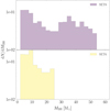 |
Fig. 6. As in Fig. 5, but for datasets S0 and S6. Here we show only the masses of merging BHs. |
| In the text | |
|
Fig. 7. Top panel: distribution of IMRI merging times calculated for all mergers in all the models explored. Different colours and symbols correspond to different model sets as indicated in the legend. Bottom panel: initial semimajor axis distribution in set S5 (black steps) and set S0 (filled steps). For the latter, we show the distribution for different values of the IMBH mass. |
| In the text | |
|
Fig. 8. Average eccentricity of IMRIs emitting in different frequency bands. From top to bottom, panels refer to f = 10−3 − 10−1 Hz, f = 10−1 − 1 Hz, f = 1−10 Hz, and f > 10 Hz. Different colours and symbols identify different models. |
| In the text | |
|
Fig. 9. Cumulative distribution of GW recoil kicks assuming an IMBH spin SIMBH = 0.99 and assuming an IMBH mass of MIMBH = 102 M⊙ (top) or MIMBH = 103 M⊙ (bottom). Different colours correspond to different model sets, and the shaded grey area encompasses the cluster central escape velocity. |
| In the text | |
|
Fig. 10. IMBH retention probability as a function of the merging BH mass for different values of the IMBH mass identified by the colour coding. |
| In the text | |
|
Fig. 11. Spin distribution of IMBH remnants in our simulations for all models and for IMBH masses of 102 M⊙ (top row) and 103 M⊙ (bottom row), assuming that the initial IMBH mass is either 0.01 (left column) or 0.99 (right column). |
| In the text | |
|
Fig. 12. Spin evolution for IMBH seeds that undergo a series of mergers with stellar BHs. The increase in mass marks the direction of time. The leftmost point in each curve represents the adopted values of the initial mass and spin of the IMBH. |
| In the text | |
|
Fig. 13. Schematics of IMBH growth via three-body-driven IMBH–BH mergers. We assume that the three-body phase lasts for a duration of tmer, after which the third BH is ejected and the IMBH–BH binary either remains stable or undergoes an IMRI phase and ultimately merges, possibly kicking out the IMBH remnant owing to GW recoil. |
| In the text | |
|
Fig. 14. Merger tree for IMBH seeds growing via three-body dynamics in a cluster with a central escape velocity of 100 km s−1. We show only 100 tracks for each panel for the sake of readability. Stellar BH masses are drawn from the mass distribution in Fig. 5 according to model set S0. Each track corresponds to a different model. We assume that the IMBH seeding and growth starts at redshift z = 2. |
| In the text | |
|
Fig. 15. Fraction of IMBHs at different redshift values normalised to the total number of IMBH seeds initialised at a redshift of z = 6. From top to bottom, panels refer to an initial seed with mass Mseed = (100, 300, 500) M⊙ and spin Sseed = 0.7. |
| In the text | |
|
Fig. 16. Mass (top panel) and spin (bottom panel) distribution of IMBHs at different redshifts, assuming that the IMBH growth process is dominated by three-body interactions. Here we consider only IMBHs that underwent at least one merger. |
| In the text | |
|
Fig. 17. Characteristic strain–frequency evolution for a sample of mergers in SET0. Each point in the plane refers to the signal associated with the IMRI dominant frequency. Different colours identify different IMBH masses (MIMBH). The calculated signal is overlaid on the sensitivity curve of several detectors, from lower to higher frequency: LISA and LIGO (straight black line), DECIGO and ET, and ALIA (dashed black line). |
| In the text | |
|
Fig. 18. Signal-to-noise ratio for several IMRIs assuming an initial frequency of 1 mHz, 4 yr of observation time, and a luminosity distance of DL = 8 kpc. |
| In the text | |
|
Fig. 19. Horizon redshift as a function of the IMBH mass assuming a BH companion with a mass of 10 M⊙ (lower curves) or 30 M⊙ (upper curves). Different curve collections correspond to different detectors: LISA (straight lines), DECIGO (dashed lines), ET (dotted lines), LIGO (dot-dashed lines). In the following section, we discuss whether some classes of IMRIs can appear as multiband sources. |
| In the text | |
|
Fig. 20. Cumulative merger rate as a function of redshift for different detectors. Thick lines represent the results from GAL model, whereas the thin lines correspond to CFR and CSFE, assuming the mean value of the elapsed time. The dotted lines represent the upper(lower) bounds as determined by the minimum(maximum) value of ⟨T⟩. We assume that the BH companion in the IMRI has a mass MBH = 30 M⊙. |
| In the text | |
Current usage metrics show cumulative count of Article Views (full-text article views including HTML views, PDF and ePub downloads, according to the available data) and Abstracts Views on Vision4Press platform.
Data correspond to usage on the plateform after 2015. The current usage metrics is available 48-96 hours after online publication and is updated daily on week days.
Initial download of the metrics may take a while.