| Issue |
A&A
Volume 651, July 2021
|
|
|---|---|---|
| Article Number | A118 | |
| Number of page(s) | 9 | |
| Section | The Sun and the Heliosphere | |
| DOI | https://doi.org/10.1051/0004-6361/202140427 | |
| Published online | 29 July 2021 | |
Harmonic electron-cyclotron maser emissions driven by energetic electrons of the horseshoe distribution with application to solar radio spikes⋆
1
Institute of Space Sciences, Shandong University, Shandong, PR China
e-mail: yaochen@sdu.edu.cn
2
Institute of Frontier and Interdisciplinary Science, Shandong University, Shandong, PR China
Received:
27
January
2021
Accepted:
11
May
2021
Context. Electron-cyclotron maser emission (ECME) is the favored mechanism for solar radio spikes and has been investigated extensively since the 1980s. Most studies relevant to solar spikes employ a loss-cone-type distribution of energetic electrons, generating waves mainly in the fundamental X/O mode (X1/O1), with a ratio of plasma oscillation frequency to electron gyrofrequency (ωpe/Ωce) lower than 1. Despite the great progress made in this theory, one major problem is how the fundamental emissions pass through the second-harmonic absorption layer in the corona and escape. This is generally known as the escaping difficulty of the theory.
Aims. We study the harmonic emissions generated by ECME driven by energetic electrons with the horseshoe distribution to solve the escaping difficulty of ECME for solar spikes.
Methods. We performed a fully kinetic electromagnetic particle-in-cell simulation with ωpe/Ωce = 0.1, corresponding to the strongly magnetized plasma conditions in the flare region, with energetic electrons characterized by the horseshoe distribution. We also varied the density ratio of energetic electrons to total electrons (ne/n0) in the simulation. To analyze the simulation result, we performed a fast Fourier transform analysis on the fields data.
Results. We obtain efficient amplification of waves in Z and X2 modes, with a relatively weak growth of O1 and X3. With a higher-density ratio, the X2 emission becomes more intense, and the rate of energy conversion from energetic electrons into X2 modes can reach ∼0.06% and 0.17%, with ne/n0 = 5% and 10%, respectively.
Conclusions. We find that the horseshoe-driven ECME can lead to an efficient excitation of X2 and X3 with a low value of ωpe/Ωce, providing novel means for resolving the escaping difficulty of ECME when applied to solar radio spikes. The simultaneous growth of X2 and X3 can be used to explain some harmonic structures observed in solar spikes.
Key words: Sun: radio radiation / Sun: corona / radiation mechanisms: non-thermal / masers / waves / methods: numerical
Movies associated to Figs. 1, 4, and 5 are available at https://www.aanda.org
© ESO 2021
1. Introduction
Electron-cyclotron maser emission (ECME) represents an important coherent radiation mechanism in plasmas in terms of a direct amplification of escaping electromagnetic radiation at the electron gyrofrequency (Ωce) or its harmonics (in either extraordinary or ordinary modes, namely X/O modes) by gyroresonant wave-particle interaction. The radiations are believed to be driven by positive gradients of the velocity distribution in the perpendicular direction (i.e., ∂f/∂v⊥ > 0) in the region in which the plasma oscillation frequency (ωpe) is lower than Ωce. The basic idea was originally suggested by Twiss (1958). Recognizing the significance of the relativistic correction in resonance condition, Wu & Lee (1979) achieved a major breakthrough in this theory, leading to extensive follow-up investigations (see also Wu 1985). They employed energetic electrons of the loss-cone distribution to explain the phenomenon of auroral kilometric radiation (AKR). Since then, the ECME model has been applied to radio emissions from various astrophysical objects, including decametric radiations from Jupiter, solar radio spikes, radio emissions from flare stars, pulsars, and blazar jets (see reviews by Treumann 2006; Melrose 2017).
Solar radio spikes are short-duration decimetric radio bursts with a narrow bandwidth, which are strongly correlated with hard X-ray (HXR) bursts (Guedel et al. 1991; White et al. 2011). They can be observed with high circular polarization (as high as 100%; Tarnstrom & Philip 1972; Slottje 1978). During a solar flare, up to ten thousand spikes can be observed (Benz 1985), and each individual spike was considered as an elementary burst of solar flares. As the particular type of solar radio bursts with the shortest characteristic time scale (< 100 ms), highest brightness temperature (TB ∼ 1015–1018 K), very narrow relative bandwidth (∼1–3%), strong correlation with HXR bursts, as well as its significance in solar flare studies, the phenomenon has gained much attention since its discovery (see, e.g., Droege 1977; Benz 1986; Guangs Li 1987; Aschwanden et al. 1990; Fleishman & Mel’nikov 1998; Huang & Nakajima 2005; Chernov 2011). See Feng et al. (2018) and Feng (2019) for the latest reports.
Solar spikes are attributed to coherent radiations in magnetized solar plasmas. In the flare region, the magnetic fields are strong, therefore the ratio of characteristic frequencies (ωpe/Ωce) can be lower than 1 (e.g., Régnier 2015). Hence, ECME has been accepted as one favorable mechanism of solar spikes (e.g., Holman et al. 1980; Melrose & Dulk 1982; Sharma et al. 1982; Sharma & Vlahos 1984; Winglee & Dulk 1986a). Most earlier studies have assumed a version of the ECME that is driven by energetic electrons of the loss-cone distribution, typical of particles trapped within magnetic structures. Relevant investigations suggest that the fundamental X-mode (X1) emission is the dominant mode excited by ECME in plasmas with ωpe/Ωce < 0.3, while harmonic emissions can be dominant only if ωpe/Ωce is close to or higher than 1 (Aschwanden 1990). Studies on ECME driven by ring-beam electrons (e.g., Wu & Freund 1984; Vlahos 1987) presented similar results.
The escaping difficulty of emissions at Ωce is one major problem of the ECME model for solar radio bursts. In the solar corona, the magnetic field strength decreases with height. When propagating outward from the source, it is in general difficult for fundamental emissions to pass through the second-harmonic layer, where strong gyromagnetic absorption applies (Melrose & Dulk 1982). To solve the problem, researchers have considered various possibilities such as that radiation can escape (1) through a process of partial re-emission above 2 Ωce by the absorbing plasmas (McKean et al. 1989); (2) by propagating almost in parallel (θkB ≈ 0) in a low-temperature plasma with a weak effect of absorption (Robinson 1989); (3) or by propagating within a low-density wave-ducting tunnel (e.g., Wu et al. 2014; Melrose & Wheatland 2016). To address the problem, we explore the possibility of direct and efficient amplifications of second- and higher-harmonic emissions.
With a similar magnetic configuration and physical process in the source region, solar spikes have been regarded as an analogy of the AKR, which currently is the only astrophysical radio emission whose source can be measured in situ by satellites (Melrose & Wheatland 2016). The horseshoe distribution, detected in its source region, has been identified as the main driver of ECME accounting for AKR (e.g., Ergun et al. 2000; Pritchett et al. 2002). Thus it is reasonable to assume that the horseshoe-driven ECME may also apply to solar spikes. Melrose & Wheatland (2016) argued that this distribution can indeed form in flare loops when beam electrons, accelerated by the flare reconnection, fly toward a lower atmosphere with a stronger magnetic field with their magnetic momentum conserved. This distribution may lead to the excitation of the Z mode, which can convert into escaping modes in the density cavity according to the assumptions of Melrose & Wheatland (2016). However, a detailed study of the ECME driven by energetic electrons with the horseshoe distribution applicable to solar spikes has not been reported to the best of our knowledge.
The linear kinetic cyclotron maser instability driven by the horseshoe distribution has been investigated by Yoon et al. (1998), and it was found that the growth rate of the second-harmonic X-mode (X2) can be very high if ωpe/Ωce is close to 1. In a recent study, Yousefzadeh et al. (2021) studied the velocity distribution of electrons propagating within a coronal loop and obtained an electron distribution with strip-like features that contains a significant positive gradient of velocity distribution. Further simulation suggested that the X2 emissions can be amplified through ECME driven by electrons associated with the strip feature, which seems to be similar to the horseshoe distribution in morphology. Thus, it is timely to clarify the applicability of horseshoe-driven ECME to solar spikes using fully kinetic electromagnetic particle-in-cell (PIC) simulations. This is the main motivation of the present study. We focus on the direct excitation of harmonic emissions and investigate the effect of the abundance of energetic electrons. In Sect. 2 we introduce the PIC code, parameter setup, and the electron distribution function. The main results are displayed in Sect. 3. In the last section, conclusions and a discussion are presented.
2. PIC code, parameter setup, and horseshoe distribution function
The numerical simulation was performed using the vector-PIC (VPIC) code developed and released by the Los Alamos National Laboratories. VPIC employs a second-order, explicit, leapfrog algorithm to update charged-particle positions and velocities in order to solve the relativistic kinetic equation for each species, along with a full Maxwell description for electric and magnetic fields evolved with a second-order finite-difference time-domain solver (Bowers et al. 2008, 2009).
With this code, we performed simulations in two spatial dimensions (2D) with three vector components (3V). The background magnetic field was set to be  , and the wave vector (k) was in the xOz plane, so that Ey represents the pure transverse component of the wave electric field. Periodic boundary conditions were used. We set ωpe/Ωce to be 0.1 to represent the strongly magnetized plasma condition of solar flares. The domain of the simulation was set to be Lx = Lz = 1024 Δ, where Δ = 1.36 λD is the grid spacing, and λD is the Debye length of background electrons. The simulation time step was
  . The unit of length is the electron inertial length (de = c/ωpe), and the unit of time is the plasma response time (
 ). The wave number and frequency range that can be resolved is [ − 12, 12] Ωce/c and [0, 3.2] Ωce, respectively. Charge neutrality was maintained. A realistic proton-to-electron mass ratio of 1836 was used. We included 2000 macroparticles for each species in each cell. In addition, the VPIC code applies Marder passes (Marder 1987) periodically (every 100 time steps) to clean the accumulative errors of the divergence of electric and magnetic fields.
The background electrons and protons are Maxwellian with the same temperature, described by
where u is the momentum per mass of particle, v0 = 0.018c (∼2 MK), for electrons, and c is the speed of light.
In relevant studies of the emission mechanism of AKR, the horseshoe distribution is mostly defined as an incomplete shell distribution with one-sided loss-cone feature. Because energetic electrons trapped within a coronal loop may be reflected a few times, leading to a distribution with a two-sided loss cone, we employed a horseshoe distribution consisting of a shell distribution and a two-sided loss cone as follows:

where ur = 0.3c is the radius of the shell in momentum space, σ = 0.01 determines the width of the shell, and A is the normalization factor. The cosine of the pitch angle is written μ = u∥/u, and μ0 (=0.87) represents the cosine of the loss-cone angle (∼30°), and δ (=0.1) defines the smoothness of the loss-cone boundary.
The abundance of energetic electrons varies from event to event and directly affects the value of the growth rate according to linear theory. In our simulations, we set the density ratio ne/n0 (where ne is the number density of energetic electrons, and n0 refers to the number density of total electrons) to be 10% for the reference case, which was analyzed in detail. The initial velocity distribution is displayed in Fig. 1a. Then, we varied ne/n0 to study its effect on the wave amplification. The simulations lasted 300  except in the cases with ne/n0 = 1% and 2.5%, in which the wave growth is relatively slow and we applied a longer simulation time (∼500
  ).
).
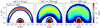 |
Fig. 1. Snapshots of the velocity distribution of the simulations with ne/n0 = 10%. The distributions are obtained at t = 0 |


3. Simulation results
In this section we first present the reference solution with ne/n0 = 10%, showing the detailed evolution of electron distribution and energies of the wave fields, as well as the dispersion relation analysis. Simulation results with varying ne/n0 are presented subsequently to study its effect on the amplification of harmonic emissions. Then we compare three cases with ne/n0 = 5%,10%, and 50% to analyze the detailed wave amplification and particle diffusion process. Finally, we examine the resonance conditions of the amplified wave modes to understand their excitation.
3.1. Harmonic ECME driven by horseshoe electrons (with ne/n0 = 10%)
The evolution of the electron distribution for the reference solution is displayed in Fig. 1 and the accompanying animation. Initially, energetic electrons are distributed along the semicircle in velocity space, with a strong positive gradient below the radius. In the middle of the simulation (t = 150  ), significant diffusion of the horseshoe electrons can be seen. This leads to a smoother gradient and fills up the cavity at lower velocities. At the end of the simulation (t = 300
  ), the gradient of the energetic electrons becomes even smoother. Background electrons are diffused slightly toward higher velocities along the perpendicular direction, indicating perpendicular heating or acceleration.
The temporal energy profiles of various wave field components and the decline in kinetic energy of the total electrons (−ΔEk) are plotted in Fig. 2a, normalized to the initial kinetic energy of energetic electrons (Eke0). At about 50  , Ey and Bz start to increase sharply and reach maximum (∼2 × 10⁻²Eke0) about 120
  , with five orders of magnitude above the corresponding noise level. Their temporal evolutions are consistent with each other. The energies of Ex, Ez, and By later rise to a magnitude of 10−4Eke0, while Bx is the weakest component in energy (∼10−5Eke0). The profile of −ΔEk closely follows the increase of the dominant transverse components (Ey and Bz). After 150
  , almost all field components are saturated.
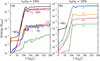 |
Fig. 2. Temporal profiles of panel a: energies of six wave-field components (Ex, Ey, Ez, Bx, By, and ΔBz), panel b: energies of waves in the Z, X2, O1, and X3 modes with ne/n0 = 10%. The energies are normalized to the initial kinetic energy of energetic electrons (Eke0). The dark line refers to the relative decline in the kinetic energy of the electrons. |
Figure 3 presents the distribution of the maximum wave energy in the wave vector k (k∥, k⊥) space over the whole simulation (0–300  ) for Ex, Ey, and Ez. The waves are clearly amplified mainly along the perpendicular direction at |k|∼Ωce/c, 2 Ωce/c, and 3 Ωce/c, respectively. The modes carried by Ey are much stronger than the modes carried by Ex and Ez. This is consistent with the energy profiles plotted in Fig. 2a.
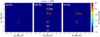 |
Fig. 3. Maximum intensity of (panel a) Ex, (panel b) Ey, and (panel c) Ez in the ω domain in the k∥–k⊥ space as shown by the color map of 20log10[(Ex, Ey, Ez)/(cB0)] over the whole simulation (0–300 |

In Fig. 4 we present the ω-k dispersion diagrams of the perpendicular field components for the mode identification. According to the magnetoionic theory, for perpendicular propagation ( ), the X (and Z) modes are carried by Ex and Ey, and the O mode is carried by Ez. The dispersion curves of the modes are overplotted to facilitate mode identification. The wave modes carried by Ey and Ez are also carried by Bz and By, respectively, according to the Faraday law (k × E = −ωB). According to the ω-k dispersion, in Ey and Bz the Z and X2 modes grow significantly at frequencies of 0.96 Ωce and 1.92 Ωce, respectively, and the X3 mode with ω ∼ 2.9 Ωce manifests a relatively weak growth. The excitation of all the wave modes can be found in a finite frequency range, with a relative bandwidth of ∼5%. For example, the amplification of the Z mode mainly lies in a frequency range of 0.93–0.98 Ωce. Fundamental and harmonic O modes (O1 and O2) are also amplified, but with a much weaker intensity, according to the diagrams of Ez and By. According to the online animation, all modes are amplified within an angular width of 10°–20° centered on the perpendicular direction, as is also indicated by Fig. 3. We note that at 90°, none of the amplified wave modes can be seen in the dispersion diagram of Bx, consistent with the divergence-free condition of B. The growth in energy of Bx comes from the waves propagating at oblique directions (as is shown in the online animation of Fig. 4). The vertical features in panels a, b, and f are artifacts caused by the spectral leakage of the discrete Fourier transform (DFT) analysis.
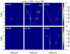 |
Fig. 4. Wave dispersion diagrams of the electric and magnetic components with ne/n0 = 10%, over times 0–300 |

The mode intensities were evaluated by integrating the energies of the corresponding field components within the respective ranges in k space (marked in Fig. 3 with squares) for each time step, based on the Parseval theorem. As illustrated above, Z and X modes are mainly carried by Ex, Ey, and Bz, and O1 is carried by Ez and By. To avoid the contamination of Z mode in Ex, only the Ey and Bz components were considered for the evaluation of the X3 intensity. We note that the X3 energy in Ex is relatively minor. The obtained temporal energy profiles are plotted in Fig. 2b. The energy of the Z mode grows linearly from the beginning of the simulation until its saturation at 110  . The fitted growth rate is about 0.016 Ωce, while the energy conversion rate, that is, the ratio of the mode energy to the initial kinetic energy of energetic electrons, is about 4.1 × 10⁻². Both X2 and X3 start to grow later at 80
  , with growth rates of 0.027 and 0.032 Ωce, respectively, and both end about 110
  . The energy conversion rates of X2 and X3 are 1.7 × 10⁻³ and 5 × 10⁻⁵, respectively. The O1 growth rate is similar to that of the Z mode, and its energy conversion rate is about 5 × 10⁻⁴. The corresponding energies of O2 and O3 in the Ez and By components are lower than those of the X2 and X3 modes by about three orders of magnitude (not shown).
In summary, the horseshoe electrons with ne/n0 = 10% can drive significant cyclotron maser instability, generating waves mainly in Z and X2 modes at frequencies slightly lower than Ωce and 2 Ωce, respectively, in the perpendicular direction. The growths of O1 and X3 modes are relatively weaker. We conclude that the horseshoe-driven maser emission is mainly in the X2 mode for the present case with ne/n0 = 10%.
3.2. Effect of ne/n0 on wave excitations
During solar flares, a bulk energization of electrons may take place, producing an extremely large number of energetic electrons (Aschwanden 2002). The abundance of the energetic electrons (ne/n0) varies from event to event and from stage to stage of a single event. To explore its effect on wave excitations, we varied ne/n0 from 1% to 50% while the other parameters were fixed.
We start with detailed comparisons of the cases with ne/n0 = 5%,10%, and 50%. As displayed in Figs. 1 and 5 as well as in the accompanying animations, the electron diffusion becomes more efficient with more abundant energetic electrons. With ne/n0 = 5%, the diffusion is relatively slow with a large gap even after saturation; with ne/n0 = 10%, the gap is mostly filled up at the end of the simulation; and with ne/n0 = 50%, the hole is entirely filled up before 100  , and the overall shape of distribution becomes similar to the Dory-Guest-Harri distribution (Dory et al. 1965). In this case, background electrons are accelerated considerably in the perpendicular direction, with a significant diffusion toward higher v⊥ in the velocity space.
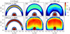 |
Fig. 5. Snapshots of the velocity distribution of the simulations with ne/n0 = 5% (a)–(c) and 50% (d)–(f). The distributions are obtained at t = 0 |


The linear stages for the three cases are (50–150  ), (40–110
  ), and (20–60
  ), indicating that more energetic electrons correspond to a faster evolution (Figs. 2 and 6). For all cases with different ne/n0, 2–5% of Eke0 can be converted into the wave energy, with Ey and Bz being dominant with a similar evolutionary trend. The energies of Ez, By, and Bx increase with increasing ne/n0. In the case of ne/n0 = 50%, the energy evolution of Ex shows an obvious decline after the saturation that is likely due to the damping of the corresponding Z mode.
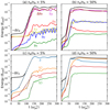 |
Fig. 6. Panels a–b: Temporal profiles of energies of six wave-field components (Ex, Ey, Ez, Bx, By, and ΔBz) with ne/n0 = 5% and 50%. Panels c–b: Temporal energy profiles of the Z, X2, O1, and X3 modes. The energies are normalized to the respective initial kinetic energy of energetic electrons (Eke0). The dark line refers to the relative decline in the kinetic energy of the electrons. |
The intensity maps in the k space are similar for the three cases, with significant perpendicular growth at |k|∼Ωce/c, 2 Ωce/c, and 3 Ωce/c (see Figs. 3 and 7). With a higher density ratio, all the amplified modes become more intense in a broader range of k. Wave growths in Ex and Ez are negligible for ne/n0 = 5% and 10%, while the Ez intensity at |k|∼Ωce becomes very high with ne/n0 = 50%, indicating a significant amplification of O1-mode waves. In Fig. 8 we display the ω-k dispersion analyses in Ey (panels c, e, and h) with θkB = 90°, highlighting the amplified wave modes of Z, X2, and X3. We would like to point out that with ne/n0 = 50%, the wave growth in Ey occurs in a wide range of k at frequencies close to the Z mode, known as the relativistic mode (marked “R”), according to the earlier linear analysis by Pritchett (1984).
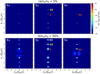 |
Fig. 7. Maximum intensity of (Ex, Ey, Ez) in the ω domain in the k∥-k⊥ space as shown by the color map of 20log10[(Ex, Ey, Ez)/(cB0)] for the whole simulation (0–300 |

Energy profiles of various wave modes are shown in Figs. 2b and 6c–d. They are quite similar to those of the field components. When ne/n0 increases from 5% to 50%, the energy conversion rate of Z mode decreases from ∼5 × 10⁻² to ∼4 × 10⁻³, while the amplification of X2 becomes more efficient: its energy conversion rate increases from ∼6 × 10⁻⁴ to ∼2 × 10⁻². The energy conversion rates of O1 and X3 are lower than those of the Z and X2 modes, which also increase with ne/n0. With ne/n0 = 50%, X2 becomes the most intense mode at the saturation stage, while the Z-mode energy declines with time, likely due to its damping with time, as mentioned above.
Fourier and energy analyses of various modes for cases with ne/n0= 1%, 2.5%, 5%, 7.5%, 10%, 25%, 40%, and 50% are plotted in Fig. 8 for the Eyω-k dispersion and in Fig. 9 for profiles of mode energies and normalized growth rates. The Z, X2, and X3-mode waves become more intense with higher ne/n0 and increasing kinetic energies of energetic electrons. In addition, the R mode appears with ne/n0 higher than 10%.
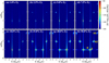 |
Fig. 8. ω-k dispersion diagrams of the pure transverse electric component (Ey) in the perpendicular direction. Each panel represents the result of the simulation with a certain ne/n0. The analyses are performed for the whole stage of each simulation case, which is 0–500 |


The fitted growth rates (in unit of Ωce) with varying density ratios are plotted in Fig. 9a. With increasing ne/n0 from 1% to 50%, all relevant modes (Z, X2, X3, and O1) present a faster evolution with higher growth rates. However, the growth rates are not proportional to the density ratio, as expected, while the increase in growth rate becomes slower with higher density ratio. The energy conversion rate of the Z mode decreases gradually, while those of the other modes (X2, X3, and O1) first increase to maximum values of 4 × 10⁻², 2 × 10⁻⁴, and 3 × 10⁻³Eke0, respectively, and then decline in general (Fig. 9b). It should be noted that the energy conversion rates shown here are the ratios of the mode energy to the kinetic energy of energetic electrons, representing the efficiency of the wave amplification for each case, rather than the obtained wave intensity.
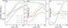 |
Fig. 9. Variation in panel a: fitted linear growth rate (in unit of Ωce), panel b: final energy conversion rate of the Z, X2, X3, and O1 modes with ne/n0. Panel c: ratio of the energy of the O modes and Z/X modes at certain harmonics (EO1/EZ, EO2/EX2, and EO3/EX3) vs. ne/n0. |
As shown in Fig. 9a and b, the energy conversion rates are not directly correlated with the growth rates for different modes. For example, with ne/n0 = 10%, X3 has the highest growth rate but the lowest energy conversion rate, while the Z mode has the highest energy conversion rate with a low value of the growth rate. Similar results have been obtained by Yoon & Ziebell (1995) with a quasi-linear analysis of the cyclotron maser instability of loss-cone electrons. In their results, all the modes grow with an initial energy of 1.0 × 10⁻⁴Eke0, and the Z mode eventually dominates with a growth rate lower than X1. They explained that the growth rate of X1 is more likely to be affected by the evolution of the electron distribution and can only grow for a short duration, while the growth of the Z mode lasts longer. In our simulation, it is more complicated because the initial energy of the different modes varies greatly. The initial energy of the X3 mode is lower than that of the Z mode by two orders of magnitude, while the durations of growth for the two modes are also different. Additionally, the Z mode can be damped after the saturation stage in specific cases. Thus, the eventual energy conversion rate of different modes cannot be directly predicted with the growth rate.
In Fig. 9c we plot the variation in energy ratios of O1 − Z, O2 − X2, and O3 − X3. The energy ratios of O2 − X2 and O3 − X3 remain lower than 10−2. This means that the obtained second- and third-harmonic emissions are almost in the sense of 100% X-mode polarization. The energy ratio of the O1 − Z mode is ∼10−4 with ne/n0 < 5%, increasing to ∼0.15 with ne/n0 ≥ 25%, indicating a more efficient excitation of O1 with larger ne/n0, consistent with the above analysis.
3.3. Resonance analysis
For a complete understanding of the results, we analyzed the resonance conditions of the amplified wave modes (Z, X2, X3, and O1). The cyclotron resonance condition can be written as
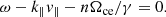
Considering perpendicular wave propagation with k∥ = 0, the condition is simplified as
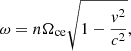
where n is the harmonic number. According to this equation, only waves at frequencies lower than nΩce can be amplified perpendicularly. Therefore the resonance condition cannot be satisfied for the fundamental X mode, whose cutoff frequency is  . The cutoff frequency and resonance frequency of the Z mode are
  and
and  , respectively. Therefore the Z mode and harmonics of the X mode (e.g., X2 and X3) can be amplified. The resonance curves of the three modes are plotted in Fig. 1a with ω = 0.96 Ωce (n = 1), ω = 1.92 Ωce (n = 2), and ω = 2.88 Ωce (n = 3). The corresponding resonance curves overlap with each other and lie in a region with a significant positive gradient of the horseshoe distribution. The wave excitations of these modes are therefore attributed to the shell component of the horseshoe distribution, rather than to the loss-cone component, which occupies only a rather limited region. The frequency of the amplified O1-mode waves are the same as that of the Z mode, corresponding to the same resonance curve.
4. Conclusion and discussion
We investigated the ECME driven by energetic electrons of the horseshoe distribution with ωpe/Ωce = 0.1, appropriate for some solar flares occurring in the strongly magnetized solar atmosphere. In the case with ne/n0 = 10%, both Z and X2-mode waves are amplified efficiently, with minor growth of O1 and X3. The energies of the Z and X2 modes can reach up to 4.1 × 10⁻² and 1.7 × 10⁻³Eke0, respectively, and the X3 energy is lower by two to three orders of magnitude, while the O1 mode is weaker than the X2 mode by 1 order of magnitude in energy. According to the parameter study of the effect of ne/n0, the energy convention rates of X2, X3, and O1 modes first increase to maximum values of 4 × 10⁻², 2 × 10⁻⁴, and 3 × 10⁻³, respectively, and then decline in general. The study shows that the second-harmonic emissions can be directly and efficiently excited through the horseshoe ECME, with ne/n0 ranging from 5% to 50%. This provides a solution to the escaping difficulty of the ECME theory when applied to solar radio spikes, and a possible interpretation of the harmonic structures of solar spikes.
The brightness temperature (TB) of the obtained X2 emission for ne/n0 = 10% can be roughly estimated as follows (Winglee & Dulk 1986b):
![$$ \begin{aligned} K T_\mathrm{B} = \eta ^{1/2} n_\mathrm{e} m_\mathrm{e} v_0^2 V_\mathrm{c} ,\ V_\mathrm{c} = \left[ \left(\frac{\omega }{2\pi c}\right)^3\frac{\Delta \omega }{\omega } 2\pi \Delta \theta \sin \theta \right]^{-1}, \end{aligned} $$](/articles/aa/full_html/2021/07/aa40427-21/aa40427-21-eq42.gif)
where Vc is the coherence volume, η is the fraction of the energy of energetic electrons converted into X2 emission, and  is the average kinetic energy of energetic electrons. According to our result, η = 0.0017,
  mec2, Δω/ω ≈ 0.05, θ = 90°, and Δθ = 10°. Assuming the number density of the background (energetic) electrons to be n0 = 109 cm−3 (ne = 108 cm−3), the corresponding plasma frequency is ∼285 MHz, and the fundamental electron cyclotron frequency is fce ≈ 2.85 GHz. The frequency of the obtained X2 emission f is 1.92 fce (≈5.5 GHz.) The simulation lasts for only ∼1 μs. If the temporal resolution of radio observation is ∼1 ms and assuming the filling factor of radio sources is 10−2 or 10−3, then the obtained TB is ∼1012 K, comparable with observations. Considering that second-harmonic emissions might be partly absorbed by the third-harmonic layer, TB can be lower. According to our investigation, with higher ne/n0, the X2 mode reaches a higher level of energy, corresponding to larger TB. The obtained emission is characterized by a high brightness temperature, a short duration, a narrow bandwidth, and 100% X-mode polarization. These characteristics are consistent with the observed features of solar spikes.
With the same assumption, we estimated the brightness temperature of X2 emissions to be 1011 and 1015 K with ne/n0 = 5% and 50%, respectively. These estimates are in line with the observations of solar radio spikes. We would like to point out that bulk acceleration could occur during solar flares, as indicated by HXR observations (Raymond et al. 2012; Benz 2017). This makes it demanding to study wave amplifications in plasmas with ne/n0 ≥ 25%, although energetic electrons with a high proportion could cause an extremely quick response of the ambient plasmas and may not last steadily for seconds. Individual solar radio spikes occur within an extremely short time, however; the durations of each spike are as short as several to some dozen milliseconds.
For solar spikes, harmonic structures are reported in many events. Staehli & Magun (1986) observed the harmonic structure of solar spikes at frequencies of 3.47 and 5.2 GHz, with a frequency ratio of 2:3. Guedel (1990) reported nine events with harmonic structures, with frequency ratios being 2:3, 2:3:4, 3:4, etc. In the most recent study, Feng et al. (2018) reported an event at metric wavelength, with harmonic structures of 2:3:4. Excitations of various harmonics are necessary to interpret the observed multiharmonic structures of solar spikes. In our simulation, simultaneous excitations of X2 and X3 are obtained. The energy of X3 is lower than that of X2 by two to three orders of magnitude, according to our simulation, but the X2 mode may undergo stronger absorption during its escape from the source. Emissions at higher harmonics could not be resolved in our solutions due to the limited grid resolution. Their intensity, if properly resolved, should be even weaker than the third-harmonic emission, according to the linear kinetic theory.
According to the simulation result with ne/n0 = 50%, a significant decline in the energy of the Z mode is present after saturation (Fig. 6d). In this case, the Z mode mainly propagates perpendicularly to the background magnetic field, and the background electrons are heated considerably in the perpendicular direction, as was pointed out in Sect. 3.2. This indicates that the Z mode is damped by the cyclotron-resonant absorption of thermal electrons. The damping could contribute to the heating process of plasmas during solar flares. It is intriguing to further investigate the role of the Z mode in flare heating of coronal plasmas, which can be excited quite efficiently through electron-cyclotron maser instability (see, e.g., White et al. 1986).
It should be noted that our simulations were performed with a uniform-field assumption, driven by the analytically prescribed distribution function of the horseshoe type. In reality, solar radio bursts are a consequence of the multiscale process of solar eruption, involving large-scale eruption, magnetic reconnection, electron acceleration, and further transport. As mentioned in the introduction, Yousefzadeh et al. (2021) performed simulations of energetic electrons traveling along a large-scale coronal loop with the guiding-center method. They fed the obtained velocity distribution function into the PIC system and found efficient excitation of the X2 mode with ωpe/Ωce = 0.25. Further studies along this line of thought with the electron distribution determined in a self-consistent manner should be pursued. In the present study, simulations were performed with ωpe/Ωce = 0.1, representing the plasma condition in the flare regions with very strong magnetic field. Régnier (2015) estimated the ωpe/Ωce ratio in the solar corona by combining the force-free field extrapolation and hydrostatic models, and found that similarly low values of ωpe/Ωce exist in the corona for active regions with a complex magnetic topology. Nevertheless, future studies should consider the effect of ωpe/Ωce. Other features such as the energy of horseshoe electrons and types of velocity distributions should also be evaluated.
Movies
Movie 1 associated with Fig. 1 (fig1_animation) Access here
Movie 2 associated with Fig. 4 (fig4_animation) Access here
Movie 3 associated with Fig. 5 (fig5_animation) Access here
Acknowledgments
This study is supported by the National Natural Science Foundation of China (11790303 (11790300), 11750110424, and 11873036). The authors acknowledge the Beijing Super Cloud Computing Center (BSC-C, URL: http://www.blsc.cn/) for providing HPC resources, and the open-source Vector-PIC (VPIC) code provided by Los Alamos National Labs (LANL). The authors thank Dr. Bing Wang (Shandong University) for helpful discussion.
References
- Aschwanden, M. J. 1990, A&AS, 85, 1141 [NASA ADS] [Google Scholar]
- Aschwanden, M. J. 2002, Space Sci. Rev., 101, 1 [Google Scholar]
- Aschwanden, M. J., Benz, A. O., & Kane, S. R. 1990, A&A, 229, 206 [NASA ADS] [Google Scholar]
- Benz, A. O. 1985, Sol. Phys., 96, 357 [NASA ADS] [CrossRef] [Google Scholar]
- Benz, A. O. 1986, Sol. Phys., 104, 99 [NASA ADS] [CrossRef] [Google Scholar]
- Benz, A. O. 2017, Liv. Rev. Sol. Phys., 14, 2 [Google Scholar]
- Bowers, K. J., Albright, B. J., Yin, L., Bergen, B., & Kwan, T. J. T. 2008, Phys. Plasmas, 15, 055703 [NASA ADS] [CrossRef] [Google Scholar]
- Bowers, K. J., Albright, B. J., & Yin, L. 2009, J. Phys. Conf. Ser., 180, 012055 [CrossRef] [Google Scholar]
- Chernov, G. P. 2011, Fine Structure of Solar Radio Bursts, 375 [CrossRef] [Google Scholar]
- Dory, R. A., Guest, G. E., & Harris, E. G. 1965, Phys. Rev. Lett., 14, 131 [NASA ADS] [CrossRef] [Google Scholar]
- Droege, F. 1977, A&A, 57, 285 [NASA ADS] [Google Scholar]
- Ergun, R. E., Carlson, C. W., McFadden, J. P., et al. 2000, ApJ, 538, 456 [NASA ADS] [CrossRef] [Google Scholar]
- Feng, S. W. 2019, Ap&SS, 364, 4 [CrossRef] [Google Scholar]
- Feng, S. W., Chen, Y., Li, C. Y., et al. 2018, Sol. Phys., 293, 39 [CrossRef] [Google Scholar]
- Fleishman, G. D., & Mel’nikov, V. F. 1998, Phys. Usp., 41, 1157 [NASA ADS] [CrossRef] [Google Scholar]
- Guangs Li, H. 1987, Sol. Phys., 114, 363 [NASA ADS] [CrossRef] [Google Scholar]
- Guedel, M. 1990, A&A, 239, L1 [Google Scholar]
- Guedel, M., Benz, A. O., & Aschwanden, M. J. 1991, A&A, 251, 285 [Google Scholar]
- Holman, G. D., Eichler, D., & Kundu, M. R. 1980, in Radio Physics of the Sun, eds. M. R. Kundu, & T. E. Gergely, 86, 457 [CrossRef] [Google Scholar]
- Huang, G., & Nakajima, H. 2005, Ap&SS, 295, 423 [CrossRef] [Google Scholar]
- Marder, B. 1987, J. Comput. Phys., 68, 48 [NASA ADS] [CrossRef] [Google Scholar]
- McKean, M. E., Winglee, R. M., & Dulk, G. A. 1989, Sol. Phys., 122, 53 [CrossRef] [Google Scholar]
- Melrose, D. B. 2017, Rev. Mod. Plasma Phys., 1, 5 [CrossRef] [Google Scholar]
- Melrose, D. B., & Dulk, G. A. 1982, ApJ, 259, 844 [NASA ADS] [CrossRef] [Google Scholar]
- Melrose, D. B., & Wheatland, M. S. 2016, Sol. Phys., 291, 3637 [CrossRef] [Google Scholar]
- Pritchett, P. L. 1984, J. Geophys. Res., 89, 8957 [NASA ADS] [CrossRef] [Google Scholar]
- Pritchett, P. L., Strangeway, R. J., Ergun, R. E., & Carlson, C. W. 2002, J. Geophys. Res. (Space Phys.), 107, 1437 [CrossRef] [Google Scholar]
- Raymond, J. C., Krucker, S., Lin, R. P., & Petrosian, V. 2012, Space Sci. Rev., 173, 197 [NASA ADS] [CrossRef] [Google Scholar]
- Régnier, S. 2015, A&A, 581, A9 [NASA ADS] [CrossRef] [EDP Sciences] [Google Scholar]
- Robinson, P. A. 1989, ApJ, 341, L99 [CrossRef] [Google Scholar]
- Sharma, R. R., & Vlahos, L. 1984, ApJ, 280, 405 [NASA ADS] [CrossRef] [Google Scholar]
- Sharma, R. R., Vlahos, L., & Papadopoulos, K. 1982, A&A, 112, 377 [NASA ADS] [Google Scholar]
- Slottje, C. 1978, Nature, 275, 520 [NASA ADS] [CrossRef] [Google Scholar]
- Staehli, M., & Magun, A. 1986, Sol. Phys., 104, 117 [NASA ADS] [CrossRef] [Google Scholar]
- Tarnstrom, G. L., & Philip, K. W. 1972, A&A, 16, 21 [Google Scholar]
- Treumann, R. A. 2006, A&ARv, 13, 229 [NASA ADS] [CrossRef] [Google Scholar]
- Twiss, R. Q. 1958, Aust. J. Phys., 11, 564 [NASA ADS] [CrossRef] [Google Scholar]
- Vlahos, L. 1987, Sol. Phys., 111, 155 [CrossRef] [Google Scholar]
- White, S. M., Melrose, D. B., & Dulk, G. A. 1986, Adv. Space Res., 6, 163 [CrossRef] [Google Scholar]
- White, S. M., Benz, A. O., Christe, S., et al. 2011, Space Sci. Rev., 159, 225 [NASA ADS] [CrossRef] [Google Scholar]
- Winglee, R. M., & Dulk, G. A. 1986a, Sol. Phys., 104, 93 [NASA ADS] [CrossRef] [Google Scholar]
- Winglee, R. M., & Dulk, G. A. 1986b, ApJ, 307, 808 [Google Scholar]
- Wu, C. S. 1985, Space Sci. Rev., 41, 215 [NASA ADS] [CrossRef] [Google Scholar]
- Wu, C. S., & Lee, L. C. 1979, ApJ, 230, 621 [NASA ADS] [CrossRef] [Google Scholar]
- Wu, C. S., & Freund, H. P. 1984, Radio Sci., 19, 519 [CrossRef] [Google Scholar]
- Wu, D. J., Chen, L., Zhao, G. Q., & Tang, J. F. 2014, A&A, 566, A138 [CrossRef] [EDP Sciences] [Google Scholar]
- Yoon, P. H., & Ziebell, L. F. 1995, Phys. Rev. E, 51, 4908 [CrossRef] [Google Scholar]
- Yoon, P. H., Weatherwax, A. T., & Rosenberg, T. J. 1998, J. Geophys. Res., 103, 4071 [NASA ADS] [CrossRef] [Google Scholar]
- Yousefzadeh, M., Ning, H., & Chen, Y. 2021, ApJ, 909, 3 [CrossRef] [Google Scholar]
All Figures
|
Fig. 1. Snapshots of the velocity distribution of the simulations with ne/n0 = 10%. The distributions are obtained at t = 0 |
| In the text | |
|
Fig. 2. Temporal profiles of panel a: energies of six wave-field components (Ex, Ey, Ez, Bx, By, and ΔBz), panel b: energies of waves in the Z, X2, O1, and X3 modes with ne/n0 = 10%. The energies are normalized to the initial kinetic energy of energetic electrons (Eke0). The dark line refers to the relative decline in the kinetic energy of the electrons. |
| In the text | |
|
Fig. 3. Maximum intensity of (panel a) Ex, (panel b) Ey, and (panel c) Ez in the ω domain in the k∥–k⊥ space as shown by the color map of 20log10[(Ex, Ey, Ez)/(cB0)] over the whole simulation (0–300 |
| In the text | |
|
Fig. 4. Wave dispersion diagrams of the electric and magnetic components with ne/n0 = 10%, over times 0–300 |
| In the text | |
|
Fig. 5. Snapshots of the velocity distribution of the simulations with ne/n0 = 5% (a)–(c) and 50% (d)–(f). The distributions are obtained at t = 0 |
| In the text | |
|
Fig. 6. Panels a–b: Temporal profiles of energies of six wave-field components (Ex, Ey, Ez, Bx, By, and ΔBz) with ne/n0 = 5% and 50%. Panels c–b: Temporal energy profiles of the Z, X2, O1, and X3 modes. The energies are normalized to the respective initial kinetic energy of energetic electrons (Eke0). The dark line refers to the relative decline in the kinetic energy of the electrons. |
| In the text | |
|
Fig. 7. Maximum intensity of (Ex, Ey, Ez) in the ω domain in the k∥-k⊥ space as shown by the color map of 20log10[(Ex, Ey, Ez)/(cB0)] for the whole simulation (0–300 |
| In the text | |
|
Fig. 8. ω-k dispersion diagrams of the pure transverse electric component (Ey) in the perpendicular direction. Each panel represents the result of the simulation with a certain ne/n0. The analyses are performed for the whole stage of each simulation case, which is 0–500 |
| In the text | |
|
Fig. 9. Variation in panel a: fitted linear growth rate (in unit of Ωce), panel b: final energy conversion rate of the Z, X2, X3, and O1 modes with ne/n0. Panel c: ratio of the energy of the O modes and Z/X modes at certain harmonics (EO1/EZ, EO2/EX2, and EO3/EX3) vs. ne/n0. |
| In the text | |
Current usage metrics show cumulative count of Article Views (full-text article views including HTML views, PDF and ePub downloads, according to the available data) and Abstracts Views on Vision4Press platform.
Data correspond to usage on the plateform after 2015. The current usage metrics is available 48-96 hours after online publication and is updated daily on week days.
Initial download of the metrics may take a while.