| Issue |
A&A
Volume 651, July 2021
|
|
|---|---|---|
| Article Number | A63 | |
| Number of page(s) | 12 | |
| Section | Numerical methods and codes | |
| DOI | https://doi.org/10.1051/0004-6361/202040119 | |
| Published online | 13 July 2021 | |
Multi-dimensional population modelling using frbpoppy: Magnetars can produce the observed fast radio burst sky
1
ASTRON – the Netherlands Institute for Radio Astronomy, Oude Hoogeveensedijk 4, 7991 PD Dwingeloo, The Netherlands
e-mail: This email address is being protected from spambots. You need JavaScript enabled to view it.
2
Anton Pannekoek Institute for Astronomy, University of Amsterdam, Science Park 904, 1098 XH Amsterdam, The Netherlands
Received:
11
December
2020
Accepted:
21
April
2021
Abstract
Fast radio bursts (FRBs) are energetic, short, bright transients that occur frequently over the entire radio sky. The observational challenges following from their fleeting, generally one-off nature have prevented the identification of the underlying sources producing the bursts. As the population of detected FRBs grows, the observed distributions of brightness, pulse width, and dispersion measure now begin to take shape. Meaningful direct interpretation of these distributions is, however, made impossible by the selection effects that telescope and search pipelines invariably imprint on each FRB survey. Here, we show that multi-dimensional FRB population synthesis can find a single, self-consistent population of FRB sources that can reproduce the real-life results of the major ongoing FRB surveys. This means that individual observed distributions can now be combined to derive the properties of the intrinsic FRB source population. The characteristics of our best-fit model for one-off FRBs agree with a population of magnetars. We extrapolated this model and predicted the number of FRBs future surveys will find. For surveys that have commenced, the method we present here can already determine the composition of the FRB source class, and potentially even its subpopulations.
Key words: radio continuum: general / methods: statistical
© ESO 2021
1. Introduction
Fast radio bursts (FRBs) are bright millisecond-duration radio transients of unknown origin (see Petroff et al. 2019; Cordes & Chatterjee 2019). Recent observations of SGR 1935+2154 suggest that some FRBs can be associated with magnetars (Bochenek et al. 2020; CHIME/FRB Collaboration 2020). Despite these detections, much is still unknown about the intrinsic FRB source population. The number density function could be fairly flat (Lawrence et al. 2017) or quite steep (James et al. 2019). The luminosity function could be described by a power-law distribution (Caleb et al. 2016) or a Schechter function (Luo et al. 2018; Fialkov et al. 2018). The difference in intrinsic pulse width distribution of repeating and one-off FRB sources could be due to an intrinsic difference (CHIME/FRB Collaboration 2019; Fonseca et al. 2020; Cui et al. 2021) or due to selection effects (Connor et al. 2020).
In recent years, a number of observatories have focussed on detecting larger numbers of FRBs and studying these in more detail to help solve some of the open questions listed above. These telescopes and surveys include the Australian Square Kilometre Array Pathfinder (ASKAP; Macquart et al. 2010; Johnston et al. 2007), the FRB survey on Canadian Hydrogen Intensity Mapping Experiment (CHIME/FRB; CHIME/FRB Collaboration 2018), and the Apertif survey at Westerbork (Maan & van Leeuwen 2017; van Leeuwen et al., in prep.). By now, over a hundred FRB detections have been made (Petroff & Yaron 2020). This order of magnitude increase in detected FRBs provides a unique opportunity to conduct population studies.
Prior FRB population studies have focussed on different aspects, such as Caleb et al. (2016), who conducted one of the first population studies, investigating whether FRB sources could be considered to have a cosmological, high-redshift origin. Just a selection of these show papers focussed on pulse broadening (Qiu et al. 2020), spectral properties (Macquart et al. 2019), source count distributions (James et al. 2019), fluence and dispersion measure distributions (Lu & Piro 2019), or a mix of properties from scattering to pulse width (Bhattacharya & Kumar 2020). Few of these earlier studies incorporate all three aspects we consider important when conducting a full-scale population study: selection effects, describing detections from multiple surveys, and making the code available. Extrapolating from observations to the properties of an intrinsic population is difficult without taking the full range of selection effects for different surveys into account.
Population synthesis offers the unique opportunity to probe an intrinsic source population through extensive modelling. By simulating an intrinsic source population and convolving this population with a model of selection effects, a simulated observation can be made. Comparing this modelled observation to real observations provides a means to evaluate the simulated intrinsic population. The better the simulated observed population fits real observations, the more likely the simulated intrinsic population is to be an accurate descriptor of the real intrinsic population. This method has been applied successfully, and extensively, in a wide range of fields: from pulsars (Taylor & Manchester 1977) to high-mass binaries (Portegies Zwart & Verbunt 1996), from gamma ray bursts (Ghirlanda et al. 2013) to stellar evolution (Izzard & Halabi 2018).
In this paper, we aim to determine which physical birth and emission properties best describe the intrinsic one-off FRB population. We do this through a large scale FRB population synthesis, exploring an eleven-dimensional parameter space through Monte Carlo simulations.
This paper comprises the following sections. Firstly, our methods are described in Sect. 2. Secondly, our results can be found in Sect. 3, which is split into three parts. We start by showing the effect of various intrinsic parameters on a log N − log S distribution. We then show the results of a Monte Carlo simulation through which we derive the optimal intrinsic parameters with which the observed one-off FRB population can be described. We subsequently used these optimal parameters to predict expected detections by future radio transient surveys. Thirdly, a discussion of the results can be found in Sect. 4, and lastly, our conclusions are presented in Sect. 5.
2. Methods
One way to probe an intrinsic source population is through population synthesis. An advantage of population synthesis is that it takes into account both the physics of the underlying population and selection effects. Synthesising populations requires an intrinsic source population to be modelled before convolving it with a range of selection effects to obtain an observed population. Comparing such a population to real observed populations subsequently allows various intrinsic source population parameters to be evaluated and determined. The better the simulation, the better the inputs are able to describe the true intrinsic population.
In Gardenier et al. (2019), we presented v1.0 of frbpoppy, an open source code package capable of FRB population synthesis in Python. We subsequently expanded its functionality to include the modelling of repeating FRB sources in v2.0 of frbpoppy (Gardenier et al. 2021). We build on this prior work in this paper, and we accordingly published the code used for these results in v2.1 of frbpoppy1.
In this paper, we aim to provide a method by which intrinsic FRB source population parameters can be derived. We do so by adopting an iterative approach to population synthesis, using the outcome of a simulation to determine the choice of input parameters for subsequent runs. This allows for the properties of an intrinsic source population that best describe current observations to be derived.
We used v2.0 of frbpoppy to model our intrinsic populations, surveys, and observed populations. Modelling these components requires various parameters as input. For the modelling of intrinsic populations, we adopted the parameters given in Table 1, and for surveys we adopted the parameters given in Table 2. A number of these parameters may require further explanation. Specifically, in frbpoppy, the luminosity of a burst refers to the isotropic equivalent bolometric luminosity in the radio, where the frequency range is defined by νlow, high. When drawing such luminosities from a power law, we define a power law to follow N(L) ∝ Lli with luminosity index li. Additionally, log-normal distributions in frbpoppy use the desired mean and standard deviation given as input to calculate the mean and standard of the natural logarithm of said variables. These values subsequently allow a log-normal distribution to be drawn around the desired mean and with the desired spread. For additional information on the modelling process or the parameter inputs, we refer the reader to Gardenier et al. (2019, 2021).
Parameters and values used to model intrinsic FRB populations in this paper.
Overview of the parameters adopted for the simulation of surveys.
In this first Monte Carlo frbpoppy paper, we limited ourselves to one-off FRB sources. While including the repeating population could provide stronger constraints on the intrinsic FRB population, modelling repeater populations would require exponentially more compute resources. We discuss the implications of this approach in Sect. 4.2.2.
2.1. Log N–Log S
A log N − log S distribution shows the number of detections of sources above a limiting signal-to-noise (S/N) threshold. We note that we use log N − log S to refer to the cumulative distribution of the number of detected FRBs greater than a limiting S/N. While this relates to a similar distribution for peak flux density, or indeed fluence, a limiting S/N has the advantage of incorporating all survey selection effects without attempting to account for them. This allows surveys to be compared according to the same metric.
We chose to model such distributions to show the effect of various intrinsic parameters on an observed distribution. All such simulations start with a simple population (see Table 1), intended to model a population with the most basic assumptions. From this simple population, we modelled populations with varying maximum redshifts zmax. To investigate the effect of different luminosity functions, we additionally generated populations with power laws containing different slopes – all within the range of 1040 − 1043 ergs s−1. We also simulated populations with different values of the spectral index si, from −2 to 2. Finally, we also investigated the effect of various pulse width models by simulating populations with a value of 10 ms, a normal distribution of values with a mean of 10 ms and standard deviation of 10 ms and lastly a log-normal distribution with an underlying mean of 10 ms and 10 ms.
The difficulty in drawing meaningful conclusions from a one-dimensional view such as the log N − log S distribution, described in more detail Sect. 4.1, shows the need for a multi-dimensional approach.
2.2. Monte Carlo
By conducting a Monte Carlo simulation, we aim to derive properties of the intrinsic FRB population. Exploring all possible combinations of the parameter space in frbpoppy would be impractical due to the sheer number of inputs and the computational constraints. Instead, we chose subsets of parameters, over which we iterated, before shifting to a next set. To ensure our results’ convergence towards a global maximum, we performed additional runs in which we returned to prior parameters sets. Better fits within that parameter space indicate that a better global fit has been found. That is in essence what a Monte Carlo simulation is – a method in which more runs lead to a better result. In our case, a better result is when a simulation provides a more accurate representation of an observed population than a previous simulation. We chose to measure our success in terms of a total goodness of fit (GoF). To avoid optimising towards a local maximum, we evaluated each simulation on multiple areas.
We assigned three goodness of fit estimators to each simulated population, reflecting their measure of success. The first is the p-value corresponding to a two-sample Kolmogorov–Smirnov (KS) test applied to the simulated and corresponding real dispersion measure (DM) distribution. This real distribution is obtained by using the frbcat package (Gardenier 2020) to access the FRB catalogue hosted on the Transient Name Server (TNS; Petroff & Yaron 2020). We chose to filter out any repeating FRB sources to avoid adding significant weight to their observed parameters. By grouping the database by survey, we allowed a separate DM and S/N distribution to be derived for each survey. The results in this paper are based on the TNS catalogue as available on 2 October 2020. The second goodness of fit was derived in a similar fashion to the first value, but instead for the corresponding S/N distributions. The third goodness of fit is a weighting factor based on how well a simulation matches the observed FRB rate. We stared by calculating our rate as
 (1)
(1)
with rate r, number of detected FRBs nfrbs, and number of days ndays. To avoid the simulation size affecting the results, we chose to normalise all rates by the rate obtained with the htru survey (Keith et al. 2010) using the same inputs. This turns our weighting function into
 (2)
(2)
with the weight w, survey rate rsurvey and HTRU rate rhtru. Here, rate ratios are determined both for simulated detections (sim) and real detections (real). As the TNS catalogue does not include the length of time spent observing, we use rates available in literature to obtain a real rate per survey. These values can be found in Table 3.
FRB detection rates for various surveys.
To limit compute requirements we chose to model FRBs out to a maximum redshift of zmax = 1. Almost all FRBs in our initial observed sample have an implied redshift below 1. For non-localised FRBs, the redshift is only inferred from the measured DM. To ensure we compare only measured parameters, not inferred ones, we limit our evaluation of both real and simulated populations to bursts with a DMtot ≤ 950, not redshift zmax = 1. That way, any selection effects apply equally to both sets. Only four real FRBs were detected above the threshold, and they were cut. We discuss the implications of this choice in Sect. 4.2.
For each intrinsic population, we simulated the surveying of several surveys. We chose to use four surveys to constrain the intrinsic FRB population: Parkes-HTRU, CHIME-FRB, ASKAP-Incoh, and WSRT-Apertif. These four surveys cover most of the one-off FRB detections to date (see the Transient Name Server; Petroff & Yaron 2020), and so they provide a solid basis from which to establish the properties of the intrinsic FRB population.
Our aim is to derive an optimum set of values for each set of intrinsic population parameters being evaluated. We started by generating populations with complex inputs, shown in Gardenier et al. (2019) to be able to replicate Parkes-HTRU and ASKAP-Fly rates. We then calculated a single global GoF for each combination of values being evaluated by taking the weighted median of all GoFs of populations modelled with the same input. We chose to use this median as it damps the effect of outliers. By including weights, we additionally allowed the GoF to reflect how well relative rates were simulated. Within this newly constructed GoF space, the inputs that produce the highest GoF were marked as optimum. To gain an understanding of the underlying space, we visually inspected sample runs. This allowed us to, for example, avoid adding noise by including mostly featureless parameter spaces. An example of this can be seen in Fig. 1, in which two GoF spaces over different parameters are visualised. Most parameter spaces contain regions with clearly elevated GoF values (as seen in the left panel of Fig. 1). For those, we use the optimum GoF values for the subsequent run. In contrast, other parameter spaces, such as the one seen in the right panel of Fig. 1, are quite featureless. These teach us that the underlying parameters have little direct influence on the observed population. We only evaluated these spaces in the first run. We found that when including such spaces in subsequent runs, the somewhat random location of the exact optima added significant noise to the results. After running through several parameter sets, we restarted the cycle until we converged on a global optimum.
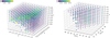 |
Fig. 1. Goodness-of-fit (GoF) spaces spanned by two different sets of parameters. Higher GoFs are denoted both in brighter colours and larger markers. Left panel: an example is seen of a clear optimal region of a parameter space. In comparison to the right panel, this shows a parameter space with no clear optimal region. Each marker represents the weighted median GoF reflecting the results of multiple surveys in multiple dimensions. |
3. Results
In this section, we present our simulations and outcomes. We discuss their implications in Sect. 4.
3.1. Log N–Log S
One of the main questions driving the field of FRBs is, what creates these bursts? The answer requires an understanding of the conditions in which an FRB can be created. This requires knowledge of the properties of the underlying source population. With hundreds of catalogued FRB detections (Petroff & Yaron 2020), it has become possible to probe this intrinsic source population. Doing so is, however, challenging: firstly because selection effects prohibit a direct one-to-one mapping between observed and intrinsic distributions (see e.g., Connor 2019), and secondly because observed distributions are often a one-dimensional representation of a higher dimensional subspace of an intrinsic source population.
With frbpoppy, we can show how various intrinsic population properties can affect an observed distribution. Such simulations also illustrate the difficulties in reversing the process to determine intrinsic population properties from an observed distribution. An observed log N − log S is a tantalizing distribution from which to infer population properties. Such reasoning is tempting as a deviation from a −3/2 slope expected from Euclidean universe can, for instance, be ascribed to non-Euclidean effects on source counts in ΛCDM. The flattening of a log N − log S distribution could indeed prove an invaluable and unique cosmological probe. Nonetheless, we advise caution in such an interpretation as other intrinsic parameters can provide a similar effect, as shown below.
Figure 2 displays the effects that various intrinsic parameters have on observed log N − log S distributions. Four panels are presented in this figure, each representing a different intrinsic parameter space. Within each panel, we show the effect of varying the intrinsic distribution type on the observed distribution. Differing line styles denote the cosmological effects on these variations, ensuring that both a simple, local, Euclidean populations, and populations out to high redshifts are represented. The details of these populations can be found in Sect. 2.1. To help guide the eye, we plot −3/2 slopes with thin grey lines as a reference. As all simulations were run with a perfect survey, with, by definition, an arbitrary S/N threshold, we chose to normalise all S/N values to a minimum value of 1 (i.e. left alignment of the distributions), allowing for a clean comparison between various trends.
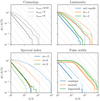 |
Fig. 2. Cumulative distribution of the number of detected FRBs greater than a limiting S/N. Each panel shows the effect on the detected S/N from three different inputs for the parameter denoted above the panel. Each panel additionally shows the cosmological effect on the various input distributions, denoted by the line styles given in the top left plot. Simulated observed S/N distributions can be seen for intrinsic source populations spanning various redshifts (top left), various intrinsic luminosity distributions (top right), various spectral indices (bottom left), and various intrinsic pulse-width distributions (bottom right). We note that considering the arbitrary nature of a S/N threshold for a perfect survey, all distributions were normalised to a S/N of one (i.e. the distributions are left aligned). This allows for a cleaner comparison between trends. Each panel additionally features thin grey Euclidean lines with a slope of −3/2, such that various distributions can easily be compared. |
The diverse effects seen in Fig. 2 serve as an aid for those trying to couple theory to observational expectations and the inverse. For us, the similarity between distributions shows the clear need for a multi-dimensional approach to properly investigate the intrinsic FRB source population.
3.2. Monte Carlo
Much remains unknown about the properties of the intrinsic FRB population (see Petroff et al. 2019; Cordes & Chatterjee 2019). Monte Carlo simulations allow us to build a coherent picture of this population by exploring how reasonable different areas of the source parameter space are. Rather than trying to invert the observed parameter space, which is biased and incomplete, population synthesis attempts to recreate the full underlying picture. We look at many hypothetical underlying FRB populations through the lens of each survey, and investigate which view best matches the actually detected burst set.
In Fig. 3, we show the results of our Monte Carlo simulations. We split our global parameter space into subsets and loop over them to avoid the sixty-day computational cost of directly searching the complete eleven-dimensional space. Each panel individually shows the weighted median distribution of GoFs for each run. These GoFs reflect how well our simulated observations match real observations of a variety of surveys. Additionally, each run shows the location of the maximum GoF within that parameter space, indicating which parameter values show the best fit to reality. The optimum values resulting in the best fit across all parameter sets are shown above each panel.
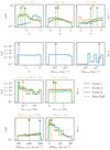 |
Fig. 3. Overview showing how well various intrinsic parameter values can describe current one-off FRB observation, all expressed in a GoF. Each row shows the set of parameters over which was iterated. Each panel shows the result of multiple runs, allowing the convergence to be checked. Each run shows the weighted median of GoFs for each parameter value, with a marker denoting the maximum GoF within that parameter space. From top left to bottom right: log N − log S slope α, spectral index si, luminosity index li, minimum luminosity lummin, maximum luminosity lummax, mean intrinsic pulse width wint, mean, standard deviation intrinsic pulse width wint, std, Macquart index DMIGM, slope, and host dispersion measure DMHost. |
To ensure our fits approach a global rather than a local maximum, we ran additional cycles over all parameters, the results of which are shown in a orange and green. The higher GoF values of a run indicate our Monte Carlo to be converging on a global maximum, with lower values a divergence. This provides a way to check whether subsequent cycles are heading in the right direction.
Various trends are noticeable in these panels, with some showing flatter distributions than others. We found the GoF parameter space of set 2 (the luminosity parameters) to be fairly featureless, which is visible in the right panel of Fig. 1. Test runs showed that subsequent iterations moved the optimum around without statistically significant improvement to the outcome. We thus used the output of set 1 in all subsequent runs and avoided the parameter space for subsequent cycles.
Our complex input model produces simulated FRBs out to redshift zmax = 1 (cf. Sect. 2.2). To ensure our simulation can also describe FRB detections at high DMs (see e.g., Bhandari et al. 2018), which appear to be emitted farther out, we additionally modelled the optimum population to a higher redshift of zmax = 2. We find this population is still equally able to describe the observed DM and S/N distributions and the rates.
We expand on the interpretation of the results for each parameter in Sect. 4.2, and how these compare to predictions in literature. Together, these optimal parameters describe a best-fit intrinsic population (see optimum in Table 1). From this best model, expected FRB rates for future surveys can be derived.
3.3. Future surveys
A large number of new radio observatories are in the construction or design phase: from FAST-CRAFTS (Zhang et al. 2019), to SKA-Low and SKA-Mid (Dewdney et al. 2013), and, for example, PUMA-Full (Castorina et al. 2020) or CHORD (Vanderlinde et al. 2019). We simulated the detections expected for these surveys in comparison to current or past surveys such as Parkes-HTRU or WSRT-Apertif. We derived these results using the optimal population given in Table 1 together with the surveys presented in Table 2. We adopted an Airy beam pattern for all of the surveys, as few have beam pattern information at this stage. This allows for a cleaner comparison between the surveys. Figure 4 displays the dispersion measure and log N − log S distributions expected for these surveys. The associated rates are displayed in the same figure and listed in Table 3. Based on these numbers, we discuss the relative advantages of each survey in Sect. 4.3.
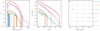 |
Fig. 4. Expected observations of one-off FRBs by current and future surveys. Left: simulated dispersion measure distributions for various surveys. Middle: log N − log S distributions showing the number of detections above a S/N threshold for several surveys. Right: expected rates for each survey based on frbpoppy simulations. All rates have been set such that the simulated Parkes-HTRU rate corresponds to the observed Parkes-HTRU rate. We note that the size of this set of simulated detected Parkes-HTRU FRBs was large enough to produce reliable rates, but not large enough to properly sample the Parkes-HTRU distributions in the left panel. |
4. Discussion
In Sect. 3, we report the distributions and parameters that resulted from our simulations. Here, we discuss which source model fits best with these. We compare our outcomes with predictions by three source models. First, the radio-loud magnetar models, where the bursts are generated as magnetically powered radio flares (e.g., Lu & Kumar 2018, Model I). Second, spin-down-powered models in which bursts are generated as supergiant pulses from young pulsars (e.g., Cordes & Wasserman 2016, Model II). And third, models in which bursts are generated through blast wave masers (e.g., Lyubarsky 2014, Model III). For these three model classes, some quantitative expectations for FRB distributions exist. These follow either from the observed behaviour of similar lower-powered systems, or from theoretical considerations. A number of other highly interesting models, such as those involving pulsar magnetospheres swept back by strong plasma streams (Zhang 2018) or binary neutron-star mergers (Totani 2013) do not yet make predictions we can test against.
4.1. Log N–Log S
In Fig. 2, we show the effect of various intrinsic parameters on observed S/N distributions. The resulting redshifted distributions seen in the top left panel of Fig. 2 are understandable when considering effects arising over cosmological distances. For a limiting redshift of 0.01, only the local universe is probed, resulting in a Euclidean universe where volume grows with V ∝ R3 over radius R. As luminosity L ∝ R−2, the expected cumulative S/N distribution is expected to follow a slope of −3/2. This is indeed observed in our simulations. For higher maximum redshifts, cosmological effects in which volume increases with less than R3 start to play a role, leading to a flattening of the log N − log S distribution on the dim end (see also Gardenier et al. 2019). Additionally, time dilation reduces the relative observed rate of high redshift sources, further reducing the detection rates of distant, and therefore faint, sources. This too is seen in our simulations.
The top right panel of Fig. 2 shows the effect of various intrinsic luminosity functions. As can be seen, a local population consisting of standard candles leads to a Euclidean log N − log S distribution (a S/N distribution following a slope of −3/2). Adopting a power law with a negative slope results in the flattening of the distribution at low S/N bins. This effect arises when sources have a limiting distance, yet a luminosity that could be detected further out were such sources also present at high redshifts. This effect could also emerge upon beyond the cusp of a underlying number density distribution. Due to this effect, we start to sample the underlying luminosity distribution. The power-law index has a strong effect on the resulting S/N distribution. The steeper the slope, the more weight is placed at the lower end of the power law until it ultimately functions like a standard candle. For this reason, the power law with a luminosity index of −2 shows a closer trend to that of standard candles than the distribution with a luminosity index of −1. Research that prefers a steep luminosity index will accordingly need to take the distribution around the lower boundary of the power law into account for any predictions. Indeed, Luo et al. (2018) and Fialkov et al. (2018) advocated a Schechter function, which partly addresses this problem. The similarity between the local and cosmological log N − log S distributions illustrates the difficulties in disentangling the effects arising from an intrinsic luminosity power law function and those from cosmology. This is where the Macquart relationship, the link between redshift z and intergalactic dispersion measure DMIGM, can be of help (Macquart et al. 2020).
The bottom left panel of Fig. 2 shows the effect of different spectral indices on observed S/Ns. With FRBs initially detected at 1.4 GHz, the question quickly arose whether the same rate could be expected at different other observing frequencies. Comparing the cosmological to local populations shows that these effects are only expected to be seen for distant sources. While here we simulate detections with a perfect telescope featuring a wide bandpass, for telescopes with a limited bandpass, a shift in spectral index could even affect the detection rate of local bursts.
The bottom right panel of Fig. 2 shows the effect various pulse width distributions have on the observed log N − log S. Shifting from a constant pulse width to a wider distribution, such as a normal or log-normal distribution shows how bursts get smeared out over a wider range of S/Ns. For non-perfect surveys, the sampling time will cause additional effects on the lower end of the log N − log S distribution. The presence of sources at high redshifts causes some bursts to redshift out of the observed timescale, resulting in a flattening of the log N − log S. Bursts at high redshifts, corresponding to the faintest bursts, are more heavily affected by this, hence the steady flattening of the log N − log S towards lower S/Ns.
These results show the necessity of an approach in which multiple aspects of an intrinsic source population are considered at the same time. Monte Carlo simulations and population synthesis are an ideal approach to this problem.
4.2. Monte Carlo
4.2.1. Best values
Constraining the intrinsic properties of the FRB source population provides a method in which the origin of FRBs can be probed. As evidenced from Fig. 2, only a multi-dimensional approach is feasible in disentangling the effects of multiple intrinsic distributions. Our attempt to conduct such a multi-dimensional approach can be seen in Fig. 3. In the following paragraphs, we discuss the results for each input parameter.
α. The variable α parametrises our number density distribution. This parameter is tied to the expected log N − log S slope to provide an easy interpretation, but it is an intrinsic rather than an observed parameter. On the basis of volume scaling with R3 and flux scaling with R−2, one could expect that in ideal, non-cosmological circumstances α = −3/2. Indeed, as Fig. 2 shows, this is the value to which the log N − log S converges in the limit of the local Universe. Steeper values such as α = −2 indicate not only a higher density of sources further out than close by, but as an extension they indicate an evolution in source density and thereby an evolution of progenitors. On the basis of our simulations, we find α = −2.2. This is in line with results presented in James et al. (2019), who argued that α = −2.2 on the basis of results from ASKAP-CRAFTS, and with Shannon et al. (2018), who argued that α = −2.1. In qualitative terms, this value for α fits with all three models outlined at the start of this section. We expect the number density of neutron stars to be intrinsically related to the stellar formation rate. The prevalence of these neutron stars next determines the number density evolution of the magnetars required for both the hyperflare (Model I) and blast-wave (Model III) scenarios; but equally, it determines how many young pulsars exist that could emit supergiant pulses (Model II). This neutron-star density would then display an evolution over time. Our result of α = −2.2 for the FRB number density suggests such an evolution. Our simulations are thus consistent with FRBs emerging from a cosmic population of magnetars or pulsars.
si. The spectral index si parametrises the relative peak flux densities of FRBs at different frequencies (cf. Eq. (20) in Gardenier et al. 2019). A negative value of si, for example, indicates FRBs are brighter at lower frequencies (for one such example, see Pastor-Marazuela et al. 2020). If all other things are equal, more FRBs are then detected at 800 MHz than at 1.4 GHz. In-band fits to ASKAP bursts at 1.4 GHz produce a value of si =  (Macquart et al. 2019). The complex model with which we seeded our population synthesis uses a similar value. Figure 3 shows that the histogram for si alone initially peaks between −1.0 and −1.5. Models with that spectral index have, however, a poorer global GoF when α and li are included in the fit. For this ensemble of parameters, our simulations find si = −0.4 after three cycles. This value is constrained predominantly by the relative detection rates of CHIME-FRB versus the three 1.4 GHz surveys (see also Chawla et al. 2017). The spectral index between bands thus does not agree with the in-band determination at 1.4 GHz of Macquart et al. (2019). We conclude si can not be modelled as a single power law over all radio frequencies (also see Farah et al. 2019). While at 1.4 GHz FRB spectral behaviour may be similar to the −1.4 found in the galactic pulsar population (Bates et al. 2013), the overall best value is significantly flatter. Similar flat behaviour is seen in some FRB repeaters (see e.g., Hessels et al. 2019).
Such flat spectral indices are also found observationally in radio-loud magnetars (Model I). The Galactic centre magnetar SGR J1745−2900 emits with a spectral index of −0.4 ± 0.1 (Torne et al. 2015), which is similar to our findings for the FRB population. Furthermore, magnetar spectra often cannot be fit by a single power law (e.g., PSR J1550−5418; Camilo et al. 2008). Thus, spectral behaviour, as seen in radio-loud magnetars, fits our best models for si.
If FRBs are generated as synchrotron masers in magnetised shocks produced by, for example, flares in magnetars (Model III), the expected spectral indices of the fluences are generally positive, not negative. The four models for which Metzger et al. (2019) present theoretical FRB light curves have an average spectral index of the fluence around 1.4 GHz of +0.5 ± 0.5. This positive spectral index does not agree with the outcome of our simulations.
To evaluate if a supergiant-pulse model could also produce flat spectral indices, we extrapolated from the Crab giant pulses. Those exhibit a steep, not flat, si = −2.6 index around 1 GHz (although they do flatten, to si = −0.7, at the very low frequencies around 0.1 GHz; Meyers et al. 2017). While the Crab giant pulses thus also show the power-law break we require, the values for si are significantly higher than our models allow. Based on this very limited sample of one source, we conclude that a supergiant-pulse origin is less likely.
li. The luminosity index li parametrises an intrinsic luminosity function such that N(L) ∝ Lli. This differs from other notation styles in which N(> L) ∝ Lx or dN/dL ∝ Lx, but it allows for an easier interpretation as li = 0 corresponds to a situation in which all luminosities are equally likely. These indices are interchangeable using li = x + 1, though care must be taken whether x = |x|. In Gardenier et al. (2019) the parameter li was labelled Lbol, index. While plotting fluence over excess dispersion measure shows that FRBs cannot be described by standard candles (Petroff et al. 2019), the spread in intrinsic FRB luminosities is unknown. Results from both Luo et al. (2020) and Zhang et al. (2021) suggest a value of li = −0.8. We note that this value has been converted to the definition of luminosity index used throughout this paper. Our derived value of li = −0.8 recovers this value in a fully independent fashion, suggesting a true constraint on the luminosity function is possible.
As we present results on the population of one-off FRBs, the luminosity index li we find describes how brightly each FRB emits, once. It is thus interesting to compare or contrast our value with the luminosity index on the individual bursts of individual repeating FRBs. A priori, these values could be very different, especially if one-off and repeating sources are unrelated. The burst distribution of FRB 121102, for example, was initially described with a power-law index of −0.8 (Law et al. 2017), while later analysis produced a steeper slope of −1.7 (Oostrum et al. 2020). If the former is correct, our best-fit brightness of bursts for one-off FRBs could potentially be drawn from the pulse distribution of repeaters. We thus find that the intrinsic variation in repeating FRBs can explain the variation seen between one-off FRBs.
Which sources could physically power the FRB population and produce these power-law brightness distributions? Our best-fit index is significantly flatter than generally seen in the giant pulses of radio pulsars (cf. Model II). In the Crab pulsar, one of the best-studied giant-pulse emitters, the measured indices range from about −1.3 to −2.0 (Bhat et al. 2008; van Leeuwen et al. 2020).
Radio-loud magnetars (Model I) fit better. As these sources are rare and not often active, few pulse distributions are available in the literature. For XTE J1810−197, enough statistics were accumulated, and it emits radio bursts with peak fluxes that follow a power law with an index of −0.95 ± 0.30 (Maan et al. 2019). That is in agreement with the FRB li we find.
Simulations of the blast-wave maser scenario (Model III) by Metzger et al. (2019) find that the resulting FRB fluence is a function of the input flare energy. To estimate the energy distribution of these flares, we look at the fluence distribution of magnetar bursts. SGR J1550−5418, for example, follows a slope of −0.7 ± 0.2 at the high-energy end (van der Horst et al. 2012). The X-ray burst fluence distributions of other magnetars follow similar power laws. We conclude that our outcome value for the luminosity index li is generally consistent with Model III.
lmin,max. The boundary values of a luminosity function could provide constraints on the emission mechanism of FRBs. The flat nature of the parameter space seen in our Monte Carlo simulation indicates the range of values allowed is far wider than our choice of model input. This result is in contrast with results from Wadiasingh et al. (2020), who argued for a narrow energy band, but it is in line with with the recent detections of FRB-like bursts originating from the magnetar SGR 1935+2154 that span many orders of magnitude (see e.g., CHIME/FRB Collaboration 2020; Kirsten et al. 2021). Extending this reasoning to cosmic FRBs would require an emission mechanism capable of producing bursts over an even wider range than the 1038 − 1045 ergs s−1 span we considered here.
wint. The intrinsic FRB pulse width distribution wint is a matter of considerable debate (see, e.g., Fonseca et al. 2020; Connor et al. 2020). While from observations it is clear that the intrinsic distribution must cover millisecond values, selection effects due to the instrumental response may hide a large fraction of the population from us (see Connor 2019). In our simulations, we adopted a log-normal distribution, where the values of wint, mean and wint, std indicate the desired mean and standard deviation of the distribution. The GoF in our simulations is relatively insensitive to the exact values of these two parameters (Fig. 3, third row). All models where wint is relatively flat around 1 ms, where the bulk of the detections occur, prove acceptable.
DMIGM,slope. The Macquart relation (Macquart et al. 2020), the DM−z relationship, can be expressed as DMIGM ≃ DMIGM, slopez with DMIGM, slope being the slope of this relationship. Establishing the value of this parameter is crucial for the use for FRBs for cosmological purposes such as establishing the baryonic distribution of the Universe. In frbpoppy, we modelled this relationship with a spread by applying a normal distribution N to the DM of the intergalactic dispersion measure: DMIGM = N(DMIGM, slopez, 0.2 DMIGM, slopez). While a value of DMIGM, slope ≃ 1200 pc cm−3 was commonly adopted based on the work of Ioka (2003), Petroff et al. (2019) argued for DMIGM, slope ≃ 1000 pc cm−3 using Yang & Zhang (2016), and Cordes & Chatterjee (2019) argued for DMIGM, slope ≃ 977 pc cm−3. Our finding of DMIGM, slope ≃ 1000 pc cm−3 fits well within this expected band, though the fairly flat distribution suggests this to only be a weak constraint. Adopting such a value for DMIGM, slope further suggests a higher contribution can be attributed to DMIGM than expected on the basis of the single sight line to FRB 121102 (Pol et al. 2019).
DMHost. In frbpoppy, we used DMHost to reflect the combined DM contribution of the general host galaxy and any specific dense local environment in the host rest frame of the FRB source. This avoids the challenging task of disentangling these contributions. Our derived value of DMHost = 50 pc cm−3 is the same value commonly adopted by assuming the host galaxy to have properties similar to the average Milky Way DM contribution (see e.g., Shannon et al. 2018). Nonetheless, here a large range of values have also been found in the literature. Based on Balmer-line estimates, Cordes & Chatterjee (2019) concluded that host contributions could range from ≈100−200 pc cm−3, while Walker et al. (2020) argued for a broad distribution of values centred around 50 pc cm−3 and Yang et al. (2017) derived a far higher value of 270 pc cm−3. These results, however, have implied assumptions (such as a narrow luminosity distribution in Yang et al. 2017) that we do not make. Our conclusion is based on a method that finds the overall best model, and it does not only focus on DM. The low contribution implies that FRBs go off either in low-mass galaxies, or at the outskirts of more massive ones. This is corroborated by the relatively large offsets recently found for the localised FRBs in Macquart et al. (2020). Such offsets do not immediately agree with source classes that closely follow stellar density and activity. Young magnetars would certainly fall under that category (e.g., Bochenek et al. 2021). The low DM values we favour offer no specific support for such a model, but they would suggest it to be unlikely that FRBs emerge from supergiant pulses from young pulsars from which DMHost = 102 − 104 pc cm−3 would be expected (Connor et al. 2016).
We conclude that the optimal values that we derive are capable of describing the one-off FRB detections by parkes-htru, chime-frb, wsrt-apertif, and askap-incoh. Our independently derived values show good agreement with prior research into various aspects of the FRB population. This shows the strength of population synthesis and provides a strong incentive to further constrain the intrinsic properties of the FRB population through population synthesis with a larger number of FRB detections.
We compared our values to three source models. Model I, comprising magnetically powered radio flares from magnetars, is generally consistent with the values we find. Model II, featuring the spin-down-powered supergiant pulses from young pulsars, cannot immediately account for the flat spectral indexes we find. Model III, with masers from magnetar-flare shocks, predicts spectra that are inverted from our best fits.
We thus find Model I fits best, and we conclude that a cosmic population of magnetars producing radio flares can be the source of the observed FRB sky.
4.2.2. Limitations
In the interpretation of our results, some of the known limitations of our current Monte Carlo implementation should be kept in mind. We made three choices, detailed below, that narrowed the scope of this first investigation, such that we could run our simulations on a single powerful workstation (CPU: 12 cores, RAM: 128 GB). The results we present here serve as encouragement for future investigations using frbpoppy more massively parallel, on supercomputers. A fourth limitation is data availability.
Firstly, our simulations only concerned one-off FRB sources. This has meant that information provided by repeating sources, such as cadence and repeat rate, remains unused. In principle, the code is capable of including this time dimension (as shown in Gardenier et al. 2021), but at prohibitive computational cost (10nbursts times slower). Nonetheless, the conclusions drawn from our simulation should continue to hold for one-off sources, whether these emerge from the same population as repeaters or not.
Secondly, the derived optimum values are limited by the resolution of our simulation. We chose to iterate over a maximum of three parameters at a time. We did this to remain within a reasonable compute wall time, of the order of weeks. To limit this parameter space, each parameter was evaluated for its goodness-of-fit at just eleven points. The resulting goodness-of-fit maximum within this parameter space could therefore only be established at the intrinsic resolution of each parameter. Furthermore, spanning the parameter subspace using this brute-force grid means much compute time is spent in areas with low goodness-of-fit. Modelling and understanding the surface of the goodness-of-fit parameter space, using, for example, adaptive gridding, and a numerical gradient ascent to find the optimum, would allow not just better values to be derived, but also faster optimisation within the parameter space.
Thirdly, we chose to explore larger parameter spaces over deriving errors on the first-found best values. As a result of choosing to use our computational resources on a larger parameter space, we no longer have the resources to vary the input parameters to derive errors on the values. Ideally, one would run the same simulations multiple times, with different seed values, to estimate the error values and contours.
Fourthly, our results are only as good as our modelling assumptions. In Gardenier et al. (2019, 2021), we showed that our modelling was able to replicate real one-off and repeater distributions, and in this paper we show that the optimum population is able to replicate detections from Parkes-HTRU, CHIME-FRB, ASKAP-Incoh, and WSRT-Apertif. Nonetheless, these results only hold for the observed distributions at that point in time. Future observations may show an unknown selection effect or intrinsic parameter to be crucial in replicating observed distributions. Taking these limitations into account, we next model the expected FRB detections for a range of future surveys.
4.3. Future surveys
An estimation of the expected FRB detection rates of various future FRB surveys helps planning, commissioning, and evaluation. We populated a simulated universe following the optimal input parameter set (see Table 1). This fills a galactic volume up to a maximum redshift of zmax = 2.5. We next evaluated the simulated detections of future FRB surveys (see Fig. 4). We scale our simulated rates such that for Parkes-HTRU we equal the real-work detection rate. From this we determined the detection rate of future surveys, as given in Table 3. Using a realistic input population we do, however, produce different rates than previous estimates. Where Vanderlinde et al. (2019), for instance, expected CHORD to detect ∼25 FRBs per day, our simulations produce ∼60 FRBs per day. For PUMA, Castorina et al. (2020) predicted the detection of 3500 FRBs per day, yet we find a different value of ∼200 FRBs per day. One of the main reasons for these different outcomes is the value of α. A slight shift in the number density function can add significant weight to close-by or distant FRB sources, rapidly changing the relative haul of deep versus wide surveys. While our results are simulated to a maximum redshift zmax = 2.5, extending the trend of DM distributions through to higher values shows that surveys such as CHORD and PUMA might be capable of probing helium re-ionisation at redshifts between 2 and 3 (see e.g., Macquart & Ekers 2018; Caleb et al. 2019). Our results do not currently show whether FRBs could emerge from the era of hydrogen re-ionisation, requiring bursts from redshift z > 7 (Keane 2018). Nonetheless, the high detection rates predicted for future FRB surveys indicate enough high-redshift FRBs may be found to study potential dark matter halos and gravitational lenses.
4.4. Opportunities, uses, and future work
The open-source and modular nature of frbpoppy aims to provide an easy-to-use tool for the FRB community. All of the code used throughout this paper is available in v2.1 of frbpoppy, and is therefore available for use by others.
Further efforts towards deriving intrinsic FRB population properties through FRB population synthesis, with frbpoppy or not, are strongly encouraged.
First, in the immediate future, the expected publication of hundreds of one-off FRBs from CHIME/FRB will provide a wealth of input data for placing new, stronger constraints on the intrinsic FRB population through modelling.
Now that we have demonstrated the validity of the Monte Carlo method in this paper, extending and improving it could lead to substantial progress in the field. A more parallelised supercomputing simulation will better determine the global maximum for the input population parameters. Such an increase in compute resources (or efficiency) will also allow us to step beyond our current limitation to only one-off FRB sources, and add repeating FRB sources (Gardenier et al. 2021). That would allow for further insights into the number and type of FRBs that inhabit the universe, or even inform us of the composition of its possible subpopulations.
5. Conclusions
We constructed a Monte Carlo simulation capable of producing a self-consistent underlying FRB population that adequately recreates the sky as surveyed. We thus derive the intrinsic properties of the one-off FRB population. While the outcome from certain prior studies matched our results, our new findings were produced from a single and coherent set of population parameters. Our conclusions can be summarised as follows:
-
Using a single observed parameter distribution (e.g., a log N − log S distribution) to derive properties of the intrinsic FRB source population only provides weak constraints on underlying population parameters. A multi-dimensional approach is more informative.
-
Through a Monte Carlo population synthesis, our optimal population is able to describe the DM and S/N distributions plus the rates of the one-off FRB detections of Parkes-HTRU, CHIME-FRB, WSRT-Apertif, and ASKAP-Incoh. Our results are in strong agreement with prior studies.
-
Although the DMHost distribution dissents by a single order of magnitude, the spectral and luminosity index of this optimal population, and its number density, are consistent within the errors, with an FRB source population consisting of magnetars.
-
Using this optimal population, we derive the expected rates and distributions for future FRB surveys. Our results indicate future FRB surveys will have high enough detection rates to use FRBs as cosmological probes.
These conclusions demonstrate the value of FRB population synthesis in deriving the properties of the intrinsic one-off FRB population.
Acknowledgments
We thank Liam Connor and Emily Petroff for early discussions. The research leading to these results has received funding from the European Research Council under the European Union’s Seventh Framework Programme (FP/2007-2013)/ERC Grant Agreement n. 617199 (‘ALERT’); from Vici research programme ‘ARGO’ with project number 639.043.815, financed by the Netherlands Organisation for Scientific Research (NWO); and from the Netherlands Research School for Astronomy (NOVA4-ARTS). We acknowledge the use of NASA’s Astrophysics Data System Bibliographic Services and the FRB data hosted on the Transient Name Server (Petroff & Yaron 2020). This research has made use of python3 (Van Rossum & Drake 2009) with numpy (van der Walt et al. 2011), scipy (Oliphant 2007), astropy (Astropy Collaboration 2018), pandas (McKinney et al. 2010), matplotlib (Hunter 2007), bokeh (Bokeh Development Team 2018), requests (Chandra & Varanasi 2015), sqlalchemy (Bayer 2012), tqdm (da Costa-Luis et al. 2020), joblib (Joblib Development Team 2020), frbpoppy (Gardenier et al. 2019) and frbcat (Gardenier 2020).
References
- Astropy Collaboration (Price-Whelan, A. M., et al.) 2018, AJ, 156, 123 [Google Scholar]
- Bates, S. D., Lorimer, D. R., & Verbiest, J. P. W. 2013, MNRAS, 431, 1352 [NASA ADS] [CrossRef] [Google Scholar]
- Bayer, M. 2012, in The Architecture of Open Source Applications Volume II: Structure, Scale, and a Few More Fearless Hacks, eds. A. Brown, & G. Wilson, http://aosabook.org/en/sqlalchemy.html [Google Scholar]
- Bhandari, S., Keane, E. F., Barr, E. D., et al. 2018, MNRAS, 475, 1427 [Google Scholar]
- Bhat, N. D. R., Tingay, S. J., & Knight, H. S. 2008, ApJ, 676, 1200 [Google Scholar]
- Bhattacharya, M., & Kumar, P. 2020, ApJ, 899, 124 [Google Scholar]
- Bochenek, C. D., Ravi, V., Belov, K. V., et al. 2020, Nature, 587, 59 [Google Scholar]
- Bochenek, C. D., Ravi, V., & Dong, D. 2021, ApJ, 907, L31 [Google Scholar]
- Bokeh Development Team 2018, Bokeh: Python Library for Interactive Visualization, https://bokeh.pydata.org/en/latest/ [Google Scholar]
- Caleb, M., Flynn, C., Bailes, M., et al. 2016, MNRAS, 458, 708 [Google Scholar]
- Caleb, M., Flynn, C., & Stappers, B. W. 2019, MNRAS, 485, 2281 [Google Scholar]
- Camilo, F., Reynolds, J., Johnston, S., Halpern, J. P., & Ransom, S. M. 2008, ApJ, 679, 681 [Google Scholar]
- Castorina, E., Foreman, S., Karagiannis, D., et al. 2020, ArXiv e-prints [arXiv:2002.05072] [Google Scholar]
- Champion, D. J., Petroff, E., Kramer, M., et al. 2016, MNRAS, 460, L30 [Google Scholar]
- Chandra, R. V., & Varanasi, B. S. 2015, Python Requests Essentials (Packt Publishing Ltd) [Google Scholar]
- Chawla, P., Kaspi, V. M., Josephy, A., et al. 2017, ApJ, 844, 140 [Google Scholar]
- CHIME/FRB Collaboration (Amiri, M., et al.) 2018, ApJ, 863, 48 [Google Scholar]
- CHIME/FRB Collaboration (Andersen, B. C., et al.) 2019, ApJ, 885, L24 [Google Scholar]
- CHIME/FRB Collaboration (Andersen, B. C., et al.) 2020, Nature, 587, 54 [Google Scholar]
- Connor, L. 2019, MNRAS, 487, 5753 [Google Scholar]
- Connor, L., Sievers, J., & Pen, U.-L. 2016, MNRAS, 458, L19 [Google Scholar]
- Connor, L., Miller, M. C., & Gardenier, D. W. 2020, MNRAS, 497, 3076 [Google Scholar]
- Cordes, J. M., & Chatterjee, S. 2019, ARA&A, 57, 417 [Google Scholar]
- Cordes, J. M., & Wasserman, I. 2016, MNRAS, 457, 232 [Google Scholar]
- Cui, X.-H., Zhang, C.-M., Wang, S.-Q., et al. 2021, MNRAS, 500, 3275 [Google Scholar]
- da Costa-Luis, C., Larroque, S. K., Altendorf, K., et al. 2020, https://doi.org/10.5281/zenodo.3948887 [Google Scholar]
- Dewdney, P., Turner, W., Millenaar, R., et al. 2013, Document Number SKA-TEL-SKO-DD-001 Revision, 1 [Google Scholar]
- Farah, W., Flynn, C., Bailes, M., et al. 2019, MNRAS, 488, 2989 [Google Scholar]
- Fialkov, A., Loeb, A., & Lorimer, D. R. 2018, ApJ, 863, 132 [Google Scholar]
- Fonseca, E., Andersen, B. C., Bhardwaj, M., et al. 2020, ApJ, 891, L6 [Google Scholar]
- Gardenier, D. W. 2020, Astrophysics Source Code Library [record ascl:2011.011] [Google Scholar]
- Gardenier, D. W., van Leeuwen, J., Connor, L., & Petroff, E. 2019, A&A, 632, A125 [Google Scholar]
- Gardenier, D. W., Connor, L., van Leeuwen, J., Oostrum, L. C., & Petroff, E. 2021, A&A, 647, A30 [EDP Sciences] [Google Scholar]
- Ghirlanda, G., Ghisellini, G., Salvaterra, R., et al. 2013, MNRAS, 428, 1410 [Google Scholar]
- Hessels, J. W. T., Spitler, L. G., Seymour, A. D., et al. 2019, ApJ, 876, L23 [Google Scholar]
- Hunter, J. D. 2007, Comput. Sci. Eng., 9, 90 [NASA ADS] [CrossRef] [Google Scholar]
- Ioka, K. 2003, ApJ, 598, L79 [Google Scholar]
- Izzard, R. G., & Halabi, G. M. 2018, ArXiv e-prints [arXiv:1808.06883] [Google Scholar]
- James, C. W., Ekers, R. D., Macquart, J. P., Bannister, K. W., & Shannon, R. M. 2019, MNRAS, 483, 1342 [Google Scholar]
- Joblib Development Team 2020, Joblib: Running Python Functions as Pipeline Jobs, https://joblib.readthedocs.io/ [Google Scholar]
- Johnston, S., Bailes, M., Bartel, N., et al. 2007, PASA, 24, 174 [Google Scholar]
- Keane, E. F. 2018, Nat. Astron., 2, 865 [Google Scholar]
- Keith, M. J., Jameson, A., van Straten, W., et al. 2010, MNRAS, 409, 619 [Google Scholar]
- Kirsten, F., Snelders, M. P., Jenkins, M., et al. 2021, Nat. Astron., 5, 414 [Google Scholar]
- Law, C. J., Abruzzo, M. W., Bassa, C. G., et al. 2017, ApJ, 850, 76 [Google Scholar]
- Lawrence, E., Vander Wiel, S., Law, C., Burke Spolaor, S., & Bower, G. C. 2017, AJ, 154, 117 [Google Scholar]
- Lu, W., & Kumar, P. 2018, MNRAS, 477, 2470 [Google Scholar]
- Lu, W., & Piro, A. L. 2019, ApJ, 883, 40 [Google Scholar]
- Luo, R., Lee, K., Lorimer, D. R., & Zhang, B. 2018, MNRAS, 481, 2320 [Google Scholar]
- Luo, R., Men, Y., Lee, K., et al. 2020, MNRAS, 494, 665 [Google Scholar]
- Lyubarsky, Y. 2014, MNRAS, 442, L9 [Google Scholar]
- Maan, Y., & van Leeuwen, J. 2017, 2017 XXXIInd General Assembly and Scientific Symposium of the International Union of Radio Science (URSI GASS), Montreal, QC, 2 [Google Scholar]
- Maan, Y., Joshi, B. C., Surnis, M. P., Bagchi, M., & Manoharan, P. K. 2019, ApJ, 882, L9 [Google Scholar]
- Macquart, J. P., & Ekers, R. D. 2018, MNRAS, 474, 1900 [Google Scholar]
- Macquart, J.-P., Bailes, M., Bhat, N. D. R., et al. 2010, PASA, 27, 272 [Google Scholar]
- Macquart, J. P., Shannon, R. M., Bannister, K. W., et al. 2019, ApJ, 872, L19 [Google Scholar]
- Macquart, J.-P., Prochaska, J. X., McQuinn, M., et al. 2020, Nature, 581, 391 [Google Scholar]
- McKinney, W., van der Walt, S., Millman, J., et al. 2010, Proceedings of the 9th Python in Science Conference, 51 [Google Scholar]
- Metzger, B. D., Margalit, B., & Sironi, L. 2019, MNRAS, 485, 4091 [Google Scholar]
- Meyers, B. W., Tremblay, S. E., Bhat, N. D. R., et al. 2017, ApJ, 851, 20 [Google Scholar]
- Oliphant, T. E. 2007, Comput. Sci. Eng., 9, 10 [Google Scholar]
- Oosterloo, T., Verheijen, M. A. W., van Cappellen, W., et al. 2009, Proceedings of Wide Field Astronomy& Technology for the Square Kilometre Array, 70 [Google Scholar]
- Oostrum, L. C., Maan, Y., van Leeuwen, J., et al. 2020, A&A, 635, A61 [CrossRef] [EDP Sciences] [Google Scholar]
- Pastor-Marazuela, I., Connor, L., van Leeuwen, J., et al. 2020, ArXiv e-prints [arXiv:2012.08348] [Google Scholar]
- Petroff, E., & Yaron, O. 2020, Transient Name Server AstroNote, 160, 1 [Google Scholar]
- Petroff, E., Hessels, J. W. T., & Lorimer, D. R. 2019, A&ARv, 27, 4 [Google Scholar]
- Pol, N., Lam, M. T., McLaughlin, M. A., Lazio, T. J. W., & Cordes, J. M. 2019, ApJ, 886, 135 [Google Scholar]
- Portegies Zwart, S. F., & Verbunt, F. 1996, A&A, 309, 179 [NASA ADS] [Google Scholar]
- Qiu, H., Shannon, R. M., Farah, W., et al. 2020, MNRAS, 497, 1382 [Google Scholar]
- Shannon, R. M., Macquart, J. P., Bannister, K. W., et al. 2018, Nature, 562, 386 [Google Scholar]
- Slosar, A., Ahmed, Z., Alonso, D., et al. 2019, BAAS, 51, 53 [Google Scholar]
- Taylor, J. H., & Manchester, R. N. 1977, ApJ, 215, 885 [Google Scholar]
- Torne, P., Eatough, R. P., Karuppusamy, R., et al. 2015, MNRAS, 451, L50 [NASA ADS] [CrossRef] [Google Scholar]
- Totani, T. 2013, PASJ, 65, L12 [Google Scholar]
- van der Horst, A. J., Kouveliotou, C., Gorgone, N. M., et al. 2012, ApJ, 749, 122 [Google Scholar]
- Vanderlinde, K., Liu, A., Gaensler, B., et al. 2019, https://doi.org/10.5281/zenodo.3765414 [Google Scholar]
- van der Walt, S., Colbert, S. C., & Varoquaux, G. 2011, Comput. Sci. Eng., 13, 22 [Google Scholar]
- van Leeuwen, J., Mikhailov, K., Keane, E., et al. 2020, A&A, 634, A3 [NASA ADS] [CrossRef] [EDP Sciences] [Google Scholar]
- Van Rossum, G., & Drake, F. L. 2009, Python 3 Reference Manual (Scotts Valley: CreateSpace) [Google Scholar]
- Wadiasingh, Z., Beniamini, P., Timokhin, A., et al. 2020, ApJ, 891, 82 [Google Scholar]
- Walker, C. R. H., Ma, Y.-Z., & Breton, R. P. 2020, A&A, 638, A37 [EDP Sciences] [Google Scholar]
- Yang, Y.-P., & Zhang, B. 2016, ApJ, 830, L31 [Google Scholar]
- Yang, Y.-P., Luo, R., Li, Z., & Zhang, B. 2017, ApJ, 839, L25 [Google Scholar]
- Zhang, B. 2018, ApJ, 854, L21 [Google Scholar]
- Zhang, K., Wu, J., Li, D., et al. 2019, Sci. China Phys. Mech. Astron., 62, 959506 [Google Scholar]
- Zhang, R. C., Zhang, B., Li, Y., & Lorimer, D. R. 2021, MNRAS, 501, 157 [Google Scholar]
All Tables
All Figures
|
Fig. 1. Goodness-of-fit (GoF) spaces spanned by two different sets of parameters. Higher GoFs are denoted both in brighter colours and larger markers. Left panel: an example is seen of a clear optimal region of a parameter space. In comparison to the right panel, this shows a parameter space with no clear optimal region. Each marker represents the weighted median GoF reflecting the results of multiple surveys in multiple dimensions. |
| In the text | |
|
Fig. 2. Cumulative distribution of the number of detected FRBs greater than a limiting S/N. Each panel shows the effect on the detected S/N from three different inputs for the parameter denoted above the panel. Each panel additionally shows the cosmological effect on the various input distributions, denoted by the line styles given in the top left plot. Simulated observed S/N distributions can be seen for intrinsic source populations spanning various redshifts (top left), various intrinsic luminosity distributions (top right), various spectral indices (bottom left), and various intrinsic pulse-width distributions (bottom right). We note that considering the arbitrary nature of a S/N threshold for a perfect survey, all distributions were normalised to a S/N of one (i.e. the distributions are left aligned). This allows for a cleaner comparison between trends. Each panel additionally features thin grey Euclidean lines with a slope of −3/2, such that various distributions can easily be compared. |
| In the text | |
|
Fig. 3. Overview showing how well various intrinsic parameter values can describe current one-off FRB observation, all expressed in a GoF. Each row shows the set of parameters over which was iterated. Each panel shows the result of multiple runs, allowing the convergence to be checked. Each run shows the weighted median of GoFs for each parameter value, with a marker denoting the maximum GoF within that parameter space. From top left to bottom right: log N − log S slope α, spectral index si, luminosity index li, minimum luminosity lummin, maximum luminosity lummax, mean intrinsic pulse width wint, mean, standard deviation intrinsic pulse width wint, std, Macquart index DMIGM, slope, and host dispersion measure DMHost. |
| In the text | |
|
Fig. 4. Expected observations of one-off FRBs by current and future surveys. Left: simulated dispersion measure distributions for various surveys. Middle: log N − log S distributions showing the number of detections above a S/N threshold for several surveys. Right: expected rates for each survey based on frbpoppy simulations. All rates have been set such that the simulated Parkes-HTRU rate corresponds to the observed Parkes-HTRU rate. We note that the size of this set of simulated detected Parkes-HTRU FRBs was large enough to produce reliable rates, but not large enough to properly sample the Parkes-HTRU distributions in the left panel. |
| In the text | |
Current usage metrics show cumulative count of Article Views (full-text article views including HTML views, PDF and ePub downloads, according to the available data) and Abstracts Views on Vision4Press platform.
Data correspond to usage on the plateform after 2015. The current usage metrics is available 48-96 hours after online publication and is updated daily on week days.
Initial download of the metrics may take a while.