| Issue |
A&A
Volume 681, January 2024
|
|
|---|---|---|
| Article Number | A120 | |
| Number of page(s) | 13 | |
| Section | Astronomical instrumentation | |
| DOI | https://doi.org/10.1051/0004-6361/202346924 | |
| Published online | 26 January 2024 | |
The BINGO Project
IX. Search for fast radio bursts – A forecast for the BINGO interferometry system★
1
Unidade Acadêmica de Física, Universidade Federal de Campina Grande,
R. Aprígio Veloso, Bodocongó,
58429-900
Campina Grande, PB, Brazil
e-mail: This email address is being protected from spambots. You need JavaScript enabled to view it.
2
Instituto de Física, Universidade de São Paulo,
R. do Matão, 1371 Butantã,
05508-09
São Paulo, SP, Brazil
e-mail: This email address is being protected from spambots. You need JavaScript enabled to view it.
3
Technische Universität München, Physik-Department T70,
James-Franck-Strasse 1,
85748,
Garching, Germany
4
Institute of Cosmology and Gravitation, University of Portsmouth,
Dennis Sciama Building,
Portsmouth
PO1 3FX, UK
e-mail: This email address is being protected from spambots. You need JavaScript enabled to view it.
5
Instituto Nacional de Pesquisas Espaciais,
Av. dos Astronautas 1758, Jardim da Granja,
São José dos Campos, SP, Brazil
6
University College London,
Gower Street,
London,
WC1E 6BT, UK
7
Department of Physics and Electronics, Rhodes University,
PO Box 94,
Grahamstown,
6140, South Africa
8
Center for Gravitation and Cosmology, College of Physical Science and Technology, Yangzhou University,
Yangzhou
225009, PR China
9
School of Aeronautics and Astronautics, Shanghai Jiao Tong University,
Shanghai
200240, PR China
10
Centro de Gestão e Estudos Estratégicos,
SCS, Qd 9, Lote C, Torre C s/n Salas 401 a 405,
70308-200
Brasília, DF, Brazil
11
Instituto de Física, Universidade de Brasília, Campus Universitário Darcy Ribeiro,
70910-900
Brasília, DF, Brazil
12
Department of Astronomy, School of Physical Sciences, University of Science and Technology of China,
Hefei,
Anhui
230026, PR China
13
CAS Key Laboratory for Research in Galaxies and Cosmology, University of Science and Technology of China,
Hefei, Anhui
230026, PR China
14
School of Astronomy and Space Science, University of Science and Technology of China,
Hefei, Anhui
230026, PR China
15
Unidade Acadêmica de Engenharia Elétrica, Universidade Federal de Campina Grande,
R. Aprígio Veloso, Bodocongó,
58429-900
Campina Grande, PB, Brazil
16
Shanghai Astronomical Observatory, Chinese Academy of Sciences,
Shanghai
200030, PR China
17
ASTRON, the Netherlands Institute for Radio Astronomy,
Oude Hoogeveensedijk 4,
7991 PD
Dwingeloo, The Netherlands
18
College of Science, Nanjing University of Aeronautics and Astronautics,
Nanjing
211106, PR China
Received:
17
May
2023
Accepted:
1
November
2023
Abstract
Context. The Baryon Acoustic Oscillations (BAO) from Integrated Neutral Gas Observations (BINGO) radio telescope will use the neutral hydrogen emission line to map the Universe in the redshift range 0.127 ≤ z ≤ 0.449, with the main goal of probing BAO. In addition, the instrument’s optical design and hardware configuration support the search for fast radio bursts (FRBs).
Aims. In this work, we propose the use of a BINGO Interferometry System (BIS) including new auxiliary, smaller radio telescopes (hereafter outriggers). The interferometric approach makes it possible to pinpoint the FRB sources in the sky. We present the results of several BIS configurations combining BINGO horns with and without mirrors (4 m, 5 m, and 6 m) and five, seven, nine, or ten for single horns.
Methods. We developed a new Python package, the <mono>FRBlip</mono>, which generates mock catalogs of synthetic FRB and computes, based on a telescope model, the observed signal-to-noise ratio, which we use to numerically compute the detection rates of the telescopes and how many interferometry pairs of telescopes (baselines) can observe an FRB. The FRBs observed by more than one baseline are the ones whose location can be determined. We thus evaluated the performance of BIS regarding FRB localization.
Results. We found that BIS would be able to localize 23 FRBs yearly with single horn outriggers in the best configuration (using ten outriggers of 6-m mirrors), with redshift z ≤ 0.96. The full localization capability depends on the number and type of the outriggers. Wider beams are best for pinpointing FRB sources because potential candidates will be observed by more baselines, while narrow beams search deep in redshift.
Conclusions. The BIS can be a powerful extension of the BINGO telescope, dedicated to observe hundreds of FRBs during Phase 1. Many of FRBs will be well localized with a single horn and a 6-m dish as outriggers.
Key words: techniques: interferometric / radio lines: general
The authors dedicate this work to the memory of Frederico Augusto da Silva Vieira (1984–2023).
Deceased
© The Authors 2024
 Open Access article, published by EDP Sciences, under the terms of the Creative Commons Attribution License (https://creativecommons.org/licenses/by/4.0), which permits unrestricted use, distribution, and reproduction in any medium, provided the original work is properly cited.
This article is published in open access under the Subscribe to Open model. This email address is being protected from spambots. You need JavaScript enabled to view it. to support open access publication.
1 Introduction
Fast radio bursts (FRBs) are transient radio pulses, and they were discovered in 2007 using data from the Parkes telescope (Lorimer et al. 2007; Thornton et al. 2013). Their origin is still an open problem. They are very bright and have a sub-second duration, and their arrival time delay is characterized by a well- known frequency dependency (see Petroff et al. 2019, 2022 for current reviews). There are over 830 detected FRBs at the time of this writing1, where 206 are repeaters (which can be periodic or not), and 19 host galaxies have been localized (Petroff et al. 2022), though with no apparent privileged sky distribution.
Detections have been made in observational frequencies ranging from ~ 110 MHz (Pleunis et al. 2021; Astor-Marazuela et al. 2021) to ~8 GHz (Gajjar et al. 2018). The emitted radio waves are dispersed by the free electrons in the medium along the line of sight, and the usually large dispersion measures (DM), which exceed the Milky Way limits (Cordes & Lazio 2002; Yao et al. 2019), initially suggested that they have only an extragalactic origin. However, an FRB was also detected in the Milky Way (CHIME/FRB Collaboration 2020). A number of celestial objects are being considered as FRB progenitor candidates, including active galactic nuclei, supernovae remnants, and mergers of compact objects, such as neutron stars, black holes, and white dwarfs (Platts et al. 2019)2.
Fast radio bursts have been used as a tool for different cosmological and astrophysical studies to investigate such subjects as the fraction of baryon mass in the intergalactic medium (Muñoz & Loeb 2018; Walters et al. 2019; Qiang & Wei 2020); dark energy (Walters et al. 2018; Liu et al. 2019; Zhao et al. 2020); the equivalence principle (Wei et al. 2015; Tingay et al. 2015; Tingay & Kaplan 2016; Shao & Zhang 2017; Yu et al. 2018; Bertolami & Landim 2018; Yu & Wang 2018; Xing et al. 2019); the intergalactic medium foreground and halos (Zhu & Feng 2021); dark matter (Muñoz et al. 2016; Wang & Wang 2018; Sammons et al. 2020; Landim 2020); and other astrophysical problems (Yu & Wang 2017; Wu et al. 2020; Linder 2020). However, studies relying on FRBs are still limited due to the small sample of identified hosts, which allows for their redshift determination.
Several telescopes have detected FRBs, such as Parkes (Lorimer et al. 2007), the Arecibo telescope (Spitler et al. 2014), Green Bank (Masui et al. 2015), ASKAP (Bannister et al. 2017), UTMOST (Caleb et al. 2017), CHIME (CHIME/FRB Collaboration 2018), and Apertif (Connor et al. 2020), among others. The CHIME telescope has had an important role in discovering new FRBs. It detected 536 FRBs, observed between 400 MHz and 800 MHz, during one year (CHIME/FRB Collaboration 2021), enormously increasing the total number of known events.
The task of determining the redshift of the host galaxy is still a difficult one. Indeed, to determine the distance, one should localize the events with arcsecond precision. One can use other surveys to find their optical counterpart (Tendulkar et al. 2017; Bhandari et al. 2022). Localizing an FRB event is very important to understanding the origin and environment of its progenitor, as well as to using its redshift determination to attack a few open problems in cosmology. Determining the precise localization of the events is possible using interferometric techniques, where the data from different antennas are cross-correlated in order to pinpoint the origin of an emission. Our goal is to correlate the data from a main telescope with data from its outriggers, which, in this context, are smaller auxiliary radio telescopes.
The BINGO (Baryon Acoustic Oscillations from Integrated Neutral Gas Observations) telescope (Battye et al. 2013; Abdalla et al. 2022a; Abdalla & Marins 2020) is a single-dish instrument with a 40-m diameter primary reflector mounted in a crossed- Dragone configuration observing the sky in the frequency band 980–1260 MHz in transit mode. During Phase 1 (which should last 5 years), it will operate with 28 horns, each of which is attached to a pseudo-correlator equipped with four receivers. The optical design should deliver a final angular resolution of ≈40 arcmin (Wuensche et al. 2022; Abdalla et al. 2022b). The BINGO telescope is being built in the northeast region of Brazil, and its primary goal is to observe the 21-cm line of the atomic hydrogen in order to measure baryon acoustic oscillations (BAO) using the intensity mapping (IM) technique. Although it is designed for cosmological investigations, its large survey area can provide ancillary science in radio transients (Abdalla et al. 2022a).
To improve BINGO’s capability to detect and localize FRBs, outrigger units are being planned and designed. The instrumental requirements and capabilities of these outriggers are being determined using a combination of mock FRB catalogs, simulations of events, and detection forecasting. The publicly available code <mono>frbpoppy</mono> (Gardenier et al. 2019) generates cosmological populations of FRBs and simulates surveys. However, it does not include several tools and distributions of physical quantities that would be necessary to explore different configurations and designs for BINGO and its outriggers. Notably, these would be needed to produce reliable estimates of the number of detected and localized events.
The goal of this paper is to extend the initial analysis presented in Abdalla et al. (2022a) introducing the BINGO interferometry system (BIS) and presenting details of the crosscorrelation between BINGO and its proposed outriggers. The main setup of the BIS is explained in Sect. 2. We introduce <mono>FRBlip</mono>, a <mono>Python</mono> package developed by the BINGO collaboration that generates mock FRB catalogs. The <mono>FRBlip</mono> package includes several distribution functions presented in Luo et al. (2018, 2020), whose description and corresponding simulations are shown in Sect. 3. In Sect. 4, we present the different outrigger configurations, compare their performances, and discuss the different criteria to define the detection and localization of an FRB. Section 5 is reserved for conclusions.
Other aspects of the BINGO telescope, including instrument description, component separation techniques, simulations, forecasts for cosmological models, and BAO signal recoverability can be found in the previous papers of the series (Abdalla et al. 2022a,b; Wuensche et al. 2022; Liccardo et al. 2022; Fornazier et al. 2022; Zhang et al. 2022; Costa et al. 2022; Novaes et al. 2022), as well as in de Mericia et al. (2023) and Marins et al. (2022).
2 The BINGO interferometry system
In this work, we assume that radio telescopes are well characterized by only seven quantities: system temperature (Tsys), forward gain (G), sensitivity constant (K, depending on the receiver type), number of polarizations (np), frequency bandwidth (∆v = v2 − v1), a reference frequency (v1 < vref < v2), and sampling time (τ). An important derived quantity is the instrument noise
 (1)
(1)
known as sensitivity, which roughly defines the minimum detectable flux density assessed by a given instrument (Kraus et al. 1986). In our opening paper (Abdalla et al. 2022a), we assumed the telescope beam to be a top-hat function constant inside a given radius. In this work, we assume a (more realistic) Gaussian beam pattern,
 (2)
(2)
where θ is the angular separation to the beam center. Here, θ1/2 is the full width half maximum (FWHM) related to G and λref (vref/c) by
 (3)
(3)
The forward gain G is related to the effective area (Aeff) as
 (4)
(4)
where kB is the Boltzmann constant.
In this case, the signal of a point source, such as FRBs, will be contaminated by instrument noise, which depends on its sky position (n) as
 (5)
(5)
which we call directional sensitivity. The normalized antenna pattern appears in the denominator as a matter of convenience because it will appear in the numerator of Eq. (9).
We modeled the BINGO telescope as having 28 independent beams whose values of G,  , and θ1/2 are shown in Table 1. For the outriggers, we chose four different types. The first one is simply a naked BINGO horn (i.e., without any mirror), and the other three consist of a horn with different mirror diameters (4 m, 5 m, 6 m). The values of G,
  , and θ1/2 can be found in Table 2. Each type of outrigger is placed in four different ways, as shown in Fig. 1, for a total of 16 configurations. In Fig. 2, we show an illustrative example of the beams for nine outriggers and the three different mirror sizes. For all telescopes, we chose: Tsys = 70 K, ∆v = v2 − vı = 280 MHz,
  and np = 2.
To recover the correct position of the source, the BIS performs cross-correlations between pairs of telescopes. We define a baseline as formed by the interferometry of two telescopes, that is, BINGO main plus one outrigger or one outrigger plus another different outrigger3. The interferometry between the BINGO main feed horns is negligible. Assuming a perfect time delay compensation with no taper and a unity weighting function, each baseline works as an individual telescope with sensitivity given by (Walker 1989; Thompson et al. 2017)
 (6)
(6)
while the antenna pattern is equal to
 (7)
(7)
In a typical interferometry problem, the antenna pattern must be multiplied by a fringe term (∝cos(2πvτ), where τ is the time delay between measurements of two telescopes). Assuming a perfect time delay measurement, we can compensate this delay by substituting cos(2πvτ) by cos(2πv(τ − τobs)). This procedure is called fringe stopping, and assuming that we can always set τ = τobs, the cosine becomes equal to one, reducing to the form in Eq. (7).
The total directional sensitivity for a set of N telescopes is given by (Walker 1989)
 (8)
(8)
where Xij = 1 if the telescopes i and j are physically correlated, or Xij = 0 if they are not.
BINGO beams.
Outrigger types.
3 Generating synthetic fast radio bursts
To estimate the number of detections and localizations, we needed to produce reliable mock catalogs. Data in the synthetic catalog contain several randomly generated physical quantities following a probability distribution function (PDF) chosen by the user. In this section, we detail each of the physical quantities following Luo et al. (2018, 2020) and present <mono>FRBlip</mono>, a <mono>Python</mono> code developed for this work. Our simulations consider only non-repeaters and extragalactic FRBs.
For the single ith FRB, the observed S/N measured by a telescope of directional sensitivity S min(n) is given by
 (9)
(9)
where Speak is the peak density flux given by (Lorimer et al. 2013)
 (10)
(10)
Here, dL(z) is the luminosity distance, Lbol is the bolometric luminosity, α is the spectral index and, v1 and v2 are the observed
frequencies. The terms  and
and  are the lowest and highest frequencies over which the source emits, respectively, in the restframe of the source. This restriction on the emission frequencies implies a range of redshift given by
![Mathematical equation: ${z_{\min }} = \max \left[ {0,{{v_{{\rm{low }}}^\prime } \over {{v_2}}} - 1} \right]$](/articles/aa/full_html/2024/01/aa46924-23/aa46924-23-eq19.png) (11)
(11)
and
 (12)
(12)
We used the results presented in Luo et al. (2020) to generate the FRBs, where the constraints on the free parameters of the luminosity function were obtained assuming a flat spectrum with intrinsic spectral width ∆v0 = vLuo, high − vLuo, low = 1 GHz. Given that the spectrum is restricted to this specific band, the corresponding luminosity is not, strictly speaking, a bolometric luminosity. Therefore, as presented in Appendix A, the peak flux density that we use is
 (13)
(13)
where vLuo, high and vLuo, low are now the highest and lowest frequencies, respectively, in which the source emits, as seen by the observer. While a flat spectrum was assumed in Luo et al. (2020) because of the sample of detected FRBs around 1.4 GHz, we assumed that the same distributions are valid for a general spectral index, at least between zero and −1.5. The intrinsic spectral width of 1 GHz does not contain the exact information about the frequencies vLuo, high and vLuo, low; however, we can take values around 1.4 GHz, that is, vLuo, high = 1.4 GHz and vLuo, low = 400 MHz. The BINGO bandwidth is located inside this frequency interval. We note that other intervals were investigated in the initial estimates presented in Abdalla et al. (2022a).
From Eq. (8), we concluded that the total S/N is given by
![Mathematical equation: ${\mathop{\rm Auto}\nolimits} [S/N] = \sqrt {\sum\limits_{i = 1}^N {(S/N)_i^2} } {\rm{, }}$](/articles/aa/full_html/2024/01/aa46924-23/aa46924-23-eq22.png) (14)
(14)
where Auto[S /N] is the total auto-correlation signal-to-noise ratio
![Mathematical equation: ${\rm{ Auto }}[S/N] = \sqrt {\sum\limits_{i = 1}^N {(S/N)_i^2} } {\rm{, }}$](/articles/aa/full_html/2024/01/aa46924-23/aa46924-23-eq23.png) (15)
(15)
and Intf[S /N] is the total cross-correlation signal-to-noise ratio given by
![Mathematical equation: ${\mathop{\rm Intf}\nolimits} [S/N] = \sqrt {\sum\limits_{i = 1}^{N - 1} {\sum\limits_{j = i + 1}^N {{X_{ij}}} } (S/N)_{i \times j}^2} $](/articles/aa/full_html/2024/01/aa46924-23/aa46924-23-eq24.png) (16)
(16)
Therefore, the intrinsic quantities that must be simulated are z, L, α, and n.
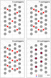 |
Fig. 1 BINGO beams on the sky and outriggers and four different outriggers pointing. In the case of ten outriggers, the pointings directly overlap with some of the BINGO beams in order to investigate how two equal outriggers pointing in the same direction at the same time affects the localization. The red × outriggers and the blue + outriggers are equal telescopes pointing in same directions. |
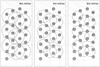 |
Fig. 2 BINGO horns and nine outrigger beams for three different mirror sizes. The dashed lines show the areas restricted by the FWHM defined in Eq. (3). |
3.1 Cosmological population
3.1.1 Redshift distribution
The spatial distribution of FRBs is not yet known due to the small number of measured redshifts of the associated host galaxies (Heintz et al. 2020). Some redshift distributions for FRBs have been considered over the years, including a Poisson distribution P(z) = ze−z, motivated by the distribution of gamma-ray bursts (Zhou et al. 2014; Yang & Zhang 2016), and a redshift distribution following the galaxy distribution P(z) = z2e−βz (Hagstotz et al. 2022). The alternative possibility used in this work is when the source of the FRBs is homogeneous in the co-moving volume. The source may not be perfectly homogeneous (Binggeli et al. 1988; Luo et al. 2018), but due to the still limited number of localized FRBs, a spatial distribution uniform in co-moving volume can serve as a first-order approximation of fz(z) (Luo et al. 2018; Chawla et al. 2022):
 (17)
(17)
where ∂V/(∂ω∂z) is the differential co-moving volume per unit solid angle per unit redshift, c is the speed of light, r(z) is the co-moving distance, and  is the parameterized version of the first Friedmann–Lemaitre equation. We used the best-fit values from the Planck Collaboration (Planck Collaboration VI 2020) for the matter density parameter, ωm = 0.31; dark energy density parameter, ωλ = 0.69; and Hubble constant today, H0 = 67.4 km s−1 Mpc−1. The term (1 + z) takes into account the time dilation due to cosmic expansion. The redshift is sampled according to the distribution in Eq. (17) for up to the maximum value of zmax = 10.
3.1.2 Luminosity distribution
The luminosity function of FRBs is also still not well understood, and although log-normal or power-law distributions have previously been used (Caleb et al. 2016), the Schechter function (Schechter 1976) adopted in Luo et al. (2018, 2020) seems to be favored over others (Petroff et al. 2019). Thus, we assume here that it is given by
 (18)
(18)
where L★ is the upper cutoff luminosity, φ★ is a normalization constant, and γ is the power-law index. These parameters were constrained in Luo et al. (2020) using 46 FRBs: L* = 2.9 × 1044 erg s−1, φ* = 339 Gpc−3 yr−1 and γ = −1.79.
3.1.3 Spectral index
The flux density of FRBs depends on the frequency as Sv ∝ vα, where the spectral index α can be positive or negative. In Luo et al. (2020), α = 0 was chosen due to being inspired by the apparently flat spectrum of FRB 121102 with 1 GHz of bandwidth (Gajjar et al. 2018). Chawla et al. (2017) reported a lack of FRB observations in the Green Bank Northern Celestial Cap survey at 350 MHz, indicating either a flat spectrum or a spectral turnover at frequencies above 400 MHz. However, some works (e.g., Lorimer et al. 2013) have assumed a spectral index similar to the one observed in pulsars (α = −1.4; Bates et al. 2013). Such a value is very close to the result obtained by Macquart et al. (2019) using 23 FRBs (α = −1.5). Based on these previous works, we chose to use two different values for the spectral index: α = 0 and α = −1.5. Similar values are also used in <mono>frbpoppy</mono> in its different population setups (Gardenier et al. 2019).
3.1.4 Number of sources
Several estimates of the all-sky rate of observable FRBs have been made. For instance, Thornton et al. (2013) estimated a rate of 104 sky−1 day−1 above a fluence of 3 Jy ms, while CHIME recently inferred a sky rate of 820 sky−1 day−1 above a fluence of 5 Jy ms at 600 MHz (CHIME/FRB Collaboration 2021). Luo et al. (2020) found event rate densities of 3.5 × 10⁴ Gpc−3 yr−1 above a luminosity of 1042 erg s−1, 5.0 × 10³ Gpc−3 yr−1 above 1043 erg s−1 and 3.7 × 10² Gpc−3 yr−1 above 1044 erg s−1. We estimated the rate per day per sky of detectable FRBs using the following expression (Luo et al. 2020)
 (19)
(19)
where fz(z) and ϕ(L) are given by Eqs. (17) and (18), respectively, and L0 is the intrinsic lower cutoff of the luminosity function inferred to be ≤9.1 × 1041 erg s−1. Using Eq. (19) with the values of the minimum flux density and observed pulse width for BINGO described in the next section, we estimated the total number of cosmic FRBs generated by FRBlip to be ~7 × 10⁴ per day of observation. In the next sections, we describe the methodology used to estimate the detection rate for BINGO, which will be a fraction of this cosmic population.
3.2 Sensitivity maps
The simplest way to estimate the detection rate is to follow the approach adopted by Luo et al. (2020), also used in Abdalla et al. (2022a), through the equation4
 (20)
(20)
The difference between Eqs. (19) and (20) is that the former assumes an all-sky rate, while the latter is calculated for the BINGO field of view and for redshift values bounded by the frequency range.
The minimum luminosity Lmin in the lower limit of integration is the maximum function max[L0, Lthre], where Lthre depends on the spectral index α and the antenna pattern
 (21)
(21)
where ∆v = v2 − v1, Smin is the telescope minimum flux density defined in Eq. (5)), and (S /N)thre indicates the minimum allowed value for the S/N, ensuring that we are counting only the objects rendering a minimum S/N luminosity value. The detection rate per unit of time was found by integrating over the telescope field of view,
 (22)
(22)
where this angular integration is performed using <mono>HEALPix</mono> (Górski et al. 2005) through <mono>astropy-healpix</mono> (Astropy Collaboration 2018)
 (23)
(23)
where npix and ωpix depend on the resolution (nside) of the <mono>HEALPix</mono> map. Detection rate estimates for the BINGO configurations described previously are shown in Fig. 6. The limitation of the present approach lies in the fact that computing complex quantities as the observation rates over the baselines is very costly. Indeed, to compute the detection rate of at least two baselines, we have to compute the sensitivity map for all the possible pairs of baselines. For three baselines, we must compute the detection rate for all possible combinations of three baselines, and so on.
3.3 FRBlip
To compute all the quantities described in the previous sections, we developed <mono>FRBlip</mono>5, a new <mono>Python</mono> package that generates mock catalogs, sorting the physical quantities as random numbers through the distributions described in Sect. 3.1. The information about the cosmic population is coded inside an object called <mono>FastRadioBursts</mono>, and the telescopes in objects of the type <mono>RadioTelescope</mono>. The results of observations come from the interaction between these two entities. To sort random numbers in the described distributions, the code uses the rv_continuous generic class from the <mono>scipy.stats</mono> module to construct, by subclassing, new classes that implement each distribution. This is a high-level tool that allows the developer to implement a random number generator of any distribution. Another important tool is the <mono>astropy.coordinates</mono> module, which is used to transform the non-local spherical coordinates to local coordinates at the telescope site in order to perform the observations.
The dependencies of the <mono>FRBlip</mono> include traditional <mono>Python</mono> numerical libraries, such as <mono>Numpy</mono> (Harris et al. 2020), <mono>Scipy</mono> (Virtanen et al. 2020), and <mono>Pandas</mono> (pandas development team 2020); high performance collection libraries, such as <mono>Xarray</mono> (Hoyer & Hamman 2017) and <mono>Sparse</mono>; the physical numerical libraries <mono>astropy</mono> (Astropy Collaboration 2018), <mono>HEALpix</mono> (Górski et al. 2005), and <mono>Pygedm</mono> (Price et al. 2021); and the numerical computing packages for cosmology, <mono>CAMB</mono> (Lewis & Bridle 2002) and <mono>PyCCL</mono> (Chisari et al. 2019).
4 Results and discussion
4.1 Detecting bursts
We discuss our evaluation of a more accurate detection rate in this section. We generated cosmological FRB mock catalogs using <mono>FRBlip</mono> and counted how many of those would be detected by BINGO, its outriggers, and the total BIS in different scenarios. In order to validate these results, we compare them with the sensitivity map results (which we label as “exact”). The key quantity is the yearly rate.
In order to reduce the computational processing, we performed a resampling over the mock of an one-day event. The idea behind the approach is that the most costly computational process is the coordinate transformation. Thus, avoiding this step reduces the processing time. To do so, we sampled by first generating one day of cosmological FRBs. Then we resampled over all the variables but the sky positions (right ascension and declination) to generate one more day. We created a mock of one year of events by taking this step further 363 times.
This procedure was then repeated 1000 times until we had enough data to adequately fit a Poisson distribution, which we did by using the <mono>statsmodels</mono> library (Seabold & Perktold 2010).
We first present the detectability of individual telescopes. In Fig. 3, we show the redshift distribution of the FRBs seen by only the main BINGO telescope(that is, without the outriggers; with S /N ≥ 1) over five years (purple histogram) compared with all the FRBs in the sky in one day (gray histogram in Fig. 3). We also compared this histogram in the figure with the exact distribution (purple continuous curve) computed from the sensitivity maps (Eq. (23)). We observed that the histogram is well bounded inside the 95% confidence level (C.L.; represented by the purple-shaded region). The red dashed line in the figure is the power log-normal6 distribution fitted on the complete 1000 years of simulation, and it is in good agreement with the exact value with a 95% C.L.
The number of FRBs increases with the redshift since the volume also increases until it reaches a maximum value. After that, it starts decreasing because the luminosity limit begins to dominate. The number of FRBs reaches a maximum value at z ≃ 1.8, where the rate becomes smaller than one. Therefore, we can interpret  , that is, the maximum effective redshift or the depth of the survey.
Figure 4 shows how the detection rate of FRBs varies with the S/N for the different telescope configurations described in Sect. 2. In all cases, we observed that the  values inferred from the power log-normal distribution, fitted from the mocks, are in agreement with the exact value with a 95% C.L. This alternative method to infer
  is important to determine the depth of the survey since we cannot compute the exact values from sensitivity maps, as discussed in Sect. 3.2.
In Fig. 5, we show the luminosity (left) and density flux (right) distributions. Fainter objects are more difficult to observe, as expected because it is more probable to have a density flux smaller than the minimum  . In order to illustrate the fraction of the distributions observed by BINGO, we compare the histograms of the cosmic distributions in one day with the ones observed by BINGO in 5 yr.
Finally, we show in Fig. 6 the detection rates obtained from mocks and the rates computed with the sensitivity maps, evidencing the agreement between the methods. The rates from individual outriggers (top panel in the figure) are less than one per year; however, the interferometry system, which integrates nine of the telescopes, can increase the BINGO detection rate by about 20%. For the case of interferometry, we have not computed the exact distributions, due to the reasons discussed at the end of Sect. 3.2. Thus, we needed an alternative method to infer the depth of these interferometric cases.
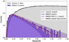 |
Fig. 3 Redshift distribution of the FRBs with S /N ≥ 1 observed by BINGO in 5 years (purple histogram) compared with all the cosmic bursts in 1 day (grey histogram). The exact cosmic distribution is shown with the black dashed line, the exact distribution for BINGO is represented by the solid purple distribution, and the shaded region is the exact 95% C.L. from the Poisson distribution. The red dashed line is the power log-normal distribution fitted from the 1000-year mock observation. |
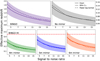 |
Fig. 4 Maximum effective redshift for different BINGO configurations varying from S/N ≥ 5 to S/N ≥ 15. When comparing the exact solution from sensitivity maps (solid lines) with the fitted power log-normal distribution (dashed lines), we note that they are in agreement with the exact solution in 95% C.L. (shaded regions). The red dashed line shows the maximum redshift of the BINGO HI survey. |
4.2 Localizing bursts
In this section, we evaluate the effectiveness of BIS to localize FRBs. We assumed a perfect delay compensation, that is, the exact time delay between the telescopes that compose each baseline is known. In this case, the S/N detection of localizing an FRB increases with the number of baselines that are used to observe it. Therefore, we had to select the better BIS configuration between the two options: more outriggers with narrower beam widths or fewer outriggers with wider beam widths. Unless otherwise stated, we use a flat spectrum in this section.
The number of FRBs detected by different baselines depends on the number of outriggers used in the system and the size of the mirror. The relevant instrumental parameters for FRB detection are sensitivity and field of view. The field of view generally varies inversely with the mirror size, while sensitivity increases with increasing mirror size. Ultimately, the choice of mirror size depends on the number of outriggers built and on the number of baselines needed to detect the same FRB. Increasing the number of outriggers also increases the collecting area and in turn reduces the minimum flux density.
To decide the best configuration for a BIS composed only of single horn outriggers, we had to define the following points: (i) the number of baselines an FRB must be observed by to have its position well inferred; (ii) the number of outriggers that we can construct; and (iii) the kind of outriggers that will be constructed. The answer to the first point depends only on how effective the pipeline to infer the positions is. Assuming that a minimum of two baselines is enough to pinpoint the source position from Fig. 7, we may infer the best type of outrigger for each configuration.
With five outriggers, the best choice is the 4-m mirror. For seven outriggers, the performance of the 4-m and 5-m mirrors are almost the same. For nine outriggers, the 4-m, 5-m, and 6-m mirrors perform approximately equally, and with ten outriggers, the 6-m mirror is the best. If we make the localization more restrictive, requiring at least three baselines, the picture changes a bit. With five outriggers, for instance, the horn with no mirror performs best, while for the other configurations (seven, nine, and ten outriggers), the 4-m mirror produces the best result.
The number of outriggers also depends on the number of baselines needed to permit a good localization of the source. In order to understand how the number of detections per baseline affects our results, we show in Fig. 7 the fraction of detected FRBs as a function of the number of baselines that detected a given FRB. We set the S/N to ten or higher. For this illustrative choice of S/N, we observed that the fraction of detected FRBs follows the same behavior in all four different panels of Fig. 7. The outriggers with a 4-m size detect more (or at least the same number) events than the ones with larger mirrors, with the exception of ten outriggers with two baselines. However, if more baselines detect the same FRB, then the naked horn is the best option with five or seven outriggers, that is, with five outriggers, the naked horn is better if the detections are made by three baselines or more, and with seven outriggers, the naked horn is better if the detections are made by four baselines or more, and so forth.
So far we have estimated the detection rates considering that the baselines and the autocorrelations have the same S/N threshold. However, this choice is arbitrary, and we may set a different approach, for instance, to first select a group of candidates observed by the main BINGO telescope and then filter this group with a different choice of S/N to define a detection in a baseline. In order to investigate how these different choices would affect our results, we defined a set of values for the S/N that would categorize an FRB as a candidate, a detection, an interferometry detection (for the cross-correlation between the main BINGO telescope and its outriggers), and localizations in one, two, or three baselines. This set of definitions is shown in Table 3.
In Table 3, the condition s1, corresponding to the label “Candidates” and S/N ≥ 1, was chosen to select the events that might be an actual FRB detection. Such an S/N does not need to be much larger than one and can occur either in auto- or cross-correlation since at this level we are simply looking for at least one baseline that received a potential signal. For the label “Detection” (meaning an actual detection), we chose s2 = 5 in order to pick candidates that certainly would be detected by the telescope. The same occurs for s3 in the interferometric detection, although in this step we already know that a detection occurred. In this case, we selected s3 = 3 because we are interested in knowing if the FRBs would be clearly detected in the interferometry side, with the goal being to pinpoint the source location. Furthermore, we needed to avoid the situation where the interferometric detection has an S/N larger than s3 , but no individual baseline has S/N > 1. We needed to guarantee that at least the number of baselines we are interested in (one, two, or three) are measuring the signal with a consistent S/N value, and for this we selected s4 = 2.
In Table 4 and in the top panel of Fig. 8, we show the results for the categorization described in Table 3. In Fig. 9, we show the distribution of events in the focal plane for two different outrigger setups.
The number of candidates increases slightly with the increase in the number of outriggers and mirror sizes. On the other hand, the number of detections, interferometric detections, and localizations using one baseline increase considerably with the number of outriggers and mirror sizes. The localizations using two or three baselines, however, are almost in all cases larger for a configuration of a 4-m mirror with five, seven, or nine outriggers. The number of localizations for a specific mirror size roughly increases with the number of outriggers. However, this does not always mean an increase in coverage area, and the exception is the scenario with ten outriggers, where there are many overlaps between the outriggers’ beams and that of the main BINGO (as can be seen from Fig. 1). Thus, in practice, the total observed area is less than the area of the scenario with five outriggers. As can be seen in Table 5 and in bottom panel of Fig. 8, the effective maximum redshift is between two and three for candidates and detections, but it is generally reduced to 0.5–1 for the localization.
We concluded from this analysis that narrow beams (i.e., horns with bigger mirrors) can observe higher redshift values but that an FRB can be observed by more beams with a set composed of larger beams. This problem can be compensated for by introducing more telescopes into the BIS, which expands the observed area.
As can be seen in Table 4, the introduction of more outriggers can multiply the detection rates by several factors. Regarding the localizations, the performance saturates for one, two, or three baselines and reach hundreds of localized bursts. We observed a similar behavior in Table 5 for the redshift, where the outriggers improve the depth of the survey. The results are virtually the same with one, two, or three baselines, exceeding the value of  and reaching 1.28 in the best case.
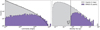 |
Fig. 5 Luminosity and flux density distributions. Left: number of events as a function of the luminosity distribution. Right: number of events but as a function of the flux density distribution. The estimates are for cosmic FRBs during 1 day (gray) and observed FRBs, with S/N ≥ 1, during the 5 years of the BINGO Phase 1 mission (purple). |
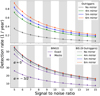 |
Fig. 6 Detection rate estimates for BINGO. Top: mean detection rate for individual outriggers with the configuration as described in Sect. 2 and Table 2. Bottom: detection rate for the complete BIS (main BINGO and outriggers). In both cases, we show the detection rates computed by the two methods: sensitivity maps (solid lines) and mock catalogs created with <mono>FRBlip</mono> (scatter). |
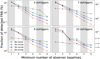 |
Fig. 7 Fraction of observed bursts (S/N ≥ 10) as a function of baselines that detected the same events for the sixteen different BIS configurations. |
Different conditions and S/N thresholds.
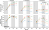 |
Fig. 8 Yearly detection rate (top) and effective maximum redshift (bottom) for prescription described in Table 3 as a function of the mirror size for five, seven, nine, and ten outriggers. |
5 Conclusions and perspectives
In this work, we investigated the capabilities of the BINGO telescope to search for and detect FRBs as well as how a set of outriggers can be used to localize the events in the sky through the BIS. We considered a single, naked horn plus three different mirror sizes for the outriggers, all with single horns, for five, seven, nine, and ten outriggers. In order to produce synthetic FRBs and calculate the detection rates, we developed the code <mono>FRBlip</mono>.
Using different methodologies to define detection and localization through baselines, we estimated that BINGO alone would be able to observe dozens of FRBs per year, around 50 with S / N ≥ 5 and 20 with S / N ≥ 15 (for α = 0, as used in Eq. (21)), in agreement with what was previously calculated (Abdalla et al. 2022a). The introduction of outriggers can improve the total detection rate by about 20% with nine outriggers.
Regarding the localization, if we use two baselines, then the best scenario is when outriggers have a 4-m mirror, and the estimates improve from 10.3 events per year (for five outriggers) to 15.9 events per year (for seven outriggers), 18.4 events per year (for nine outriggers), and 20.1 events per year (for ten outriggers), as shown in Table 4. However, if the localization is through three baselines, the best case is to have seven, nine, or ten outriggers with a 4-m mirror, yielding 10 to 12.5 events per year. With five outriggers, the best option would be outriggers without mirrors, which would reach seven events per year.
BINGO has the potential to increase the number of localized FRBs such that it will be possible to better identify the host galaxy and therefore investigate inherent aspects of galaxy science related to FRB distributions. These aspects may include which types of galaxies allow FRB production and a possible relationship between FRB distribution and galaxy morphology and formation. Additionally, FRB detection and localization would contribute to the exploration of redshift space, which in turn can be used to better constrain cosmological parameters (Walters et al. 2018). Finally, an increased number of identified sources can help elucidate the distribution functions of FRBs, such as the redshift distribution used in this work.
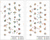 |
Fig. 9 Distribution of candidates and detections for two outrigger configurations. |

Acknowledgements
The BINGO project is supported by São Paulo Research Foundation (FAPESP) grant 2014/07885-0. R.G.L. thanks Rui Luo and Mike Peel for their useful comments. J.Z acknowledges support from the Ministry of Science and Technology of China (grant Nos. 2020SKA0110102). L.S. is supported by the National Key R&D Program of China (2020YFC2201600) and NSFC grant 12150610459. L.B., A.R.Q., and M.V.S. acknowledge PRONEX/CNPq/FAPESQ-PB (Grant no. 165/2018). A.R.Q. acknowledges FAPESQ-PB support and CNPq support under process number 310533/2022-8. C.A.W. acknowledges CNPq for the research grants 407446/2021-4 and 312505/2022-1. C.P.N. thanks Serrapilheira and São Paulo Research Foundation (FAPESP; grant 2019/06040-0) for financial support Y. S. is supported by grant from NSFC (Grant No. 12005184). X. Z. is supported by grant from NSFC (Grant No. 12005183). P.M.: This study was financed in part by the Coordenação de Aperfeiçoamento de Pessoal de Nível Superior – Brasil (CAPES) – Finance Code 001. This study was financed in part by the São Paulo Research Foundation (FAPESP) through grant 2021/08846-2 and 2023/07728-1. J.R.L.S. thanks CNPq (Grant nos. 420479/2018-0, and 309494/2021-4), and PRONEX/CNPq/FAPESQ-PB (Grant nos. 165/2018, and 0015/2019) for financial support. This study was financed in part by the Coordenação de Aper- feiçoamento de Pessoal de Nível Superior – Brazil (CAPES) – Finance Code 88887.622333/2021-00. The BINGO project thanks FAPESQ and the government of the State of Paraiba for funding the project. This research made use of <mono>astropy</mono> (Astropy Collaboration 2018), <mono>healpy</mono> (Zonca et al. 2019), <mono>numpy</mono> (Harris et al. 2020), <mono>scipy</mono> (Virtanen et al. 2020) and <mono>matplotlib</mono> (Hunter 2007). The authors thank the anonymous referee for the very useful report.
Appendix A Relation between bolometric luminosity and luminosity in Luo et al. (2020)
The energy released per unit of frequency interval in the rest-frame, Ev′, is given by (Lorimer et al. 2013)
 (A.1)
(A.1)
Here, k is a constant, α is the spectral index, and v′ is the rest-frame frequency.
The bolometric luminosity is then obtained by integrating the energy over all possible emitted frequencies
 (A.2)
(A.2)
Here, we have omitted the top-hat pulse of width present in Lorimer et al. (2013) and v′ = (1 + ɀ)v.
The luminosity in Luo et al. (2020), however, is a sub-part of the bolometric luminosity since the assumed spectral width is vLuo, high − vLuo, low = 1 GHz. We can then write the “Luo” luminosity as
 (A.3)
(A.3)
where Bv′ is a rectangular function defined as Bv′ = 1 for  , and Bv′ = 0 otherwise. We note that LLuo = Lbol if
  and
and  .
.
Using Equations (A.2) and (A.3), we obtain the relation between the two luminosities
 (A.4)
(A.4)
Therefore, using the above relation in Eq. (10), we obtain Eq. (13). The luminosities used in Section 3 are the Luo luminosities LLuo, but we have removed the subscript “Luo.”
References
- Abdalla, E., & Marins, A. 2020, Int. J. Mod. Phys. D, 29, 2030014 [NASA ADS] [CrossRef] [Google Scholar]
- Abdalla, E., Ferreira, E. G. M., Landim, R. G., et al. 2022a, A&A, 664, A14 [NASA ADS] [CrossRef] [EDP Sciences] [Google Scholar]
- Abdalla, F. B., Marins, A., Motta, P., et al. 2022b, A&A, 664, A16 [NASA ADS] [CrossRef] [EDP Sciences] [Google Scholar]
- Astropy Collaboration (Price-Whelan, A. M., et al.) 2018, AJ, 156, 123 [Google Scholar]
- Bannister, K. W., Shannon, R. M., Macquart, J. P., et al. 2017, ApJ, 841, L12 [NASA ADS] [CrossRef] [Google Scholar]
- Bates, S. D., Lorimer, D. R., & Verbiest, J. P. W. 2013, MNRAS, 431, 1352 [Google Scholar]
- Battye, R. A., Browne, I. W. A., Dickinson, C., et al. 2013, MNRAS, 434, 1239 [NASA ADS] [CrossRef] [Google Scholar]
- Bertolami, O., & Landim, R. G. 2018, Phys. Dark Univ., 21, 16 [NASA ADS] [CrossRef] [Google Scholar]
- Bhandari, S., Heintz, K. E., Aggarwal, K., et al. 2022, AJ, 163, 69 [NASA ADS] [CrossRef] [Google Scholar]
- Binggeli, B., Sandage, A., & Tammann, G. A. 1988, ARA&A, 26, 509 [NASA ADS] [CrossRef] [Google Scholar]
- Caleb, M., Flynn, C., Bailes, M., et al. 2016, MNRAS, 458, 708 [Google Scholar]
- Caleb, M., Flynn, C., Bailes, M., et al. 2017, MNRAS, 468, 3746 [NASA ADS] [CrossRef] [Google Scholar]
- Chawla, P., Kaspi, V. M., Josephy, A., et al. 2017, ApJ, 844, 140 [NASA ADS] [CrossRef] [Google Scholar]
- Chawla, P., Kaspi, V. M., Ransom, S. M., et al. 2022, ApJ, 927, 35 [NASA ADS] [CrossRef] [Google Scholar]
- CHIME/FRB Collaboration (Amiri, M., et al.) 2018, ApJ, 863, 48 [NASA ADS] [CrossRef] [Google Scholar]
- CHIME/FRB Collaboration (Andersen, B. C., et al.) 2020, Nature, 587, 54 [Google Scholar]
- CHIME/FRB Collaboration (Amiri, M., et al.) 2021, ApJS, 257, 59 [NASA ADS] [CrossRef] [Google Scholar]
- Chisari, N. E., Alonso, D., Krause, E., et al. 2019, ApJS, 242, 2 [Google Scholar]
- Connor, L., van Leeuwen, J., Oostrum, L. C., et al. 2020, MNRAS, 499, 4716 [CrossRef] [Google Scholar]
- Cordes, J. M., & Lazio, T. J. W. 2002, ArXiv e-prints [arXiv: 0207156] [Google Scholar]
- Costa, A. A., Landim, R. G., Novaes, C. P., et al. 2022, A&A, 664, A20 [NASA ADS] [CrossRef] [EDP Sciences] [Google Scholar]
- de Mericia, E. J., Santos, L. C. O., Wuensche, C. A., et al. 2023, A&A, 671, A58 [NASA ADS] [CrossRef] [EDP Sciences] [Google Scholar]
- Fornazier, K. S. F., Abdalla, F. B., Remazeilles, M., et al. 2022, A&A, 664, A18 [NASA ADS] [CrossRef] [EDP Sciences] [Google Scholar]
- Gajjar, V., Siemion, A. P. V., Price, D. C., et al. 2018, ApJ, 863, 2 [NASA ADS] [CrossRef] [Google Scholar]
- Gardenier, D. W., van Leeuwen, J., Connor, L., & Petroff, E. 2019, A&A, 632, A125 [NASA ADS] [CrossRef] [EDP Sciences] [Google Scholar]
- Górski, K. M., Hivon, E., Banday, A. J., et al. 2005, ApJ, 622, 759 [Google Scholar]
- Hagstotz, S., Reischke, R., & Lilow, R. 2022, MNRAS, 511, 662 [CrossRef] [Google Scholar]
- Harris, C. R., Millman, K. J., van der Walt, S. J., et al. 2020, Nature, 585, 357 [NASA ADS] [CrossRef] [Google Scholar]
- Heintz, K. E., Prochaska, J. X., Simha, S., et al. 2020, ApJ, 903, 152 [NASA ADS] [CrossRef] [Google Scholar]
- Hoyer, S., & Hamman, J. 2017, J. Open Res. Softw., 5, 10 [CrossRef] [Google Scholar]
- Hunter, J. D. 2007, Comput. Sci. Eng., 9, 90 [NASA ADS] [CrossRef] [Google Scholar]
- Kraus, J. D., Tiuri, M., Räisänen, A. V., & Carr, T. D. 1986, Radio Astronomy, 69 (Ohio: Cygnus-Quasar Books Powell) [Google Scholar]
- Landim, R. G. 2020, Eur. Phys. J. C, 80, 913 [NASA ADS] [CrossRef] [Google Scholar]
- Lewis, A., & Bridle, S. 2002, Phys. Rev. D, 66, 103511 [Google Scholar]
- Liccardo, V., de Mericia, E. J., Wuensche, C. A., et al. 2022, A&A, 664, A17 [NASA ADS] [CrossRef] [EDP Sciences] [Google Scholar]
- Linder, E. V. 2020, Phys. Rev. D, 101, 103019 [NASA ADS] [CrossRef] [Google Scholar]
- Liu, B., Li, Z., Gao, H., & Zhu, Z.-H. 2019, Phys. Rev. D, 99, 123517 [CrossRef] [Google Scholar]
- Lorimer, D. R., Bailes, M., McLaughlin, M. A., Narkevic, D. J., & Crawford, F. 2007, Science, 318, 777 [Google Scholar]
- Lorimer, D., Karastergiou, A., McLaughlin, M., & Johnston, S. 2013, MNRAS, 436, 5 [Google Scholar]
- Luo, R., Lee, K., Lorimer, D. R., & Zhang, B. 2018, MNRAS, 481, 2320 [Google Scholar]
- Luo, R., Men, Y., Lee, K., et al. 2020, MNRAS, 494, 665 [NASA ADS] [CrossRef] [Google Scholar]
- Macquart, J. P., Shannon, R. M., Bannister, K. W., et al. 2019, ApJ, 872, L19 [NASA ADS] [CrossRef] [Google Scholar]
- Marins, A., Abdalla, F. B., Fornazier, K. S. F., et al. 2022, ArXiv e-prints [arXiv:2209.11701] [Google Scholar]
- Masui, K., Lin, H.-H., Sievers, J., et al. 2015, Nature, 528, 523 [NASA ADS] [CrossRef] [Google Scholar]
- Muñoz, J. B., & Loeb, A. 2018, Phys. Rev. D, 98, 103518 [CrossRef] [Google Scholar]
- Muñoz, J. B., Kovetz, E. D., Dai, L., & Kamionkowski, M. 2016, Phys. Rev. Lett., 117, 091301 [CrossRef] [Google Scholar]
- Novaes, C. P., Zhang, J., de Mericia, E. J., et al. 2022, A&A, 666, A83 [NASA ADS] [CrossRef] [EDP Sciences] [Google Scholar]
- Ocker, S. K., Cordes, J. M., Chatterjee, S., & Gorsuch, M. R. 2022, ApJ, 934, 71 [NASA ADS] [CrossRef] [Google Scholar]
- pandas development team 2020, https://doi.org/10.5281/zenodo.3509134 [Google Scholar]
- Astor-Marazuela, I., Connor, L., van Leeuwen, J., et al. 2021, Nature, 596, 505 [NASA ADS] [CrossRef] [Google Scholar]
- Petroff, E., Hessels, J. W. T., & Lorimer, D. R. 2019, A&ARv, 27, 4 [NASA ADS] [CrossRef] [Google Scholar]
- Petroff, E., Hessels, J. W. T., & Lorimer, D. R. 2022, A&ARv, 30, 2 [NASA ADS] [CrossRef] [Google Scholar]
- Planck Collaboration VI. 2020, A&A, 641, A6 [NASA ADS] [CrossRef] [EDP Sciences] [Google Scholar]
- Platts, E., Weltman, A., Walters, A., et al. 2019, Phys. Rept., 821, 1 [CrossRef] [Google Scholar]
- Pleunis, Z., Michilli, D., Bassa, C. G., et al. 2021, ApJ, 911, L3 [NASA ADS] [CrossRef] [Google Scholar]
- Price, D. C., Flynn, C., & Deller, A. 2021, PASA, 38, e038 [NASA ADS] [CrossRef] [Google Scholar]
- Qiang, D.-C., & Wei, H. 2020, JCAP, 04, 023 [CrossRef] [Google Scholar]
- Sammons, M. W., Macquart, J.-P., Ekers, R. D., et al. 2020, ApJ, 900, 122 [NASA ADS] [CrossRef] [Google Scholar]
- Schechter, P. 1976, ApJ, 203, 297 [Google Scholar]
- Seabold, S., & Perktold, J. 2010, in Proceedings of the 9th Python in ScienceConference, eds. S. van der Walt, & J. Millman, 92 [CrossRef] [Google Scholar]
- Shao, L., & Zhang, B. 2017, Phys. Rev. D, 95, 123010 [NASA ADS] [CrossRef] [Google Scholar]
- Spitler, L. G., Cordes, J. M., Hessels, J. W. T., et al. 2014, ApJ, 790, 101 [NASA ADS] [CrossRef] [Google Scholar]
- Tendulkar, S. P., Bassa, C., Cordes, J. M., et al. 2017, ApJ, 834, L7 [NASA ADS] [CrossRef] [Google Scholar]
- Thompson, A. R., Moran, J. M., & Swenson, G. W. 2017, Interferometry andSynthesis in Radio Astronomy (Springer Nature) [CrossRef] [Google Scholar]
- Thornton, D., Stappers, B., Bailes, M., et al. 2013, Science, 341, 53 [NASA ADS] [CrossRef] [Google Scholar]
- Tingay, S. J., & Kaplan, D. L. 2016, ApJ, 820, L31 [NASA ADS] [CrossRef] [Google Scholar]
- Tingay, S. J., Trott, C. M., Wayth, R. B., et al. 2015, AJ, 150, 199 [NASA ADS] [CrossRef] [Google Scholar]
- Virtanen, P., Gommers, R., Oliphant, T. E., et al. 2020, Nat. Meth., 17, 261 [Google Scholar]
- Walker, R. 1989, “Sensitivity” in Very Long Baseline Interferometry, eds. M. Felli & R.E. Spencer (Kluwer: Dordrecht), 163 [CrossRef] [Google Scholar]
- Walters, A., Weltman, A., Gaensler, B., Ma, Y.-Z., & Witzemann, A. 2018, ApJ, 856, 65 [NASA ADS] [CrossRef] [Google Scholar]
- Walters, A., Ma, Y.-Z., Sievers, J., & Weltman, A. 2019, Phys. Rev. D, 100, 103519 [NASA ADS] [CrossRef] [Google Scholar]
- Wang, Y. K., & Wang, F. Y. 2018, A&A, 614, A50 [NASA ADS] [CrossRef] [EDP Sciences] [Google Scholar]
- Wei, J.-J., Gao, H., Wu, X.-F., & Mészáros, P. 2015, Phys. Rev. Lett., 115, 261101 [NASA ADS] [CrossRef] [Google Scholar]
- Wu, Q., Yu, H., & Wang, F. Y. 2020, ApJ, 895, 33 [NASA ADS] [CrossRef] [Google Scholar]
- Wuensche, C. A., Villela, T., Abdalla, E., et al. 2022, A&A, 664, A15 [NASA ADS] [CrossRef] [EDP Sciences] [Google Scholar]
- Xing, N., Gao, H., Wei, J., et al. 2019, ApJ, 882, L13 [NASA ADS] [CrossRef] [Google Scholar]
- Yang, Y.-P., & Zhang, B. 2016, ApJ, 830, L31 [Google Scholar]
- Yao, J., Manchester, R. N., & Wang, N. 2019, Astrophysics Source Code Library [record ascl:1908.022] [Google Scholar]
- Yu, H., & Wang, F. Y. 2017, A&A, 606, A3 [NASA ADS] [CrossRef] [EDP Sciences] [Google Scholar]
- Yu, H., & Wang, F. 2018, Eur. Phys. J. C, 78, 692 [NASA ADS] [CrossRef] [Google Scholar]
- Yu, H., Xi, S., & Wang, F. 2018, ApJ, 860, 173 [NASA ADS] [CrossRef] [Google Scholar]
- Zhang, J., Motta, P., Novaes, C. P., et al. 2022, A&A, 664, A19 [NASA ADS] [CrossRef] [EDP Sciences] [Google Scholar]
- Zhao, Z.-W., Li, Z.-X., Qi, J.-Z., et al. 2020, ApJ, 903, 83 [NASA ADS] [CrossRef] [Google Scholar]
- Zhou, B., Li, X., Wang, T., Fan, Y.-Z., & Wei, D.-M. 2014, Phys. Rev. D, 89, 107303 [NASA ADS] [CrossRef] [Google Scholar]
- Zhu, W., & Feng, L.-L. 2021, ApJ, 906, 95 [NASA ADS] [CrossRef] [Google Scholar]
- Zonca, A., Singer, L., Lenz, D., et al. 2019, J. Open Source Softw., 4, 1298 [Google Scholar]
See https://www.wis-tns.org/ for the official list of events.
See https://frbtheorycat.org/ for a list of different models.
We have implicitly assumed that there are at least two nonparallel baselines. We have already identified places near the main telescope where the outriggers might be installed, between ~10 and 40 km in such a way that the angular precision is ~1–3 arcsec.
For simplicity, we did not assume the impact on the FRB pulse due to intrachannel smearing at high dispersion measures or scattering (Petroff et al. 2019; Ocker et al. 2022).
All Tables
All Figures
|
Fig. 1 BINGO beams on the sky and outriggers and four different outriggers pointing. In the case of ten outriggers, the pointings directly overlap with some of the BINGO beams in order to investigate how two equal outriggers pointing in the same direction at the same time affects the localization. The red × outriggers and the blue + outriggers are equal telescopes pointing in same directions. |
| In the text | |
|
Fig. 2 BINGO horns and nine outrigger beams for three different mirror sizes. The dashed lines show the areas restricted by the FWHM defined in Eq. (3). |
| In the text | |
|
Fig. 3 Redshift distribution of the FRBs with S /N ≥ 1 observed by BINGO in 5 years (purple histogram) compared with all the cosmic bursts in 1 day (grey histogram). The exact cosmic distribution is shown with the black dashed line, the exact distribution for BINGO is represented by the solid purple distribution, and the shaded region is the exact 95% C.L. from the Poisson distribution. The red dashed line is the power log-normal distribution fitted from the 1000-year mock observation. |
| In the text | |
|
Fig. 4 Maximum effective redshift for different BINGO configurations varying from S/N ≥ 5 to S/N ≥ 15. When comparing the exact solution from sensitivity maps (solid lines) with the fitted power log-normal distribution (dashed lines), we note that they are in agreement with the exact solution in 95% C.L. (shaded regions). The red dashed line shows the maximum redshift of the BINGO HI survey. |
| In the text | |
|
Fig. 5 Luminosity and flux density distributions. Left: number of events as a function of the luminosity distribution. Right: number of events but as a function of the flux density distribution. The estimates are for cosmic FRBs during 1 day (gray) and observed FRBs, with S/N ≥ 1, during the 5 years of the BINGO Phase 1 mission (purple). |
| In the text | |
|
Fig. 6 Detection rate estimates for BINGO. Top: mean detection rate for individual outriggers with the configuration as described in Sect. 2 and Table 2. Bottom: detection rate for the complete BIS (main BINGO and outriggers). In both cases, we show the detection rates computed by the two methods: sensitivity maps (solid lines) and mock catalogs created with <mono>FRBlip</mono> (scatter). |
| In the text | |
|
Fig. 7 Fraction of observed bursts (S/N ≥ 10) as a function of baselines that detected the same events for the sixteen different BIS configurations. |
| In the text | |
|
Fig. 8 Yearly detection rate (top) and effective maximum redshift (bottom) for prescription described in Table 3 as a function of the mirror size for five, seven, nine, and ten outriggers. |
| In the text | |
|
Fig. 9 Distribution of candidates and detections for two outrigger configurations. |
| In the text | |
Current usage metrics show cumulative count of Article Views (full-text article views including HTML views, PDF and ePub downloads, according to the available data) and Abstracts Views on Vision4Press platform.
Data correspond to usage on the plateform after 2015. The current usage metrics is available 48-96 hours after online publication and is updated daily on week days.
Initial download of the metrics may take a while.