© ESO 2021

1. Introduction

The existence of fully convective low-mass stars has been predicted by theoretical stellar models at least since the 1950s (e.g., Limber 1958). Current stellar structure and evolution models indicate that stars with masses less than about 0.35 M_⊙ are fully convective (e.g., Chabrier & Baraffe 1997, 2000). However, until recently no direct observational evidence could be attached to this transition. A recent analysis of Gaia observations indicates a gap in the main sequence at spectral type M3, which is perhaps the most direct observational evidence of transition to full convection to date (Jao et al. 2018). The gap in the Hertzsprung–Russell diagram near the transition to full convection is presumed to be associated with an instability related to ³He burning in the core of the star, such that the core undergoes periods of radiative and convective phases before settling to a final either convectively stable or unstable state depending on the mass of the star (e.g., van Saders & Pinsonneault 2012; Baraffe & Chabrier 2018; Feiden et al. 2021). Furthermore, in the final stable configuration, stars just on the partially convective side of the transition have a substantial (roughly 40% of stellar radius) radiative core, implying a discontinuity in stellar structure around M = 0.35 M_⊙.

The transition to full convection is important from the point of view of stellar dynamo theory because of an ongoing debate regarding the origin of the solar large-scale magnetic field (e.g., Charbonneau 2020, and references therein). This debate revolves around the importance of the tachocline, a layer of strong shear just below the convection zone (CZ), and that of the CZ itself. In simplified terms, in the distributed dynamo scenario the magnetic fields are generated throughout the CZ and the tachocline is unimportant (e.g., Krause & Rädler 1980; Brandenburg 2005; Käpylä et al. 2006; Pipin & Kosovichev 2011), while in the flux-transport models (e.g., Dikpati & Charbonneau 1999; Hazra et al. 2014) the roles of these two scenarios are the opposite. In reality, however, stellar dynamos are likely to have ingredients from both scenarios.

The fact that there are no tachoclines in fully convective stars makes these objects highly interesting in view of dynamo theory. If M star magnetism showed a discontinuity at the transition to full convection, we might argue that the type of dynamo also changes across the transition. However, no conclusive observational evidence for such discontinuity has been detected so far (Donati et al. 2008; Morin et al. 2008, 2010; Kochukhov 2021), such that most activity indicators appear to be continuous across the transition to full convection (see however West et al. 2015; Mullan & Houdebine 2020). For example, the X-ray luminosity of fully convective M stars falls in line with partially convective stars (Wright & Drake 2016; Wright et al. 2018).

Observations of M stars shows a rich variety of possible magnetic states (see Kochukhov 2021, and references therein). Zeeman–Doppler imaging (ZDI) results of early-type (partially convective) M dwarfs tend to have relatively weak multipolar fields while stars around the transition to full convection often have strong dipole-dominated configurations (Donati et al. 2008). Intriguingly, rapidly rotating late-type M dwarfs can have either configuration, suggesting a possibility of bistable dynamo states (e.g., Gastine et al. 2013). The ZDI results of fully convective stars have not yet revealed any cyclicity, for example in terms of polarity reversals of the large-scale field. The lack of sufficiently long data series is a likely contributor to this. However, longer-term observations of other activity indicators, such as chromospheric emission, of a nearby slowly rotating (P_rot ≈ 90 days) fully convective star Proxima Centauri indicate an activity cycle of around seven years (Suárez Mascareño et al. 2016; Wargelin et al. 2017; Damasso et al. 2020; Klein et al. 2021). Another recent study found evidence of an activity cycle of roughly five years for the fully convective star Ross 128 with rotation period of more than 100 days (Ibañez Bustos et al. 2019, and references therein). Interestingly, an activity cycle of similar length has also been reported recently from a rapidly rotating fully convective star Gl 729 with P_rot ≈ 3 days (e.g., Ibañez Bustos et al. 2020).

Another aspect that makes low mass stars particularly interesting is that detecting Earth-sized planets on orbits suitable for life around M stars is much easier than for, for example solar mass stars. This is because M stars are less massive than the Sun, and as a result of their low luminosity the habitable planets must have close orbits, leading to a much larger radial velocity signal (e.g., Kasting et al. 2014). However, as noted above, M stars are very often magnetically active and that leads to effects such as starspots and Zeeman broadening, which can hinder radial velocity measurements. The magnetic activity of the host star is also of significance for the exoplanets such that they can be subject to violent flares and coronal mass ejections. Therefore, understanding convection and magnetic activity of M stars is of great importance in the search for possible life-supporting exoplanets.

Numerical simulations of fully convective stars are challenging because the CZ spans the entire radius of the star, implying strong density contrast and greatly varying spatial and temporal scales. Furthermore, the Mach numbers in the cores of fully convective stars are very low, thereby leading to a short acoustic timestep. A further complication arises owing to the singularity of commonly used spherical polar coordinates at the centre of the star. Most three-dimensional simulations of fully convective stars to date (e.g., Browning 2008; Browning et al. 2011; Gastine et al. 2013; Yadav et al. 2015a, 2016; Brown et al. 2020) have been made using anelastic equations, which bypass the acoustic timestep constraint. Furthermore, most of these simulations operate in spherical shells and the innermost core of the star is not modelled as a consequence of the coordinate singularity (see, however, Brown et al. 2020). Although it can be argued that the omission of a small core spanning at most a few per cent of stellar radius is likely to be insignificant for the global dynamics, additional boundary conditions need to be imposed around the central void. An exception is the study of Dobler et al. (2006) who used a star-in-a-box approach (see also Freytag et al. 2002; Dorch 2004; Woodward et al. 2019; Masada et al. 2020) in which a spherical star is embedded into a Cartesian cube. This approach allows the full star, including the centre, to be modelled. However, this comes at a cost of including the corners of the box that are unimportant for the interior dynamics of the star. This also implies that the spatial resolution of the star-in-a-box simulations is necessarily lower than in corresponding spherical shells models.

In the current study the star-in-a-box model of Dobler et al. (2006) is refined with developments from convection simulations in other contexts. This includes using heat conductivity based on Kramers opacity law (e.g., Brandenburg et al. 2000; Käpylä et al. 2017a) and a subgrid-scale (SGS) entropy diffusion that enables more realistic luminosities. Furthermore, one of the principal aims of the current study is to compare the results from the star-in-a-box models of fully convective stars with corresponding results obtained in spherical shells. Another point of interest is to compare the transitions of differential rotation and dynamo solutions as functions of rotation in fully convective stars. Numerical studies of partially convective stars indicate a transition from anti-solar (slow equator, fast poles) to solar-like (fast equator, slow poles) differential rotation (e.g., Gastine et al. 2014; Käpylä et al. 2014) around the rotation rate, where the advection and Coriolis forces are of the same order of magnitude, that is Coriolis (inverse Rossby) number unity. Furthermore, corresponding dynamo solutions progress from predominantly axisymmetric and quasi-steady solutions for slow rotation (e.g., Käpylä et al. 2017b; Strugarek et al. 2018), through oscillatory axisymmetric fields at intermediate rotation (e.g., Gilman 1983; Käpylä et al. 2012; Nelson et al. 2013), to non-axisymmetric azimuthal dynamo waves for rapid rotation (e.g., Cole et al. 2014; Yadav et al. 2015b; Viviani et al. 2018). A set of simulations with rotation periods in the range from 4.3 to 430 d are presented to study if, and where, such transitions in differential rotation and dynamos also occur in models of fully convective stars.

2. The model

The model is based on the star-in-a-box model presented in Dobler et al. (2006). A star of radius R is embedded into a Cartesian cube with a side half-length of H = 1.1R where all coordinates (x, y, z) run from −H to H. Motions and temperature fluctuations are damped for r >  R, where $r=\sqrt{x^2+y^2+z^2}$ is the spherical radius. The following set of equations of magnetohydrodynamics (MHD) are solved:

$$\begin{array}{cc}& \frac{\partial \mathit{A}}{\partial t}=\mathit{U}\times \mathit{B}-\eta {\mu }_0\mathit{J},\hfill \end{array}$$(1)

$$\begin{array}{cc}& \frac{\mathrm{D}ln\rho }{\mathrm{D}t}=-\mathbf{\nabla }·\mathit{U},\hfill \end{array}$$(2)

$$\begin{array}{cc}& \frac{\mathrm{D}\mathit{u}}{\mathrm{D}t}=-\mathbf{\nabla }\mathrm{\Phi }-\frac{1}{\rho }(\mathbf{\nabla }p-\mathbf{\nabla }·2\nu \rho \mathsf{S}+\mathit{J}\times \mathit{B})\hfill \\ \hfill & -2\mathbf{\Omega }\times \mathit{U}+{\mathit{f}}_{\mathrm{d}},\hfill \end{array}$$(3)

$$\begin{array}{cc}& T\frac{\mathrm{D}s}{\mathrm{D}t}=-\frac{1}{\rho }[\mathbf{\nabla }·({\mathit{F}}_{\mathrm{rad}}+{\mathit{F}}_{\mathrm{SGS}})+\mathcal{H}-\mathcal{C}]\hfill \\ \hfill & +2\nu {\mathsf{S}}^2+{\mu }_0\eta {\mathit{J}}^2,\hfill \end{array}$$(4)

where A is the magnetic vector potential, U is the velocity, B = ∇ × A is the magnetic field, J = ∇ × B/μ₀ is the current density, μ₀ is the permeability of vacuum, η is the magnetic diffusivity, D/Dt = ∂/∂t + U ⋅ ∇ is the advective derivative, ρ is the fluid density, Φ is the gravitational potential, p is the pressure, ν is the kinematic viscosity, S is the traceless rate-of-strain tensor with

$$\begin{array}{c}\hfill {\mathsf{S}}_{\mathit{ij}}=\frac{1}{2}(U_{i,j}+U_{j,i})-\frac{1}{3}{\delta }_{\mathit{ij}}\mathbf{\nabla }·\mathit{U},\end{array}$$(5)

where the commas denote differentiation, and δ_ij is the Kronecker delta. The expression Ω = (0, 0, Ω₀) is the rotation rate of the star, f_d is a damping function, T is the temperature, s is the specific entropy, F_rad is the radiative flux, F_SGS is the SGS entropy flux, and ℋ and 𝒞 describe heating and cooling, respectively.

The gas obeys an ideal gas equation of state with p = ℛρT, where ℛ = c_P − c_V is the universal gas constant, and c_P and c_V are the heat capacities at constant pressure and volume, respectively. The effects of degeneracy in the equation of state are neglected. The gravitational potential Φ is fixed in space and time and set up such that this quantity corresponds to an isentropic hydrostatic state of an M5 star (see Appendix A of Dobler et al. 2006) with

$$\begin{array}{c}\hfill \mathrm{\Phi }(r)=-\frac{\mathit{GM}}{R}\frac{a_0+a_2{r}^{\prime 2}+a_3{r}^{\prime 3}}{1+b_2{r}^{\prime 2}+b_3{r}^{\prime 3}+a_3{r}^{\prime 4}},\end{array}$$(6)

where G is the gravitational constant, M is the mass of the star, r′ = r/R and a₀ = 2.34, a₂ = 0.44, a₃ = 2.60, b₂ = 1.60, and b₃ = 0.21.

The term f_d describes damping of flows exterior to the star according to

$$\begin{array}{c}\hfill {\mathit{f}}_{\mathrm{d}}=-\frac{\mathit{U}}{{\tau }_{\mathrm{damp}}}{f}_{\mathrm{e}}(r),\end{array}$$(7)

where τ_damp is a damping timescale, and where f_e(r) is given by

$$\begin{array}{c}\hfill f_{\mathrm{e}}(r)=\frac{1}{2}(1+tanh\frac{r-r_{\mathrm{damp}}}{w_{\mathrm{damp}}}),\end{array}$$(8)

where r_damp  =  1.03R and w_damp  =  0.03R. The damping timescale, τ_damp ≈ 1 d, is short in comparison to all other relevant timescales in the system.

Radiation is taken into account through the diffusion approximation. The radiative flux is given by

$$\begin{array}{c}\hfill {\mathit{F}}_{\mathrm{rad}}=-K\mathbf{\nabla }T,\end{array}$$(9)

where

$$\begin{array}{c}\hfill K(\rho ,T)=K_0{(\rho /{\rho }_0)}^{a-1}{(T/T_0)}^{b+3}.\end{array}$$(10)

In this equation, a = −1 and b = 7/2 are chosen corresponding to the Kramers opacity law that describes the average opacity for bound-free and free-free transitions (e.g., Carroll & Ostlie 2013). The Kramers opacity law was first used in convection simulations by Brandenburg et al. (2000), but has been adopted more widely only recently (Käpylä et al. 2017a, 2020; Käpylä 2019a; Viviani & Käpylä 2021).

The use of Kramers heat conductivity entails that the diffusion of entropy fluctuations depends strongly on density and temperature such that the thermal diffusivity, χ(x, t) = K(x, t)/c_Pρ(x, t), varies several orders of magnitude as a function of height (e.g., Käpylä 2019a). Thus it is numerically desirable to introduce SGS entropy diffusion that does not contribute to the net energy transport, but which damps fluctuations near grid scale. This is implemented via a SGS entropy flux (e.g., Rogachevskii & Kleeorin 2015) that is written as

$$\begin{array}{c}\hfill {\mathit{F}}_{\mathrm{SGS}}=-{\chi }_{\mathrm{SGS}}^{(1)}\rho \mathbf{\nabla }{s}^{\prime },\end{array}$$(11)

where

$$\begin{array}{c}\hfill s^{\prime }=s-{⟨s⟩}_t,\end{array}$$(12)

are the fluctuations of the entropy, and ⟨s⟩_t(x, t) is a running temporal mean of the specific entropy with an averaging time interval of roughly 75 d. This differs from commonly adopted SGS models in that the fluctuation that the SGS term acts on (Eq. (12)) is not based on a difference to a spatial average (e.g., Käpylä et al. 2020) or to a fixed reference state (e.g., Browning 2008; Gastine et al. 2012). This choice has a physical and computational justification. Spatial averages practically always assume certain symmetries of the solution (for example, spherical or axisymmetry) but even the actual mean state might not have these symmetries if, for example, a strong low-m non-axisymmetric magnetic field is present. Furthermore, time averaging is computationally advantageous because global communication is not required. However, a caveat is that if the entropy field acquires numerical artefacts they also propagate to s̄_t. This was encountered in some of the most rapidly rotating cases in which hyperdiffusion proportional to ∇⁶s̄_t was applied to ensure the smoothness of the time average.

The heating term ℋ is a parameterization of nuclear energy production in the core of the star and it is given by a normalized Gaussian profile

$$\begin{array}{c}\hfill \mathcal{H}(r)=\frac{L_{\mathrm{sim}}}{{(2\pi w_{\mathrm{L}}^2)}^{3/2}}exp(-\frac{r^2}{2w_L^2}),\end{array}$$(13)

where L_sim is the imposed luminosity in the simulation and w_L = 0.162R is the width of the Gaussian (see Fig. 1 of Dobler et al. 2006).

Finally, the term 𝒞 in the entropy equation models radiative losses above the stellar surface with a cooling term

$$\begin{array}{c}\hfill \mathcal{C}(\mathit{x})=\rho c_{\mathrm{P}}\frac{T(\mathit{x})-T_{\mathrm{surf}}}{{\tau }_{\mathrm{cool}}}{f}_{\mathrm{e}}(r),\end{array}$$(14)

where τ_cool = τ_damp is a cooling timescale, and f_e is the same function as in Eq. (8) with r_cool = r_damp and w_cool = w_damp.

2.1. Simulation strategy, units, and control parameters

The use of a fully compressible formulation of the MHD equations means that using realistic stellar parameters leads to prohibitively long Kelvin–Helmholtz timescale

$$\begin{array}{c}\hfill {\tau }_{\mathrm{KH}}=\frac{G{M}^2}{\mathit{RL}},\end{array}$$(15)

where L is the luminosity of the star, and a short timestep (in comparison to the advective time) due to the low Mach number. This is addressed by using a much higher luminosity in the models than in the real star. This is described by the luminosity ratio L_ratio = L_sim/L between the simulation and the star. The enhanced luminosity leads to convective velocity enhancement according to $u_{\mathrm{conv}}\propto L_{\mathrm{ratio}}^{1/3}$. However, it is advantageous to reinterpret the convective velocities produced in the simulation as the physical velocity. This entails re-scaling the sound speed c_s (temperature) proportional to $L_{\mathrm{ratio}}^{-1/3}$ ($L_{\mathrm{ratio}}^{-2/3}$). Furthermore, the Kelvin–Helmholtz time scales as ${\tau }_{\mathrm{KH}}\propto L_{\mathrm{ratio}}^{-1}$. This implies that the acoustic timestep δt_ac increases proportional to $L_{\mathrm{ratio}}^{1/3}$ and the gap between δt_ac and τ_KH reduces by a cumulative factor of $L_{\mathrm{ratio}}^{4/3}$. This procedure enables τ_KH to be resolved given that L_ratio is sufficiently large. The main effect of this is that the Mach number and relative fluctuations of thermodynamic quantities are enhanced which, however, scale with known power laws as functions of L_ratio (Käpylä et al. 2020). The main physical difference is that overshooting at the interfaces of radiative and convective layers is also enhanced. Recent numerical experiments suggest that the enhancement of overshooting is much weaker than that of the convective velocities (Käpylä 2019a). This aspect is, however, unimportant in the fully convective set-ups considered in this work.

The use of an enhanced luminosity also requires that the radiative conductivity K and the surface cooling 𝒞 are increased by the same factor L_ratio to preserve the same temperature gradient in a hydrostatic (non-convecting) model. This is done by enhancing K₀ and decreasing τ_cool correspondingly. In principle, the kinematic viscosity and magnetic diffusivity should also be scaled with a factor $L_{\mathrm{ratio}}^{1/3}$ to preserve realistic values of the Reynolds and Péclet numbers. In practice, however, the diffusivities in the simulations are always much higher than the real physical values. Thus the smallest values of ν and η admitted by the grid resolution are used. The scaling of diffusivities is important if simulations with different L_ratio are compared, which is not the case in the present study (see, however, Käpylä 2019a; Käpylä et al. 2020).

The units of length, time, density, entropy, and magnetic field are written as

$$\begin{array}{cc}& [x]=R,[t]=\sqrt{R^3/GM},[\rho ]={\rho }_0,\hfill \end{array}$$(16)

$$\begin{array}{cc}& [s]=c_{\mathrm{P}},[B]=\sqrt{{\mu }_0{\rho }_0}[x]/[t],\hfill \end{array}$$(17)

where ρ₀ is the initial value of the density at the centre of the star. The results are often quoted in physical units such that the quantities on the right-hand side of Eqs. (16) and (17) use values from literature (see below).

The following input parameters define the models. The dimensionless luminosity ℒ is given by (Dobler et al. 2006)

$$\begin{array}{c}\hfill \mathcal{L}=\frac{L_{\mathrm{sim}}}{\sqrt{G^3{M}^5/R^5}},\end{array}$$(18)

where ℒ = 5.5 × 10⁻⁵ for the runs discussed in the present study. This is three orders of magnitude smaller than in Dobler et al. (2006), but still much higher than in a main-sequence M5 dwarf. The amount of density stratification is determined by the dimensionless pressure scale height at the surface such that

$$\begin{array}{c}\hfill {\xi }_0=\frac{\mathcal{R}{T}_{\mathrm{surf}}}{GM/R},\end{array}$$(19)

where T_surf = T(R). The current simulations have ξ₀ ≈ 0.062, which results in an initial density contrast of roughly 50; this is an order of magnitude greater than in the simulations of Dobler et al. (2006).

Stellar parameters for an M5 dwarf used by Dobler et al. (2006) are M = 0.21 M_⊙, R = 0.27 R_⊙, L = 0.008 L_⊙, T_eff = 4000 K, and ρ₀ = 1.5 × 10⁵ kg m⁻³. Therefore, ℒ_M5 = 2.4 × 10⁻¹⁴ and ξ_M5 = 2.2 × 10⁻⁴. Thus the simulations have a much higher luminosity and lower density stratification than in reality. With ℒ = 5.5 × 10⁻⁵ the luminosity ratio of the simulation to an M5 star is L_ratio = ℒ/ℒ_M5 ≈ 2.1 × 10⁹. Thus the velocities are greater by a factor $L_{\mathrm{ratio}}^{1/3}\approx 1280$ such that the rotation rate of the star needs to be enhanced by the same factor to model a realistic rotational influence on the flow. This means that the centrifugal force would be unrealistically large in comparison to the acceleration due to gravity if it were explicitly included (see Käpylä et al. 2020). Nevertheless, the Mach number Ma = u_rms/c_s of the convective flows in the current simulations is on average 0.1 such that the timestep is dominated by the sound speed at the centre of the star. Furthermore, the Kelvin–Helmholtz time is ${\tau }_{\mathrm{KH}}\approx 1.84\times {10}^4\sqrt{R^3/GM}$, which corresponds to 375 years in physical units. While this is still achievable with current computational resources, lower values of L_ratio quickly lead to infeasible computational demands due to the combined effect of lower Ma and longer τ_KH. Thus the chosen value of L_ratio should be considered as a compromise between realism and computational feasibility.

The surface gravity for the M5 star is given by

$$\begin{array}{c}\hfill g=\frac{\mathit{GM}}{R^2}=\frac{0.21}{{(0.27)}^2}\frac{G{M}_{\odot }}{R_{\odot }^2}\approx 2.9g_{\odot }\approx 750{\mathrm{m}\mathrm{s}}^{-2},\end{array}$$(20)

where g_⊙ = 260 m s⁻². Thus the conversion factor between the rotation rate in the simulations and physical units is written as (cf. Appendix A of Käpylä et al. 2020)

$$\begin{array}{c}\hfill {\mathrm{\Omega }}^{\mathrm{sim}}=L_{\mathrm{ratio}}^{1/3}{\left(\frac{g^{\mathrm{sim}}}{g}\frac{R}{R^{\mathrm{sim}}}\right)}^{1/2}\mathrm{\Omega },\end{array}$$(21)

where g, R, Ω are the surface gravity, stellar radius, and rotation rate in physical units and quantities with superscript ‘sim’ in simulation (code) units. For example, assuming an M5 star rotating at the solar rotation rate Ω_⊙ = 2.7 × 10⁻⁶ s⁻¹ yields

$$\begin{array}{c}\hfill {\mathrm{\Omega }}_{\odot }^{\mathrm{sim}}=1.73{\left(\frac{g^{\mathrm{sim}}}{R^{\mathrm{sim}}}\right)}^{1/2}.\end{array}$$(22)

Rotation rates corresponding to rotation periods P_rot = 2π/Ω₀ between 4.3 and 430 d are considered in the present study.

The Taylor number is given by

$$\begin{array}{c}\hfill \mathrm{Ta}=\frac{4{\mathrm{\Omega }}_0^2{R}^4}{{\nu }^2}·\end{array}$$(23)

The remaining control parameters are the SGS and magnetic Prandtl numbers

$$\begin{array}{c}\hfill {\mathrm{Pr}}_{\mathrm{SGS}}c=\frac{\nu }{{\chi }_{\mathrm{SGS}}^{(1)}},\mathrm{Pm}=\frac{\nu }{\eta }·\end{array}$$(24)

In the current study Pr_SGS = 0.2 and Pm = 0.5 are used throughout. The radiative diffusion $\chi =K/\rho c_{\mathrm{P}}\ll {\chi }_{\mathrm{SGS}}^{(1)}$ within the star in the cases considered in this work is such that the corresponding Prandtl number is ≫1 (see Table 1). The value of χ is artificially capped to $\chi <0.1{\chi }_{\mathrm{SGS}}^{(1)}$ because it would otherwise become very large in the corners of the box owing to the very low density there and would prohibitively limit the timestep of the simulations.

Impenetrable and stress-free boundary conditions are imposed for the flow and the magnetic field is assumed to be perpendicular to the boundary. Temperature is assume symmetric across the exterior boundaries of the box and vanishing second derivative is assumed for the density.

The simulations were run with the PENCIL CODE¹, which is a high-order finite-difference code for solving ordinary and partial differential equations (Pencil Code Collaboration 2021).

2.2. Diagnostics quantities

The hydrostatic non-convecting solution of Eqs. (2)–(4) only has a very thin convectively unstable layer near to the surface (Brandenburg 2016) owing to the strong temperature and density dependence of the heat conductivity from the Kramers law. Thus the Rayleigh number is quoted from the statistically steady states of the simulations and defined as

$$\begin{array}{c}\hfill {\mathrm{Ra}}_{\mathrm{t}}=\frac{g_{\mathrm{m}}{R}^4}{\nu {\chi }_{\mathrm{SGS}}^{(1)}}{(-\frac{1}{c_{\mathrm{P}}}\frac{\mathrm{d}{⟨s⟩}_{\theta \varphi t}}{\mathrm{d}r})}_{\mathrm{m}},\end{array}$$(25)

where the subscript m and ⟨.⟩_θϕt refer to evaluating quantities at r = 0.5R and to horizontal and temporal averaging, respectively. As shown in Käpylä (2019a), the SGS entropy diffusion ${\chi }_{\mathrm{SGS}}^{(1)}$ is the dominant contributor to the convective stability measured by the Rayleigh number.

The rotational influence on the flow is measured by the Coriolis number

$$\begin{array}{c}\hfill \mathrm{Co}=\frac{2{\mathrm{\Omega }}_0}{u_{\mathrm{rms}}{k}_{\mathrm{R}}},\end{array}$$(26)

where Ω₀ is the rotation rate of the star, u_rms is the volume averaged rms velocity within a spherical radius r <  R, and where k_R = 2π/R corresponds to the scale of the largest convective eddies. To facilitate comparisons to other studies (e.g., Browning 2008; Brown et al. 2020) an alternative vorticity-based formulation,

$$\begin{array}{c}\hfill {\mathrm{Co}}^{(\omega )}=\frac{2{\mathrm{\Omega }}_0}{{\omega }_{\mathrm{rms}}},\end{array}$$(27)

is also used, where ω_rms is the volume averaged rms vorticity ω = ∇ × U within r <  R. Rossby numbers corresponding to the Coriolis numbers are given by Ro = Co⁻¹.

The fluid and magnetic Reynolds numbers are defined as

$$\begin{array}{c}\hfill \mathrm{Re}=\frac{u_{\mathrm{rms}}}{\nu k_{\mathrm{R}}},{\mathrm{Re}}_{\mathrm{M}}=\frac{u_{\mathrm{rms}}}{\eta k_{\mathrm{R}}},\end{array}$$(28)

and the SGS Péclet number is given by

$$\begin{array}{c}\hfill \mathrm{Pe}=\frac{u_{\mathrm{rms}}}{{\chi }_{\mathrm{SGS}}^{(1)}{k}_{\mathrm{R}}}·\end{array}$$(29)

The mean quantities are considered to be azimuthal averages (in cylindrical coordinates) as follows:

$$\begin{array}{c}\hfill \overline{f}(\varpi ,z,t)=\frac{1}{2\pi }{\displaystyle \int f}(\varpi ,\varphi ,z)\mathrm{d}\varphi ,\end{array}$$(30)

where ϖ = r sin θ is the cylindrical radius. Temporal averages over the statistically stationary state are often additionally applied. Most of the averaged results are presented in cylindrical coordinates (ϖ,z), but in some cases it is more relevant to discuss vector quantities transformed to spherical polar coordinates (r, θ, ϕ). Such quantities are denoted with the additional superscript ‘sph’, for example, U^sph.

3. Results

Three sets of simulations were made. In the first set (HD) a single purely hydrodynamic simulation HD1 without rotation was made. In the second set (RHD), rotation is included with all other parameters unchanged using thermodynamically equilibrated snapshot from run HD1. Five rotation rates were explored in the models RHD[1–5]. The final set of simulations (MHD[1–5]) were branched off from the corresponding RHD runs with additional weak random seed magnetic fields. A subset of the MHD runs (MHD[1,3,5]) were remeshed to a higher resolution (runs MHD[1,3,5]h) and run with lower diffusivities to test the robustness of the results. This set of runs is referred to as MHDh. The runs and a number of diagnostics are listed in Table 1.

3.1. Description of convective states

Representative flows and convection patterns from runs HD1 and RHD[1–5] are shown in Fig. 1. The non-rotating run HD1 shows a large-scale dipolar convection cell that essentially fills the whole star. This is similar to patterns expected for convection in a sphere near the onset from linear stability analysis (Chandrasekhar 1961), and to those found in simulations of non- or slowly rotating partially and fully convective stars in various contexts (e.g., Brun & Palacios 2009; O’Mara et al. 2016; Masada et al. 2020). Rotation destroys the dipolar convection cell, but the flows continue to be predominantly large scale for runs RHD1 and RHD2 with Coriolis numbers 0.6 and 1.9, respectively. For more rapid rotation the convection cells begin to show clearer rotational alignment and the horizontal size of the flow structures decreases (see the bottom row of Fig. 1). This is particularly clear in the two most rapidly rotating cases RHD4 and RHD5, in which the flows are dominated by helical convection columns that pierce the whole star. In the hydrodynamic run RHD5, a strong axial jet develops. Similar flow structures have recently been reported from simulations of Boussinesq convection in rotating full spheres (Lin & Jackson 2021). This feature is not present in the corresponding MHD run MHD5 (see Fig. 2). In the other cases the differences between hydrodynamic and MHD runs are less drastic such that the flow patterns are qualitatively unchanged. The velocities are, however, in general lower in the MHD cases (see the fourth column of Table 1). Small-scale convection near to the surface of the star (e.g., Hotta et al. 2015) is not captured in the current simulations because of the modest density stratification in comparison to real stars. The results of the higher resolution MHDh runs are very similar to those of the MHD runs; this is manifested by the small differences in u_rms and B_rms between corresponding runs (see Table 1).

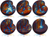Fig. 1. Velocity fields Usph in the Runs HD1, RHD1, RHD2 (top row from left to right), and RHD3, RHD4, and RHD5 (bottom row). The colour contours indicate the radial velocity $U_r^{\mathrm{sph}}$ and the streamlines are colour coded according to the local value of $U_r^{\mathrm{sph}}$.

Fig. 2. Same as Fig. 1 but for run MHD5.

The statistically stationary horizontally averaged thermodynamic state from the non-rotating run HD1 is shown in Fig. 3a. The temperature varies by an order of magnitude within the star whereas the density varies by a factor of roughly 20. This corresponds to roughly five pressure or three density scale heights, respectively. In the exterior of the star the temperature is nearly constant and the density decreases there exponentially as a function of radius. In comparison to other similar studies, the density contrast in the current simulations is thus somewhat greater than in Dobler et al. (2006), comparable to that in Brown et al. (2020), and smaller by a factor of a few in comparison to Browning (2008) and Yadav et al. (2015a, 2016).

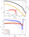Fig. 3. Profiles of mean thermodynamic states from representative runs. Top panel: time-averaged radial profiles of azimuthally averaged temperature $\overline{T}$ (orange, left axis) and density $\overline{\rho }$ (black, right axis) as functions of radius from the non-rotating run HD1. The inset shows the radial profile of the mean specific entropy s̄/cP. Bottom: mean specific entropy s̄/cP(r) from runs HD1, MHD1, MHD3, and MHD5 as indicated by the legend. The dots show a scatter plot of s̄(ϖ,θ) as a function of spherical radius r. The dotted vertical line indicates the upper boundary of the convective layer in the non-rotating run HD1.

The inset of panel a of Fig. 3 shows a scatter plot of the temporally and azimuthally averaged specific entropy s̄(ϖ,z)/c_P. Remarkably, the mean entropy decreases towards the centre of the star below r ≲ 70 Mm. Thus roughly 30% of the core of the star is stably stratified according to the Schwarzschild criterion although the whole star is continuously mixed by vigorous convection. Similar configurations have recently been discussed in other contexts, in which the star has a clearly defined radiative core (e.g., Tremblay et al. 2015; Käpylä et al. 2017a, 2019; Bekki et al. 2017). Such formally stable, yet convecting, regions are thought to arise due to cool plumes originating near to the surface penetrating deep into the stellar interior and regions that would otherwise be convectively stable. This process is sometimes referred to as cool entropy rain (e.g., Brandenburg 2016). The idea of such surface-driven stellar convection goes back to the studies of Stein & Nordlund (1989) and Spruit (1997). Theoretically, the energy transport in such stably stratified but still convective layers is explained by a non-local, non-gradient contribution to the heat flux (Deardorff 1961, 1966). These regions are referred to as Deardorff zones (see, e.g., Brandenburg 2016; Käpylä et al. 2017a). The significance of Deardorff zones in fully convective stars is that they can have an impact on the large-scale dynamos in that the magnetic fields are less susceptible to be buoyant in the possibly stably stratified core.

Figure 3b shows further that in run MHD1 the convective layer is unstably stratified throughout whereas in run MHD3 the Deardorff layer reappears. The behaviour of run MHD1 is puzzling and possibly related to the strong anti-solar differential rotation developing in that run. In the most rapidly rotating case, MHD5, the stratification is again unstable throughout. This can be understood in terms of an increasing critical Rayleigh number as the rotation increases such that a steeper temperature gradient is needed to drive convection (e.g., Chandrasekhar 1961). The current simulations were made with rather modest Rayleigh numbers (see Col. 8 in Table 1) and the effects of rotation are likely to be much weaker in real stars, for which the Rayleigh numbers are more than ten orders of magnitude greater. Figure 3b also shows that the latitudinal variation of mean specific entropy increases as a function rotation indicated by the larger scatter around the horizontally averaged means.

The luminosities related to the radiative, enthalpy, kinetic energy, cooling and heating fluxes are given by

$$\begin{array}{cc}& {\overline{L}}_{\mathrm{rad}}=-4\pi r^2{⟨K⟩}_{\theta \varphi t}\frac{\partial {⟨T⟩}_{\theta \varphi t}}{\partial r},\hfill \end{array}$$(31)

$$\begin{array}{cc}& {\overline{L}}_{\mathrm{enth}}=4\pi r^2{c}_{\mathrm{P}}{⟨{(\rho U_r^{\mathrm{sph}})}^{\prime }{T}^{\prime }⟩}_{\theta \varphi t},\hfill \end{array}$$(32)

$$\begin{array}{cc}& {\overline{L}}_{\mathrm{kin}}=2\pi r^2{⟨\rho {\mathit{U}}^2{U}_r^{\mathrm{sph}}⟩}_{\theta \varphi t},\hfill \end{array}$$(33)

$$\begin{array}{cc}& {\overline{L}}_{\mathrm{visc}}=-8\pi r^2\nu {⟨\rho U_i^{\mathrm{sph}}{\mathsf{S}}_{\mathit{ir}}^{\mathrm{sph}}⟩}_{\theta \varphi t},\hfill \end{array}$$(34)

$$\begin{array}{cc}& {\overline{L}}_{\mathrm{cool}}=-{\displaystyle {\int }_0^r}4\pi r^2{⟨\mathcal{C}⟩}_{\theta \varphi t}\mathrm{d}r,\hfill \end{array}$$(35)

$$\begin{array}{cc}& {\overline{L}}_{\mathrm{heat}}={\displaystyle {\int }_0^r}4\pi r^2{⟨\mathcal{H}⟩}_{\theta \varphi t}\mathrm{d}r,\hfill \end{array}$$(36)

where the primes indicate fluctuations from an azimuthally averaged mean. Furthermore, the total convected luminosity is given by Cattaneo et al. (1991)

$$\begin{array}{c}\hfill {\overline{L}}_{\mathrm{conv}}={\overline{L}}_{\mathrm{enth}}+{\overline{L}}_{\mathrm{kin}}.\end{array}$$(37)

The dominant contributions to the total luminosity from Eqs. (31) to (36) from the non-rotating hydrodynamic run HD1 are shown in Fig. 4. The luminosities due to viscous and radiative fluxes are less than one per cent of the total everywhere and therefore they are not shown. The radiative flux is likely underestimated in the current simulations owing to a value of K₀ that is smaller than that corresponding to an M5 dwarf with the used L_ratio. The effect of this is that the convective velocities in the simulations are somewhat higher than in the target star. Assessing the effect of this for the resulting flows and dynamos is postponed to future studies. The dominant components are due to the outward enthalpy flux (${\overline{L}}_{\mathrm{enth}}$) and the inward kinetic energy flux (${\overline{L}}_{\mathrm{kin}}$). The maximum value of the latter is close to the stellar luminosity, which is compensated by a correspondingly higher flux of enthalpy such that the total convected luminosity ${\overline{L}}_{\mathrm{conv}}$ matches the luminosity of the star everywhere except near to the surface where the cooling is effective. In the rotating cases the enthalpy and kinetic energy luminosity contributions decrease, while they still transport the majority of the flux similar to the fully convective models of Brown et al. (2020).

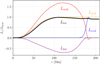Fig. 4. Contributions to the luminosity from enthalpy (red), kinetic energy (purple), cooling (blue), and heating (orange) fluxes in run HD1.

3.2. Large-scale flows

The density-stratified and rotating convective envelopes of fully convective stars have all the ingredients for generating large-scale mean flows via the Λ effect (e.g., Rüdiger 1980, 1989; Käpylä 2019b). The ensuing differential rotation and meridional circulation are of prime importance for large-scale dynamos. Simulations in spherical shells indicate that two qualitatively different flow regimes exist depending on the Coriolis number. For slow rotation the differential rotation is anti-solar, such that the equatorial rotation rate is slower than the polar rate, whereas for rapid rotation a solar-like rotation profile with equatorial acceleration is obtained (e.g., Gilman 1977; Aurnou et al. 2007; Käpylä et al. 2011; Guerrero et al. 2013; Gastine et al. 2014). The watershed value of the Coriolis number in such simulations is close to unity (e.g., Gastine et al. 2014).

The averaged rotation rate is given by

$$\begin{array}{c}\hfill \overline{\mathrm{\Omega }}(\varpi ,z)={\mathrm{\Omega }}_0+{\overline{U}}_{\varphi }(\varpi ,z)/\varpi .\end{array}$$(38)

Similarly, the averaged meridional flow is given by

$$\begin{array}{c}\hfill {\overline{\mathit{U}}}_{\mathrm{mer}}(\varpi ,z)=({\overline{U}}_{\varpi },0,{\overline{U}}_z),\end{array}$$(39)

where the velocities correspond to those in cylindrical coordinates. Both $\overline{\mathrm{\Omega }}$ and ${\overline{\mathit{U}}}_{\mathrm{mer}}$ are averaged in time over the statistically steady part of the simulations. The averaging periods are listed in Col. 12 of Table 1. The amplitude of the differential rotation is measured by the differential rotation parameters (e.g., Käpylä et al. 2013):

$$\begin{array}{cc}& {\mathrm{\Delta }}_{\mathrm{\Omega }}^{(r)}=\frac{\overline{\mathrm{\Omega }}(r_{\mathrm{top}},{\theta }_{\mathrm{eq}})-\overline{\mathrm{\Omega }}(r_{\mathrm{bot}},{\theta }_{\mathrm{eq}})}{\overline{\mathrm{\Omega }}(r_{\mathrm{top}},{\theta }_{\mathrm{eq}})},\hfill \end{array}$$(40)

$$\begin{array}{cc}& {\mathrm{\Delta }}_{\mathrm{\Omega }}^{(\overline{\theta })}(\theta )=\frac{\overline{\mathrm{\Omega }}(r_{\mathrm{top}},{\theta }_{\mathrm{eq}})-\overline{\mathrm{\Omega }}(r_{\mathrm{top}},\overline{\theta })}{\overline{\mathrm{\Omega }}(r_{\mathrm{top}},{\theta }_{\mathrm{eq}})},\hfill \end{array}$$(41)

where r_top = 0.9R, r_bot = 0.1R, θ_eq = 0° corresponds to the equator, and $\overline{\theta }$ refers to an average of $\overline{\mathrm{\Omega }}$ from latitudes +θ and −θ. Table 2 summarizes the results for ${\mathrm{\Delta }}_{\mathrm{\Omega }}^{(r)}$ and ${\mathrm{\Delta }}_{\mathrm{\Omega }}^{(\overline{\theta })}$ with θ = 60° and 75°. The reason not to use the surface velocities for measuring the differential rotation is that the values at r = R are likely to be affected by the damping of velocities applied in the exterior. Similarly, the values near to the axis are the most uncertain and thus off-axis and off-pole values for ${\mathrm{\Delta }}_{\mathrm{\Omega }}^{(r)}$ and ${\mathrm{\Delta }}_{\mathrm{\Omega }}^{(\overline{\theta })}$ are used.

Figure 5 shows the rotation profiles of the runs in the set MHD. The case with the slowest rotation (MHD1), where P_rot = 433 d and Co = 0.7, shows anti-solar differential rotation. This is described by negative values of ${\mathrm{\Delta }}_{\mathrm{\Omega }}^{(r)}$ and ${\mathrm{\Delta }}_{\mathrm{\Omega }}^{(\overline{\theta })}$ (see Row 6 of Table 2). The anti-solar rotation profile is associated with a single-cell anticlockwise meridional flow pattern with outward flow at the equator. This is similar to runs 2b and 2c of Dobler et al. (2006); see their Fig. 11. The amplitude of the meridional flow is relatively large (about 4 m s⁻¹), which corresponds to 20% of the overall rms velocity. These results coincide qualitatively with simulations of thinner convective shells in spherical coordinates (e.g., Käpylä et al. 2014). In run MHD2, where P_rot = 144 d and Co = 2.0, the rotation profile is solar-like with positive ${\mathrm{\Delta }}_{\mathrm{\Omega }}^{(r)}$ and ${\mathrm{\Delta }}_{\mathrm{\Omega }}^{(\overline{\theta })}$ (see Row 7 of Table 2). Thus the transition between anti-solar and solar-like profiles occurs in the Coriolis number range 0.7…2.0. This is slightly lower than in spherical shell convection (e.g., Käpylä et al. 2011; Gastine et al. 2014; Viviani et al. 2018), where the transition typically occurs somewhere between Co = 2…3. However, owing to the differences in the set-ups including the geometry, Prandtl numbers, spatial resolution, and Reynolds and Péclet numbers there is no reason to expect that the transition would occur precisely at the same Co. Nevertheless, it is safe to conclude that the anti-solar to solar-like transition occurs at a similar rotational influence in fully and partially convective models.

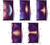Fig. 5. Temporally and azimuthally averaged rotation profiles $\overline{\mathrm{\Omega }}(\varpi ,z)$ for the simulations in set MHD. The values for runs MHD4 and MHD5 are clipped to highlight features near to the equator. The full ranges are indicated in the parenthesis above and below the colour bar. The arrows indicate the mass flux due to meridional circulation $\overline{\rho }{\overline{\mathit{U}}}_{\mathrm{mer}}$. The arrow widths are proportional to $|\overline{\rho }{\overline{\mathit{U}}}_{\mathrm{mer}}|$. The maximum meridional flow speeds are indicated in the bottom right corners of each panel.

The amplitudes of the differential rotation are the largest in the cases MHD1 and MHD2 (see Rows 6 and 7 of Table 2). A comparison of ${\mathrm{\Delta }}_{\mathrm{\Omega }}^{(r)}$ and ${\mathrm{\Delta }}_{\mathrm{\Omega }}^{(\overline{\theta })}$ with Fig. 5 indicates that the latter somewhat exaggerates the amplitude of the differential rotation for these runs because the highest values of $\overline{\mathrm{\Omega }}$ in both cases occur in small regions near to the axis where the accuracy of the ϕ averages is the poorest. Nevertheless, the amplitude of the differential rotation is substantially larger in these two runs in comparison to the more rapidly rotating cases, although the fraction of the kinetic energy in the mean flows in the latter is relatively low; see Cols. 2–4 of Table 3. The rotation profile of run MHD2 is also asymmetric with respect to the equator. This is most likely caused by the asymmetric large-scale magnetic field configuration in that simulation (see below). Similar asymmetric large-scale flow and magnetic field configurations were reported in Dobler et al. (2006); see their Fig. 11. Furthermore, asymmetry is absent in the corresponding hydrodynamic run RHD2 (not shown). The meridional flow pattern in run MHD2 consists of four (two) cells near to (away from) the rotation axis. The meridional flow is also asymmetric near to the equator with maximum flow speeds of the order of 3 m s⁻¹. Comparison between runs MHD[1-2] with corresponding hydrodynamic runs RHD[1-2] shows a reduction of differential rotation of roughly 20%, except for ${\mathrm{\Delta }}_{\mathrm{\Omega }}^{(r)}$ in run MHD1, which is reduced by more than 50%.

In run MHD3 the rotation profile is similar to that in MHD2, but no equatorial asymmetry is present (see Fig. 5). In MHD3 and the more rapidly rotating cases the maximum meridional circulation amplitudes occur outside the star and the flows within the star are significantly weaker. However, as shown in Fig. 5, the mass flux due to these exterior flows is weak because of the rapidly decreasing density for r > R. The values of ${\mathrm{\Delta }}_{\mathrm{\Omega }}^{(r)}$ and ${\mathrm{\Delta }}_{\mathrm{\Omega }}^{(\overline{\theta })}$ in runs MHD[2-3] are similar to those of the Sun. However, magnetic quenching of differential rotation in run MHD3 in comparison to the corresponding hydrodynamic run RHD3 is stronger than for runs MHD2/RHD2. This is likely explained by the stronger magnetic fields in run MHD3 in comparison to MHD2; see Col. 5 of Tables 1 and 3.

In the two most rapidly rotating runs (MHD4 and MHD5) the amplitude of the differential rotation decreases further such that in the latter run the deviations from solid body rotation are very small; see the bottom Row of Fig. 5 and Rows 11–13 in Table 2. The meridional flow also decreases and the largest values are always found outside of the star in both cases. The rotation profile shows axially aligned structures consistent with the Taylor–Proudman balance in run MHD3, but a similar dominance is not as clear from the mean flows in cases MHD4 and MHD5. This is possibly because the mean flows are weak in both cases such that these models are nearly in solid body rotation. This is expected because for rapid enough rotation, turbulent angular momentum transport, and therefore the mean flows, are quenched such that the system approaches solid body rotation for Ω₀ → ∞ (e.g., Kichatinov & Rüdiger 1993; Gastine et al. 2014). However, inspection of instantaneous velocity fields reveals flow structures that are very much in line with Taylor–Proudman constraint (see also Figs. 1 and 2). The higher resolution MHDh simulations do not qualitatively differ from their lower resolution counterparts. The overall kinetic energy in the MHDh runs is slightly lower than in the corresponding MHD runs. A similar trend is seen for ${\mathrm{\Delta }}_{\mathrm{\Omega }}^{(r)}$ and ${\mathrm{\Delta }}_{\mathrm{\Omega }}^{(\overline{\theta })}(\theta )$ for runs MHD1h and MHD3h. This is likely due to the stronger magnetic fields in the MHDh runs (see Tables 1 and 3).

The simulations reported in Dobler et al. (2006) all have anti-solar differential rotation. The Coriolis numbers were not given in that study, but it is possible to calculate Co according to Eq. (26) with the data presented in the paper. See Appendix A for more details regarding quantitative comparisons to the study of Dobler et al. (2006) and how to transform quantities between code and physical units. The Coriolis numbers for their runs 2[b-e] are 0.9, 4.9, 18, and 47; see Table A.1. Based on these values it is somewhat surprising that the differential rotation is anti-solar in their most rapidly rotating cases. However, the rotation profiles in Dobler et al. (2006) are shown from the saturated dynamo regime, where the magnetic field has a considerable back-reaction to the flow. Furthermore, in the most rapidly rotating cases the supercriticality of convection is likely to be even weaker than in the present simulations. Thus it is plausible that the two most rapidly rapidly rotating cases (2d and 2e) in Dobler et al. (2006) are comparable to the current runs MHD4 and MHD5 with weak differential rotation in general.

The rotation profiles of all runs with solar-like rotation profiles (MHD[2–5]) all have multiple meridional circulation cells. This is independent of magnetic fields because the corresponding hydrodynamic runs have qualitatively similar meridional flow structure. On the other hand, mean-field models of fully convective stars, relying on parameterization of turbulence in terms of turbulent viscosity and Λ effect (Pipin 2017; Pipin & Yokoi 2018) almost invariably produce a single-cell meridional circulation pattern. On the other hand, the amplitude of the differential rotation in the P_rot = 10 d model of Pipin (2017) is very close to that in run MHD4.

3.3. Dynamo solutions

All of the runs in sets MHD and MHDh produce large-scale dynamos starting from a low amplitude (∼1 G) random small-scale seed field. Representative instantaneous magnetic fields from runs MHD[1–5] are shown in Fig. 6. While the slowly rotating cases MHD[1–2] do not appear to show large-scale order at a first glance, the more ordered large-scale structure of the magnetic field in the intermediate and rapidly rotating cases MHD[3–5] is immediately clear. Using the same seed field in the non-rotating run HD1 leads to a decaying solution such that there is no small-scale dynamo in that case (run MHD0).

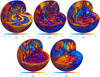Fig. 6. Instantaneous magnetic fields Bsph in the runs MHD1, MHD2, MHD3 (top row from left to right), MHD4, and MHD5 (bottom row). The colour contours indicate radial magnetic field $B_{\mathrm{\varphi }}^{\mathrm{sph}}$ and the streamlines are colour coded according to the local value of $B_{\mathrm{\varphi }}^{\mathrm{sph}}$.

The mean field is considered to be the azimuthally averaged field $\overline{\mathit{B}}(r,\theta ,t)$ or $\overline{\mathit{B}}(\varpi ,z,t)$. Space-time diagrams of B̅_ϕ(R,θ,t) for a period of 100 years for each of the MHD runs are shown in Fig. 7. The model with the slowest rotation (MHD1, P_rot = 430 days) produces a quasi-stationary large-scale field without sign reversals during the simulated period. This is similar to results obtained from spherical wedges and fully spherical shells in the slowly rotating regime in which differential rotation is anti-solar (Käpylä et al. 2017b; Warnecke 2018; Strugarek et al. 2018). A similar quasi-stationary solution is also obtained in case MHD2 that has solar-like differential rotation. Similar quasi-stationary configurations have also been reported from spherical shells with solar-like differential rotation (e.g., Brown et al. 2010; Guerrero et al. 2016) along with solutions with apparently random sign reversals (e.g., Fan & Fang 2014; Hotta et al. 2016). This type of solutions appears to be the norm in a parameter regime, in which the Coriolis number is just high enough for solar-like differential rotation to appear (e.g., Warnecke 2018). Intriguingly, the kinetic helicity, $\mathcal{H}=\overline{\mathit{\omega }·\mathit{U}}$, in these runs shows a profile with a mostly positive (negative) values in the upper part of the CZ in the northern (southern) hemisphere (see the left panel of Fig. 8). This is at odds with the usual argumentation for helical convective eddies in a stratified atmosphere for which ℋ <  0 for $\mathit{g}·\overline{\mathbf{\Omega }}<0$. However, qualitatively similar results have been reported from a slowly rotating fully convective set-up in the context of proto-neutron stars (Masada et al. 2020).

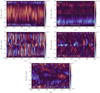Fig. 7. Time-latitude diagrams of the mean toroidal magnetic field B̅ϕ(R,t) for a period of 100 yr for the MHD runs as indicated by the legends. The dotted horizontal line indicates the equator.

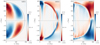Fig. 8. Azimuthally averaged normalized kinetic helicity $\stackrel{\sim }{\mathcal{H}}(\varpi ,z)=\mathcal{H}(\varpi ,z)/u_{\mathrm{rms}}{\omega }_{\mathrm{rms}}$ for runs MHD1 (left), MHD3 (middle), and MHD5 (right). The data ranges are clipped for better legibility. The full ranges are indicated above and below the colour bars.

In the intermediate rotation regime (run MHD3), where P_rot = 43 d and Co = 9.1, a predominantly axisymmetric and oscillatory solution is found. In this regime the rotation profile of the star is solar-like such that the radial gradient of $\overline{\mathrm{\Omega }}$ is positive almost everywhere. In combination with a mostly negative kinetic helicity on the northern hemisphere the expectation from a simple αΩ dynamo is that a poleward-propagating dynamo wave appears (Parker 1955; Yoshimura 1975). This is consistent with the outcome of the simulation (see the left panel in the middle row of Fig. 7), although the kinetic helicity is negative only near to the surface of the star (middle panel of Fig. 8). However, the results for the large-scale magnetic fields agree with comparable simulations in spherical shells (e.g., Gilman 1983; Käpylä et al. 2010; Brown et al. 2011; Simitev et al. 2015). The evolution of the azimuthally averaged mean magnetic field in the course of the cycle is shown in Fig. 9. The amplitude of the mean toroidal magnetic field is typically larger than the corresponding poloidal field, but the difference is not particularly large and in some instances the maximum poloidal field exceeds the maximum toroidal field. However, the volume- and time-averaged toroidal field energy is roughly four times greater than the energy of the poloidal field (see Table 3). Thus the interpretation in terms of an αΩ dynamo remains plausible. However, a more detailed description, for example, in terms of mean-field modelling with turbulent transport coefficients derived from the 3D simulations with the test-field method (e.g., Schrinner et al. 2007; Warnecke et al. 2018; Warnecke & Käpylä 2020) is needed to discern the origin of the large-scale fields. This, however, is not within the scope of the present study.

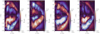Fig. 9. Azimuthally averaged toroidal (colour contours) and poloidal (arrows) magnetic fields from four times between t = 143.4 and 152 yr in run MHD3. The width of the arrows is proportional to the strength of the poloidal field. The values of B̅ϕ are clipped to ±12 kG, and maximum and minimum values are quoted in parenthesis above and below the colour-bar ranges, respectively. The amplitude of the poloidal field is indicated in the bottom right corner of each panel.

In a recent study, Yadav et al. (2016) presented a spherical shell simulation extending from r = 0.1R to R in a parameter regime specifically targeting the slowly rotating M dwarf Proxima Centauri where P_rot ≈ 90 d. These authors found a similar poleward-propagating dynamo wave as in the current run MHD3 with a half-cycle period of roughly nine years. The run MHD3 with P_rot = 43 d has an average half-cycle of around four to five years. Although the parameters of the current simulations and those of Yadav et al. (2016) do not fully overlap, the comparison suggests that neglecting a small core region at the centre of the star does not play a crucial role in the dynamo solution. Furthermore, these numerical findings are close to recent observational results that suggest an activity cycle of about seven years for Proxima Centauri (Suárez Mascareño et al. 2016; Wargelin et al. 2017; Klein et al. 2021).

In another recent study, Brown et al. (2020) report on a simulation of a fully convective star in the rapidly rotating regime. These authors quote a vorticity-based Rossby number Ro = |∇ × u|/2Ω ≈ 0.3 and a velocity-based Rossby number Ro_u = |u|/2ΩR ≈ 0.01, where $\mathit{u}=\mathit{U}-\overline{\mathit{U}}$ is the fluctuating velocity, for this simulation. The inverses of the velocity- and vorticity-based Coriolis numbers of the current study, 1/Co and 1/Co^(ω), are not exactly the same as the Rossby numbers of Brown et al. (2020) because they are based on the total velocity U and thus overestimate the Rossby number by some factor. Thus the Ro of the simulation presented Brown et al. (2020) is most likely somewhere between the current runs MHD3 and MHD4, where 1/Co^(ω) = 0.27 and 1/Co^(ω) = 0.83. The ratio E_mag/E_kin is also comparable to that quoted by Brown et al. (2020) (0.25) in runs MHD3 (0.17) and MHD3h (0.27).

These authors found a dynamo solution that is predominantly hemispheric. Furthermore, they explain that similar solutions are found in the parameter regime in the vicinity of the reported simulation. The current simulations do not indicate a similar behaviour but sweeping conclusions cannot be made based on the very limited number of simulations done so far. There are some periods in run MHD3 where the magnetic field is predominantly hemispherical (see Fig. 10), but such configurations cover only a small fraction of the total duration of the simulation. Furthermore, the mean magnetic field in run MHD2 is consistently stronger on the southern hemisphere (see Fig. 7). This is perhaps suggesting that oscillatory hemispheric solutions could also be realized for parameters not far away from those in the present runs MHD2 and MHD3. Another example of a possibly hemispheric dynamo was presented by Browning (2008) with velocity fluctuation-based Rossby number of ≈10⁻², but there is not enough information regarding the time evolution of the magnetic fields to ascertain this definitively (see their Fig. 7 panels b and c).

Fig. 10. Same as Fig. 9 but for t = 123.1 (left) and t = 155.6 yr (right).

For the rapid rotators (runs MHD4 and MHD5) the axisymmetric magnetic fields show no clear cycles while the mean fields appear to migrate predominantly towards the equator (Fig. 7). However, the fraction of the axisymmetric mean field energy in comparison to the total field energy sharply decreases in runs MHD[4–5] in comparison to intermediate rotation cases; see Cols. 7 and 8 of Table 3. This is, however, associated with a strong increase in the total magnetic energy (Col. 5 of Table 3), and a closer inspection indicates that the magnetic fields in these cases have a strong non-axisymmetric contribution with a dominant m = 1 mode; see representative results from MHD5 in Fig. 11. This large-scale non-axisymmetric structure also drifts with respect to the rotating frame of the star. Such azimuthal dynamo waves were predicted by mean-field theory (Krause & Rädler 1980) and have more recently been reported from simulations of stellar dynamos (e.g., Käpylä et al. 2013; Cole et al. 2014; Yadav et al. 2015b; Viviani et al. 2018; Navarrete et al. 2021). In run MHD4 (MHD5) the m = 1 magnetic structure drifts in the retrograde direction with a period of roughly 10 (40) years. These periods are also similar to those in simulations of rapidly rotating solar-like stars (e.g., Cole et al. 2014; Viviani et al. 2018).

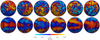Fig. 11. Magnetic field Bsph at r = R in run MHD5 from six snapshots separated by roughly 6 years each. Top (bottom) row: magnetic fields pole-on (equator-on). The colour contours and the colour coding of the field lines indicate strength of the local radial field. The colour scale is clipped at ±16 kG and the extrema of $B_r^{\mathrm{sph}}$ are ±70 kG.

The rightmost panel of Fig. 8 shows that the kinetic helicity is mostly negative on the northern hemisphere in run MHD5, although the normalized values are smaller than in the less rapidly rotating cases. Owing to the almost totally absent differential rotation, the most plausible dynamo mechanism in this case is an α² dynamo. However, more detailed information concerning the turbulent transport coefficients are needed to confirm this.

The higher resolution runs in the MHDh set of simulations do not show qualitative differences from the corresponding lower resolution simulations MHD[1,3,5]. The overall magnetic field strength is higher in the MHDh runs by 15 (MHD1h) to 40 (MHD5h) per cent. Nevertheless, the spatial structure and temporal evolution of the large-scale magnetic fields are similar to those in the lower resolution runs in set MHD. Therefore the results appear to be robust although higher resolution studies are still needed to study effects such as efficient small-scale dynamo action and larger density stratifications.

The rms field strengths in the current runs exceed 10 kG in all cases except MHD2; see Col. 5 of Table 1. Furthermore, the order of magnitude of the magnetic energies (10⁵ J m⁻³; see Col. 5 of Table 3) in the current runs agrees with Browning (2008), suggesting similar field strengths and that the results are robust irrespective of the numerical method. Magnetic fields exceeding 10 kG are somewhat higher than those observed in M dwarfs, for which typical total field strengths are of the order of a few kilogauss (e.g., Kochukhov 2021, and references therein). There are several possible reasons for the apparent discrepancy, including a too low resolution of the simulations or the observations. A possible way forward is to produce synthetic observations, such as coarse-grained maps of surface fields (e.g., Yadav et al. 2015a) or time series corresponding to brightness variations, from the simulation results and comparing those with actual observations. This will be addressed in future work.

4. Conclusions

An updated version of the star-in-a-box model originally published by Dobler et al. (2006) was used to compute hydrodynamic and MHD models of a 0.2 M_⊙ fully convective M5 star with various rotation rates. The current results indicate that the transition from anti-solar to solar-like differential rotation in fully convective stars occurs at a comparable rotational regime, as measured by a Coriolis number, as in simulations of partially convective stars (e.g., Gastine et al. 2014; Käpylä et al. 2014). Furthermore, the dynamo-generated, large-scale magnetic fields are predominantly axisymmetric and quasi-stationary for slow rotation and axisymmetric and cyclic for intermediate rotation. For rapid rotation the large-scale fields become increasingly non-axisymmetric with a dominating low-order (m = 1) mode. These large-scale non-axisymmetric fields also exhibit azimuthal dynamo waves where the large-scale magnetic structure drifts in longitude with little regard of the underlying flows (e.g., Krause & Rädler 1980; Cole et al. 2014). Remarkably, very similar transitions at comparable Coriolis numbers have been reported from spherical shell simulations (e.g., Käpylä et al. 2013; Viviani et al. 2018). This suggests that the dynamos in fully convective stars are fundamentally the same as in partially convective stars.

The current exploratory set of simulations presented in the current study is, however, by no means exhaustive. This is illustrated by the lack of bistable dipolar and multipolar solutions (e.g., Gastine et al. 2013; Yadav et al. 2015a) and hemispheric dynamos (Brown et al. 2020) in the current set of models. A particularly interesting parameter regime is that of intermediate rotation, in the vicinity of the current run MHD3 with P_rot = 43 d, where cyclic dynamo solutions appear. Similar results have been reported from anelastic simulations in spherical shells (Yadav et al. 2016) and in full spheres (Brown et al. 2020). Furthermore, this is also an interesting regime observationally in view of the recent results on the possible activity cycles of Proxima Centauri and Ross 128 with rotation periods of the order of 100 days. Further simulations and comparisons to observations are clearly called for in this range of parameters.

The similarity of the current solutions with the very different numerical approaches of, for example Yadav et al. (2016) and Brown et al. (2020), is encouraging. Although the current results suggest that the highly enhanced luminosity in the current simulations leads to dynamo solutions similar to those achieved in anelastic models, a systematic study of the effects of the luminosity excess is lacking at the moment. Furthermore, degeneracy of stellar matter in M dwarfs is likely to affect the interior thermodynamic structure. While this effect has been neglected in the present study, further research is warranted.

Another aspect that makes fully convective stars interesting is that they are often found in post-common envelope binaries (PCEBs; e.g., Parsons et al. 2013). The periods of many of these binaries show residual signals that indicate orbital evolution of the system. Such signals can be caused by planets although explaining their existence in such evolved systems is a problem in itself. Another explanation is that the secondary star hosts a cyclic dynamo that affects the gravitational quadrupole moment of the star, which is reflected in orbit variations. This mechanism was first introduced by Applegate (1992) and more recent ideas along similar lines have decreased for example energetic requirements for orbit variations due to non-axisymmetric, large-scale fields (Lanza 2020). Recent numerical simulations of Navarrete et al. (2020, 2021) demonstrated the effect of dynamo-generated magnetism on the gravitational quadrupole moment for partially convective, rapidly rotating solar-like stars. Extending the study of the stellar quadrupole moment to fully convective stars is a logical step to follow in future publications.

Acknowledgments

I thank the anonymous referee, Axel Brandenburg, Fabio del Sordo, Oleg Kochukhov, Felipe Navarrete, Carolina Ortiz, Günther Rüdiger, Dominik Schleicher, and Jörn Warnecke for fruitful discussions and useful comments on the manuscript. I acknowledge the hospitality of Nordita during my visit in February-March 2020. The simulations were made using the HLRN-IV supercomputers Emmy and Lise hosted by the North German Supercomputing Alliance (HLRN) in Göttingen and Berlin, Germany. This work was supported by the Deutsche Forschungsgemeinschaft Heisenberg programme (grant No. KA 4825/2-1).

References

Appendix A: Comparison to Dobler et al. (2006)

Since the simulations of Dobler et al. (2006) were made with the same model as in the current study, it is possible to make direct quantitative comparisons of the parameters and results. Using the values of ℒ and other parameters quoted in Table 1 of Dobler et al. (2006) it is possible to compute the outputs of the model in physical units. A number of such outputs, along with a few dimensionless numbers transformed to the same definitions as in the present study are listed in Table A.1.

The conversion factor between the rotation rates in the simulation and the target star was given in Eq. (21). For all of the runs of Dobler et al. (2006) except 1c this yields

$$\begin{array}{c}\hfill {\mathrm{\Omega }}_{\odot }^{\mathrm{sim}}=12.5{\left(\frac{g^{\mathrm{sim}}}{R^{\mathrm{sim}}}\right)}^{1/2},\end{array}$$(A.1)

for the solar rotation rate Ω_⊙ = 2.7 × 10⁻⁶ s⁻¹. For their run 1c the prefactor is 10.1 instead of 12.5. In the most rapidly rotating run of Dobler et al. (2006) the rotation rate is Ω₀ = 10(g^sim/R^sim)^1/2, where g^sim = R^sim = 1 in code units. This means that the rotation period in that run is still more than 30 d; see Cols. 4 and 5 of Table A.1. Nevertheless, this run is in the rapidly rotating regime because of the overall lower convective velocities than in the present study; compare Col. 4 of Table 1 with Col. 6 of Table A.1. This is most clearly seen in their non-rotating case 2a, where u_rms = 9.3 m s⁻¹, whereas u_rms = 18 m s⁻¹ in the current run HD1. Such lower velocities are likely due to the more efficient radiative energy transport in their runs. That is, convection transports only a fraction of the energy instead of practically the whole luminosity as in the present study.

The conversion of velocities and magnetic fields from simulation to physical units is done through (cf. Appendix A of Käpylä et al. 2020)

$$\begin{array}{cc}& {\mathit{U}}^{\mathrm{phys}}=\left(\frac{{\mathrm{\Omega }}_{\odot }R}{{\mathrm{\Omega }}_{\odot }^{\mathrm{sim}}{R}^{\mathrm{sim}}}\right){\mathit{U}}^{\mathrm{sim}},\hfill \end{array}$$(A.2)

$$\begin{array}{cc}& {\mathit{B}}^{\mathrm{phys}}={\left[\frac{{\mu }_0{\rho }_0{({\mathrm{\Omega }}_{\odot }R)}^2}{{\mu }_0^{\mathrm{sim}}{\rho }_0^{\mathrm{sim}}{({\mathrm{\Omega }}_{\odot }^{\mathrm{sim}}{R}^{\mathrm{sim}})}^2}\right]}^{1/2}{\mathit{B}}^{\mathrm{sim}},\hfill \end{array}$$(A.3)

where ${\mu }_0^{\mathrm{sim}}={\rho }_0^{\mathrm{sim}}=1$ are used in the code, and where the solar rotation rate is used as a reference value.

The Reynolds numbers in Dobler et al. (2006) were computed using the stellar radius R as the length scale whereas the corresponding wave number k_R = R/2π is used in the definitions in the present study. Thus the fluid and magnetic Reynolds numbers with the current definitions in Eq. (28) are written as

$$\begin{array}{c}\hfill \mathrm{Re}=\frac{{\mathrm{Re}}^{\mathrm{DSB}}}{2\pi },{\mathrm{Re}}_{\mathrm{M}}=\frac{{\mathrm{Re}}_{\mathrm{M}}^{\mathrm{DSB}}}{2\pi },\end{array}$$(A.4)

where the superscript DSB refers to the definitions in Dobler et al. (2006). Furthermore, the Péclet number can be computed using the quantities given in Table 1 of Dobler et al. (2006). We note that a constant χ was used by Dobler et al. (2006) and no SGS entropy diffusion is added. Finally, the Coriolis number according to Eq. (26) is given by

$$\begin{array}{c}\hfill \mathrm{Co}=\frac{{\mathrm{\Omega }}_0{R}^2}{\nu \pi {\mathrm{Re}}_{\mathrm{DSB}}}·\end{array}$$(A.5)

Even though the rotation rates of the runs in Dobler et al. (2006) are lower, the Coriolis numbers are comparable to those in the present study. The fluid Reynolds numbers are generally smaller by a factor of roughly three, while the magnetic Reynolds numbers are somewhat higher in Dobler et al. (2006). This explained by the higher magnetic Prandtl number (Pm = 2) in comparison to the present study (Pm = 0.5). This also explains why a small-scale dynamo is excited in run 2a of Dobler et al. (2006) with Re_M = 93, while it is absent in the current run MHD0 with an almost identical magnetic Reynolds number (Re_M = 95) (see e.g., Schekochihin et al. 2007; Käpylä et al. 2018).

All Tables

All Figures

	Fig. 1. Velocity fields Usph in the Runs HD1, RHD1, RHD2 (top row from left to right), and RHD3, RHD4, and RHD5 (bottom row). The colour contours indicate the radial velocity $U_r^{\mathrm{sph}}$ and the streamlines are colour coded according to the local value of $U_r^{\mathrm{sph}}$.
In the text

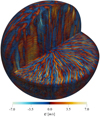	Fig. 2. Same as Fig. 1 but for run MHD5.
In the text

Fig. 3. Profiles of mean thermodynamic states from representative runs. Top panel: time-averaged radial profiles of azimuthally averaged temperature $\overline{T}$ (orange, left axis) and density $\overline{\rho }$ (black, right axis) as functions of radius from the non-rotating run HD1. The inset shows the radial profile of the mean specific entropy s̄/cP. Bottom: mean specific entropy s̄/cP(r) from runs HD1, MHD1, MHD3, and MHD5 as indicated by the legend. The dots show a scatter plot of s̄(ϖ,θ) as a function of spherical radius r. The dotted vertical line indicates the upper boundary of the convective layer in the non-rotating run HD1.

In the text

	Fig. 4. Contributions to the luminosity from enthalpy (red), kinetic energy (purple), cooling (blue), and heating (orange) fluxes in run HD1.
In the text

Fig. 5. Temporally and azimuthally averaged rotation profiles $\overline{\mathrm{\Omega }}(\varpi ,z)$ for the simulations in set MHD. The values for runs MHD4 and MHD5 are clipped to highlight features near to the equator. The full ranges are indicated in the parenthesis above and below the colour bar. The arrows indicate the mass flux due to meridional circulation $\overline{\rho }{\overline{\mathit{U}}}_{\mathrm{mer}}$. The arrow widths are proportional to $|\overline{\rho }{\overline{\mathit{U}}}_{\mathrm{mer}}|$. The maximum meridional flow speeds are indicated in the bottom right corners of each panel.

In the text

	Fig. 6. Instantaneous magnetic fields Bsph in the runs MHD1, MHD2, MHD3 (top row from left to right), MHD4, and MHD5 (bottom row). The colour contours indicate radial magnetic field $B_{\mathrm{\varphi }}^{\mathrm{sph}}$ and the streamlines are colour coded according to the local value of $B_{\mathrm{\varphi }}^{\mathrm{sph}}$.
In the text

	Fig. 7. Time-latitude diagrams of the mean toroidal magnetic field B̅ϕ(R,t) for a period of 100 yr for the MHD runs as indicated by the legends. The dotted horizontal line indicates the equator.
In the text

	Fig. 8. Azimuthally averaged normalized kinetic helicity $\stackrel{\sim }{\mathcal{H}}(\varpi ,z)=\mathcal{H}(\varpi ,z)/u_{\mathrm{rms}}{\omega }_{\mathrm{rms}}$ for runs MHD1 (left), MHD3 (middle), and MHD5 (right). The data ranges are clipped for better legibility. The full ranges are indicated above and below the colour bars.
In the text

Fig. 9. Azimuthally averaged toroidal (colour contours) and poloidal (arrows) magnetic fields from four times between t = 143.4 and 152 yr in run MHD3. The width of the arrows is proportional to the strength of the poloidal field. The values of B̅ϕ are clipped to ±12 kG, and maximum and minimum values are quoted in parenthesis above and below the colour-bar ranges, respectively. The amplitude of the poloidal field is indicated in the bottom right corner of each panel.

In the text

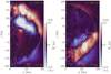	Fig. 10. Same as Fig. 9 but for t = 123.1 (left) and t = 155.6 yr (right).
In the text

	Fig. 11. Magnetic field Bsph at r = R in run MHD5 from six snapshots separated by roughly 6 years each. Top (bottom) row: magnetic fields pole-on (equator-on). The colour contours and the colour coding of the field lines indicate strength of the local radial field. The colour scale is clipped at ±16 kG and the extrema of $B_r^{\mathrm{sph}}$ are ±70 kG.
In the text

References

- Applegate, J. H. 1992, ApJ, 385, 621 [NASA ADS] [CrossRef] [Google Scholar]
- Aurnou, J., Heimpel, M., & Wicht, J. 2007, Icarus, 190, 110 [NASA ADS] [CrossRef] [Google Scholar]
- Baraffe, I., & Chabrier, G. 2018, A&A, 619, A177 [Google Scholar]
- Bekki, Y., Hotta, H., & Yokoyama, T. 2017, ApJ, 851, 74 [NASA ADS] [CrossRef] [Google Scholar]
- Brandenburg, A. 2005, ApJ, 625, 539 [CrossRef] [Google Scholar]
- Brandenburg, A. 2016, ApJ, 832, 6 [Google Scholar]
- Brandenburg, A., Nordlund, A., & Stein, R. F. 2000, in Geophysical and Astrophysical Convection, Contributions from a Workshop Sponsored by the Geophysical Turbulence Program at the National Center for Atmospheric Research, October 1995, eds. P. A. Fox, & R. M. Kerr (The Netherlands: Gordon and Breach Science Publishers), 85 [Google Scholar]
- Brown, B. P., Browning, M. K., Brun, A. S., Miesch, M. S., & Toomre, J. 2010, ApJ, 711, 424 [Google Scholar]
- Brown, B. P., Miesch, M. S., Browning, M. K., Brun, A. S., & Toomre, J. 2011, ApJ, 731, 69 [Google Scholar]
- Brown, B. P., Oishi, J. S., Vasil, G. M., Lecoanet, D., & Burns, K. J. 2020, ApJ, 902, L3 [CrossRef] [Google Scholar]
- Browning, M. K. 2008, ApJ, 676, 1262 [Google Scholar]
- Browning, M. K. 2011, in Astrophysical Dynamics: From Stars to Galaxies, eds. N. H. Brummell, A. S. Brun, M. S. Miesch, & Y. Ponty, IAU Symp., 271, 69 [Google Scholar]
- Brun, A. S., & Palacios, A. 2009, ApJ, 702, 1078 [NASA ADS] [CrossRef] [Google Scholar]
- Carroll, B., & Ostlie, D. 2013, An Introduction to Modern Astrophysics, Pearson Custom library (London: Pearson) [Google Scholar]
- Cattaneo, F., Brummell, N. H., Toomre, J., Malagoli, A., & Hurlburt, N. E. 1991, ApJ, 370, 282 [NASA ADS] [CrossRef] [Google Scholar]
- Chabrier, G., & Baraffe, I. 1997, A&A, 327, 1039 [NASA ADS] [Google Scholar]
- Chabrier, G., & Baraffe, I. 2000, ARA&A, 38, 337 [NASA ADS] [CrossRef] [Google Scholar]
- Chandrasekhar, S. 1961, Hydrodynamic and Hydromagnetic Stability (Cambridge: Cambridge University Press) [Google Scholar]
- Charbonneau, P. 2020, Liv. Rev. Sol. Phys., 17, 4 [Google Scholar]
- Cole, E., Käpylä, P. J., Mantere, M. J., & Brandenburg, A. 2014, ApJ, 780, L22 [NASA ADS] [CrossRef] [Google Scholar]
- Damasso, M., Del Sordo, F., Anglada-Escudé, G., et al. 2020, Sci. Adv., 6 [Google Scholar]
- Deardorff, J. W. 1961, J. Atm. Sci., 18, 540 [Google Scholar]
- Deardorff, J. W. 1966, J. Atm. Sci., 23, 503 [NASA ADS] [CrossRef] [Google Scholar]
- Dikpati, M., & Charbonneau, P. 1999, ApJ, 518, 508 [NASA ADS] [CrossRef] [Google Scholar]
- Dobler, W., Stix, M., & Brandenburg, A. 2006, ApJ, 638, 336 [NASA ADS] [CrossRef] [Google Scholar]
- Donati, J.-F., Morin, J., Petit, P., et al. 2008, MNRAS, 390, 545 [NASA ADS] [CrossRef] [Google Scholar]
- Dorch, S. B. F. 2004, A&A, 423, 1101 [NASA ADS] [CrossRef] [EDP Sciences] [Google Scholar]
- Fan, Y., & Fang, F. 2014, ApJ, 789, 35 [NASA ADS] [CrossRef] [Google Scholar]
- Feiden, G. A., Skidmore, K., & Jao, W.-C. 2021, ApJ, 907, 53 [CrossRef] [Google Scholar]
- Freytag, B., Steffen, M., & Dorch, B. 2002, Astron. Nachr., 323, 213 [Google Scholar]
- Gastine, T., Duarte, L., & Wicht, J. 2012, A&A, 546, A19 [NASA ADS] [CrossRef] [EDP Sciences] [Google Scholar]
- Gastine, T., Morin, J., Duarte, L., et al. 2013, A&A, 549, L5 [NASA ADS] [CrossRef] [EDP Sciences] [Google Scholar]
- Gastine, T., Yadav, R. K., Morin, J., Reiners, A., & Wicht, J. 2014, MNRAS, 438, L76 [Google Scholar]
- Gilman, P. A. 1977, Geophys. Astrophys. Fluid Dyn., 8, 93 [NASA ADS] [CrossRef] [Google Scholar]
- Gilman, P. A. 1983, ApJS, 53, 243 [NASA ADS] [CrossRef] [Google Scholar]
- Guerrero, G., Smolarkiewicz, P. K., Kosovichev, A. G., & Mansour, N. N. 2013, ApJ, 779, 176 [NASA ADS] [CrossRef] [Google Scholar]
- Guerrero, G., Smolarkiewicz, P. K., de Gouveia Dal Pino, E. M., Kosovichev, A. G., & Mansour, N. N. 2016, ApJ, 819, 104 [NASA ADS] [CrossRef] [Google Scholar]
- Hazra, G., Karak, B. B., & Choudhuri, A. R. 2014, ApJ, 782, 93 [NASA ADS] [CrossRef] [Google Scholar]
- Hotta, H., Rempel, M., & Yokoyama, T. 2015, ApJ, 798, 51 [NASA ADS] [CrossRef] [Google Scholar]
- Hotta, H., Rempel, M., & Yokoyama, T. 2016, Science, 351, 1427 [NASA ADS] [CrossRef] [Google Scholar]
- Ibañez Bustos, R. V., Buccino, A. P., Flores, M., & Mauas, P. J. D. 2019, A&A, 628, L1 [CrossRef] [EDP Sciences] [Google Scholar]
- Ibañez Bustos, R. V., Buccino, A. P., Messina, S., Lanza, A. F., & Mauas, P. J. D. 2020, A&A, 644, A2 [CrossRef] [EDP Sciences] [Google Scholar]
- Jao, W.-C., Henry, T. J., Gies, D. R., & Hambly, N. C. 2018, ApJ, 861, L11 [Google Scholar]
- Käpylä, P. J. 2019a, A&A, 631, A122 [CrossRef] [EDP Sciences] [Google Scholar]
- Käpylä, P. J. 2019b, A&A, 622, A195 [NASA ADS] [CrossRef] [EDP Sciences] [Google Scholar]
- Käpylä, P. J., Korpi, M. J., & Tuominen, I. 2006, Astron. Nachr., 327, 884 [CrossRef] [Google Scholar]
- Käpylä, P. J., Korpi, M. J., Brandenburg, A., Mitra, D., & Tavakol, R. 2010, Astron. Nachr., 331, 73 [NASA ADS] [CrossRef] [Google Scholar]
- Käpylä, P. J., Mantere, M. J., & Brandenburg, A. 2011, Astron. Nachr., 332, 883 [NASA ADS] [CrossRef] [Google Scholar]
- Käpylä, P. J., Mantere, M. J., & Brandenburg, A. 2012, ApJ, 755, L22 [NASA ADS] [CrossRef] [Google Scholar]
- Käpylä, P. J., Mantere, M. J., Cole, E., Warnecke, J., & Brandenburg, A. 2013, ApJ, 778, 41 [NASA ADS] [CrossRef] [Google Scholar]
- Käpylä, P. J., Käpylä, M. J., & Brandenburg, A. 2014, A&A, 570, A43 [NASA ADS] [CrossRef] [EDP Sciences] [Google Scholar]
- Käpylä, P. J., Rheinhardt, M., Brandenburg, A., et al. 2017a, ApJ, 845, L23 [NASA ADS] [CrossRef] [Google Scholar]
- Käpylä, P. J., Käpylä, M. J., Olspert, N., Warnecke, J., & Brandenburg, A. 2017b, A&A, 599, A4 [CrossRef] [EDP Sciences] [Google Scholar]
- Käpylä, P. J., Käpylä, M. J., & Brandenburg, A. 2018, Astron. Nachr., 339, 127 [CrossRef] [Google Scholar]
- Käpylä, P. J., Viviani, M., Käpylä, M. J., Brandenburg, A., & Spada, F. 2019, Geophys. Astrophys. Fluid Dyn., 113, 149 [NASA ADS] [CrossRef] [Google Scholar]
- Käpylä, P. J., Gent, F. A., Olspert, N., Käpylä, M. J., & Brandenburg, A. 2020, Geophys. Astrophys. Fluid Dyn., 114, 8 [CrossRef] [Google Scholar]
- Kasting, J. F., Kopparapu, R., Ramirez, R. M., & Harman, C. E. 2014, Proc. Natl. Acad. Sci., 111, 12641 [Google Scholar]
- Kichatinov, L. L., & Rüdiger, G. 1993, A&A, 276, 96 [NASA ADS] [Google Scholar]
- Klein, B., Donati, J.-F., Hébrard, É. M., et al. 2021, MNRAS, 500, 1844 [Google Scholar]
- Kochukhov, O. 2021, A&ARv, 29, 1 [Google Scholar]
- Krause, F., & Rädler, K.-H. 1980, Mean-field Magnetohydrodynamics and Dynamo Theory (Oxford: Pergamon Press) [Google Scholar]
- Lanza, A. F. 2020, MNRAS, 491, 1820 [NASA ADS] [Google Scholar]
- Limber, D. N. 1958, ApJ, 127, 363 [Google Scholar]
- Lin, Y., & Jackson, A. 2021, J. Fluid Mech., 912, A46 [Google Scholar]
- Masada, Y., Takiwaki, T., & Kotake, K. 2020, ApJ, submitted [arXiv:2001.08452] [Google Scholar]
- Morin, J., Donati, J.-F., Petit, P., et al. 2008, MNRAS, 390, 567 [Google Scholar]
- Morin, J., Donati, J.-F., Petit, P., et al. 2010, MNRAS, 407, 2269 [Google Scholar]
- Mullan, D. J., & Houdebine, E. R. 2020, ApJ, 891, 128 [Google Scholar]
- Navarrete, F. H., Schleicher, D. R. G., Käpylä, P. J., et al. 2020, MNRAS, 491, 1043 [Google Scholar]
- Navarrete, F. H., Käpylä, P. J., Schleicher, D. R. G., Ortiz, C. A., & Banerjee, R. 2021, MNRAS, submitted [arXiv:2102.11110] [Google Scholar]
- Nelson, N. J., Brown, B. P., Brun, A. S., Miesch, M. S., & Toomre, J. 2013, ApJ, 762, 73 [Google Scholar]
- O’Mara, B., Miesch, M. S., Featherstone, N. A., & Augustson, K. C. 2016, AdSpR, 58, 1475 [Google Scholar]
- Parker, E. N. 1955, ApJ, 122, 293 [Google Scholar]
- Parsons, S. G., Gänsicke, B. T., Marsh, T. R., et al. 2013, MNRAS, 429, 256 [Google Scholar]
- Pencil Code Collaboration (Brandenburg, A., et al.) 2021, J. Open Source Softw., 6, 2807 [Google Scholar]
- Pipin, V. V. 2017, MNRAS, 466, 3007 [Google Scholar]
- Pipin, V. V., & Kosovichev, A. G. 2011, ApJ, 727, L45 [Google Scholar]
- Pipin, V. V., & Yokoi, N. 2018, ApJ, 859, 18 [Google Scholar]
- Rogachevskii, I., & Kleeorin, N. 2015, J. Plasma Phys., 81, 395810504 [Google Scholar]
- Rüdiger, G. 1980, Geophys. Astrophys. Fluid Dyn., 16, 239 [NASA ADS] [CrossRef] [Google Scholar]
- Rüdiger, G. 1989, Differential Rotation and Stellar Convection. Sun and Solar-type Stars (Berlin: Akademie Verlag) [Google Scholar]
- Schekochihin, A. A., Iskakov, A. B., Cowley, S. C., et al. 2007, New J. Phys., 9, 300 [Google Scholar]
- Schrinner, M., Rädler, K.-H., Schmitt, D., Rheinhardt, M., & Christensen, U. R. 2007, Geophys. Astrophys. Fluid Dyn., 101, 81 [Google Scholar]
- Simitev, R. D., Kosovichev, A. G., & Busse, F. H. 2015, ApJ, 810, 80 [Google Scholar]
- Spruit, H. 1997, Mem. Soc. Astron. It., 68, 397 [Google Scholar]
- Stein, R. F., & Nordlund, A. 1989, ApJ, 342, L95 [Google Scholar]
- Strugarek, A., Beaudoin, P., Charbonneau, P., & Brun, A. S. 2018, ApJ, 863, 35 [Google Scholar]
- Suárez Mascareño, A., Rebolo, R., & González Hernández, J. I. 2016, A&A, 595, A12 [NASA ADS] [CrossRef] [EDP Sciences] [Google Scholar]
- Tremblay, P.-E., Ludwig, H.-G., Freytag, B., et al. 2015, ApJ, 799, 142 [Google Scholar]
- van Saders, J. L., & Pinsonneault, M. H. 2012, ApJ, 751, 98 [Google Scholar]
- Viviani, M., & Käpylä, M. J. 2021, A&A, 645, A141 [EDP Sciences] [Google Scholar]
- Viviani, M., Warnecke, J., Käpylä, M. J., et al. 2018, A&A, 616, A160 [NASA ADS] [CrossRef] [EDP Sciences] [Google Scholar]
- Wargelin, B. J., Saar, S. H., Pojmański, G., Drake, J. J., & Kashyap, V. L. 2017, MNRAS, 464, 3281 [NASA ADS] [CrossRef] [Google Scholar]
- Warnecke, J. 2018, A&A, 616, A72 [NASA ADS] [CrossRef] [EDP Sciences] [Google Scholar]
- Warnecke, J., & Käpylä, M. J. 2020, A&A, 642, A66 [EDP Sciences] [Google Scholar]
- Warnecke, J., Rheinhardt, M., Tuomisto, S., et al. 2018, A&A, 609, A51 [NASA ADS] [CrossRef] [EDP Sciences] [Google Scholar]
- West, A. A., Weisenburger, K. L., Irwin, J., et al. 2015, ApJ, 812, 3 [NASA ADS] [CrossRef] [Google Scholar]
- Woodward, P. R., Lin, P.-H., Mao, H., Andrassy, R., & Herwig, F. 2019, J. Phys. Conf. Ser., 1225, 012020 [Google Scholar]
- Wright, N. J., & Drake, J. J. 2016, Nature, 535, 526 [NASA ADS] [CrossRef] [PubMed] [Google Scholar]
- Wright, N. J., Newton, E. R., Williams, P. K. G., Drake, J. J., & Yadav, R. K. 2018, MNRAS, 479, 2351 [NASA ADS] [CrossRef] [Google Scholar]
- Yadav, R. K., Christensen, U. R., Morin, J., et al. 2015a, ApJ, 813, L31 [NASA ADS] [CrossRef] [Google Scholar]
- Yadav, R. K., Gastine, T., Christensen, U. R., & Reiners, A. 2015b, A&A, 573, A68 [NASA ADS] [CrossRef] [EDP Sciences] [Google Scholar]
- Yadav, R. K., Christensen, U. R., Wolk, S. J., & Poppenhaeger, K. 2016, ApJ, 833, L28 [Google Scholar]
- Yoshimura, H. 1975, ApJ, 201, 740 [Google Scholar]