| Issue |
A&A
Volume 650, June 2021
|
|
|---|---|---|
| Article Number | A189 | |
| Number of page(s) | 26 | |
| Section | Astrophysical processes | |
| DOI | https://doi.org/10.1051/0004-6361/202038795 | |
| Published online | 29 June 2021 | |
Order in the chaos
Eccentric black hole binary mergers in triples formed via strong binary–binary scatterings
1
Astronomisches Rechen-Institut, Zentrum für Astronomie der Universität Heidelberg, Mönchhofstrasse 12-14, Heidelberg 69120, Germany
e-mail: m.arcasedda@gmail.com
2
Center for Relativistic Astrophysics, School of Physics, Georgia Institute of Technology, Atlanta, GA 30332, USA
3
University of Oxford, Rudolf Peierls Centre for Theoretical Physics, Clarendon Laboratory, Parks Road, Oxford OX1 3PU, UK
Received:
30
June
2020
Accepted:
10
April
2021
Black hole (BH) triples represent one of the astrophysical pathways for BH mergers in the Universe detectable by LIGO and VIRGO. We study the formation of BH triples via binary–binary encounters in dense clusters, showing that up to two-thirds of the triples formed through this channel are hierarchical, whereas the remaining one-third are in a non-hierarchical, unstable configuration. We built a database of 32 000 N-body simulations to investigate the evolution of BH triples focusing on mildly hierarchical and non-hierarchical unstable configurations. Varying the mutual orbital inclination, the three BH masses and the inner and outer eccentricities, we show that retrograde, nearly planar configurations lead to a significant shrinkage of the inner binary. We find a universal trend of triple systems, namely that they tend to evolve toward prograde configurations and that the orbital flip, driven by the torque exerted on the inner BH binary (BHB) by the outer BH, leads in general to tighter inner orbits. In some cases, the resulting BHB undergoes coalescence within a Hubble time, releasing gravitational waves. A large fraction of merging BHBs with an initial separation of 1 AU enter the 10−3 − 10−1 Hz frequency band with large eccentricities, thus representing potential eccentric LISA sources. Mergers originating from an initially tighter BHB (a ∼ 0.01 AU), instead often have eccentricities above 0.7 in the 1 Hz band. We find that the mass distribution of the mergers in this astrophysical channel maps the original BH binary spectrum. This might have interesting consequences in light of the growing population of BH mergers detected by LIGO and VIRGO, namely that eccentric sources detected in high-frequency detectors are most likely connected with a high-velocity dispersion stellar environment, whereas eccentric sources detected in low-frequency detectors are likely to develop in low-density clusters.
Key words: stars: black holes / stars: kinematics and dynamics / galaxies: star clusters: general / black hole physics / gravitation / methods: numerical
© ESO 2021
1. Introduction
The recent detection of gravitational waves (GWs) produced by the coalescence of two stellar mass black holes (BHs; Abbott et al. 2016a,b,c, 2017a,b; LIGO Scientific Collaboration & Virgo Collaboration 2019) led to a series of questions about the processes driving these cosmic catastrophic phenomena. One of the possible formation channels for merging BH binaries (BHBs) is through dynamical interactions taking place in the heart of dense stellar systems. Indeed, encounters between a binary and single stars can lead to the shrinking of the binary separation in crowded stellar environments until the binary reaches a separation where it is driven to merge by GW emission. The dynamical channel provides a merger rate compatible with the value inferred from the recent observations provided by the LIGO-Virgo-Kagra collaboration (LVC; Rodriguez et al. 2015, 2016; Askar et al. 2017; Fragione & Kocsis 2018). This suggests that some of the observed merging BHBs might have formed in open clusters (Rastello et al. 2019, 2020; Kumamoto et al. 2019; Di Carlo et al. 2019), globular clusters (Portegies Zwart & McMillan 2000; Wen 2003; Downing et al. 2010; Rodriguez et al. 2018), young massive clusters (Mapelli 2016; Banerjee 2017, 2018), or nuclear clusters (O’Leary et al. 2009; Antonini & Rasio 2016; Bartos et al. 2017; Arca-Sedda & Capuzzo-Dolcetta 2019; Hoang et al. 2018). Alternatively, isolated binary evolution also provides an explanation for the observed BHB merger rate (Belczynski et al. 2016, 2020). Furthermore, BH mergers in AGNs also possibly explain the observed mergers (Bartos et al. 2017; Tagawa et al. 2020a). These three scenarios possibly leave different signatures in the properties of observed mergers (O’Leary et al. 2016; Gerosa & Berti 2017; Arca Sedda & Benacquista 2019; Yang et al. 2019a,b; Tagawa et al. 2020b; Arca Sedda et al. 2020a), although assessing a clear criterion to disentangle isolated and dynamically formed mergers is made difficult by the small number of detections. Currently, the database of BHB mergers detected by the LVC (Abbott et al. 2020) is not sufficiently rich to enable us to distinguish between different channels (LIGO Scientific Collaboration & Virgo Collaboration 2021; Zevin et al. 2021), although there is already clear evidence of a dynamical origin for some of the sources, like GW170729 (LIGO Scientific Collaboration & Virgo Collaboration 2019) or GW190521 (Abbott et al. 2020), which is the first BHB with one component in the so-called upper mass gap (Arca Sedda et al. 2020a; Gayathri et al. 2020; Kimball et al. 2020; Fragione et al. 2020a; Baibhav et al. 2020).
The simplest way to efficiently shrink a binary system in a dense stellar environment is through three- and four-body interactions (Heggie 1975; Hut et al. 1992; Pooley et al. 2003). These interactions have been studied extensively in the hierarchical limit, which consists of a close binary and a distant perturber (e.g. Antonini et al. 2017; Hoang et al. 2018; Rodriguez & Antonini 2018; Grishin et al. 2018). In this regime, the Kozai-Lidov (KL) mechanism (Kozai 1962; Lidov 1962; for a review, see Naoz 2016) can significantly enhance the BHB merger rate. In the case of number densities of ∼105 − 106 pc−3, which are typical of dense clusters, a population of stable hierarchical BH triples is expected to form over a Hubble time through binary–binary interactions. Indeed, this kind of close encounter has a 20 − 50% chance of leaving behind a hierarchical triple (Sigurdsson & Hernquist 1993; Kulkarni et al. 1993; Miller & Hamilton 2002) and contributes to the overall BHB merger rate (e.g. Antonini et al. 2016; Zevin et al. 2019; Martinez et al. 2020; Fragione et al. 2020b).
Furthermore, transient non-hierarchical triples may be common in dense stellar environments, and may play a major role in the formation of eccentric binary mergers (Samsing et al. 2014, 2018a; Samsing & Ilan 2018). For instance, binary–single BH encounters commonly lead to closely separated triple systems in low-velocity-dispersion environments, such as in stellar clusters (Hut & Bahcall 1983).
While the evolution of hierarchical triples has been widely studied in earlier works, the evolution of non-hierarchical triple systems is still poorly investigated, with a few notable exceptions (e.g. Antonini et al. 2016; Fragione et al. 2020b; Manwadkar et al. 2021). Recently, Li et al. (2018) found that non-hierarchical triple interactions in the outer Solar System can lead to eccentricity excitation and orbital flips of trans Neptunian objects (TNOs) when they are perturbed by a near coplanar Planet Nine, which is analogous to the hierarchical triple interactions (Li et al. 2014). It is not clear how the non-hierarchical triple interactions could affect BHB merger rates. As a first step in exploring this subject, we focus on the dynamics of non-hierarchical triples in this article.
Assessing the properties of BHB mergers developing in different classes of triples can provide valuable information on their evolutionary pathway. The presence of the third object may be discovered directly with the GWs in some cases (Meiron et al. 2017). Alternatively, the BHB eccentricity may carry information on the perturber, which can be measured from the observed GW signal (Gondán et al. 2018a,b; Gondán & Kocsis 2019). It was shown that a BHB perturbed by a farther companion in a hierarchical configuration leads to GWs in the 10 Hz frequency band with a moderately high eccentricity, which are therefore potentially observable by current ground-based detectors (Wen 2003; O’Leary et al. 2006, 2016; Antonini & Perets 2012; Antonini et al. 2016; Samsing et al. 2018b; Gondán et al. 2018a,b; Gondán & Kocsis 2019; Liu & Lai 2021). For a binary similar to GW150914, high accuracy is expected for eccentricity measurements with LIGO/VIRGO/KAGRA at design sensitivity, of the order of 0.001 − 0.01 at 10 Hz (Gondán & Kocsis 2019). Hierarchical triple companions may also be detected through eccentricity oscillations using GWs in the mHz regime with LISA (Randall & Xianyu 2019; Hoang et al. 2019; Deme et al. 2020). In the coming years, this will allow a clean view of the eccentricity distribution of merging stellar BHBs to be obtained, providing a unique tool with which to constrain their formation history.
In this paper we present a multi-step approach to study the formation and evolution of hierarchical, mildly hierarchical, and short-lived triples forming in dense star clusters. As a first step, we used the MOCCA database of globular cluster Monte Carlo simulations (Giersz et al. 2015; Askar et al. 2017) to reconstruct the history of binary–binary scattering in globular clusters. Using these data, we built a sample of strong binary–binary scattering via few-body simulations, showing that a high percentage of these interactions produce either long-lived or temporary triples that in some cases result in the merger of the inner BHB. We explore the parameter space by means of 32 000 simulations, investigating the impact that inner and outer eccentricities, orbital inclination, and the mass of the triple component have on the formation of BHB mergers. We show that when the triple is in a retrograde configuration, the tidal perturbation induced by the outer object typically tends to cause the inner orbit to flip as well as to increase its eccentricity, which may ultimately result in the merger of the inner binary due to GW emission.
The paper is organised in three main parts. In the first, namely Sect. 3, we present a sample of 2000 simulated BHB–BHB scattering experiments to determine the efficiency of such interactions in producing BH triples together with their expected parameters. We sample 1000 triples whose orbital parameters are extracted from the scattering experiments and discuss the properties of BHB mergers developing through this channel in Sect. 3.2. In the second part, Sect. 4, we focus on the evolution of non-hierarchical triples, presenting ∼3 × 10⁴ numerical simulations and showing that this class of triples has well-defined evolutionary features. In the last part, Sect. 5, we discuss whether BHB mergers forming through this channel can be seen with ground- and space-based GW observatories, and whether their observations can tell us something about the environments in which these mergers take place. Section 6 summarises the conclusions of this work.
2. Numerical method
To explore the formation mechanisms and evolution of BH triples we exploit over 32 000 direct three- and four-body simulations gathered in 15 sets that can be classified as:
– MOCC: BHB–BHB strong scattering experiments with initial conditions extracted directly from the MOCCA models;
– BIN0-1-2: BHB–BHB strong scattering experiments that we use to assess the formation probability of triple BHs;
– SET0: BH–BHB triples with initial conditions extracted from one of the BHB–BHB scattering simulation sets;
– SET1-3: BH–BHB triples with initial conditions tailored to exploring the role of the inner BHB eccentricity and longitude of pericentre;
– SET5-8: BH–BHB triples with initial conditions tailored to exploring the role of retro- and pro-grade configurations.
– SET4-9-10: BH–BHB triples with simplified initial conditions that allow us to understand the role of component masses and orbital configuration in determining the development of BHB mergers;
In Sect. 3 we show that: (a) binary scatterings can form triples with a large efficiency, (b) around one-third of triples formed via this channel are non-hierarchical, (c) non-hierarchical triples contribute to around 10% of BHB mergers formed via this channel, and (d) around 75% of non-hierarchical mergers have high eccentricity in the LISA band. In Sect. 4, we discuss the impact of the orbital properties of non-hierarchical and mildly hierarchical systems on determining the final fate of the most bound BHB.
All the simulations are performed using ARGdf (Arca-Sedda & Capuzzo-Dolcetta 2019), a modified version of the ARCHAIN code (Mikkola & Merritt 2008). The code implements the effects of general relativity via post-Newtonian formalism up to 2.5 orders and treats strong gravitational encounters taking advantage of the algorithmic regularisation scheme (Mikkola & Tanikawa 1999). Our modified version allows the user to include a dynamical friction term in the particle equations of motion that is modelled according to a modification of the classical Chandrasekhar (1943) treatment (see Arca-Sedda & Capuzzo-Dolcetta 2019), and acceleration due to the external field of the background system hosting the particles. For our purposes, these two terms are neglected, as we focus on the evolution of triple systems on much smaller length scales than the typical size of star clusters. In all the simulations, the accrued relative energy error remains below a level of 10−9.
3. Formation of non-hierarchical triples via binary–binary scattering in globular clusters
One of the possible pathways to the formation of triple BHs is via close encounters (Hut & Bahcall 1983) like binary–binary interactions (Mikkola 1984; McMillan et al. 1991; Miller & Hamilton 2002). One interesting class of encounters, collectively referred to as resonant scattering, has been shown to form short-lived triples that ultimately break up, ejecting one of the components and leaving behind a binary after 10−100 crossing times (Hut & Bahcall 1983). Three-body and binary–binary scattering encounters may commonly take place in dense stellar environments, like the inner regions of globular clusters (GCs; see for instance Miller & Hamilton 2002; Zevin et al. 2019; Fragione et al. 2020b; Martinez et al. 2020) or nuclear clusters (NCs; see for instance Miller & Lauburg 2009; Arca Sedda 2020). The study of these interactions in numerical star cluster models has been limited by the computational complexity of modelling million-body systems. Indeed, while one-to-one modelling of clusters with ≤104 members has been possible for decades using N-body simulations, million-body simulations only recently became possible for GCs (Sippel et al. 2012; Sippel & Hurley 2013; Contenta et al. 2015; Arca-Sedda 2016; Wang et al. 2016; Banerjee 2017), and numerical models of galactic nuclei have also improved significantly (Arca-Sedda et al. 2018; Panamarev et al. 2019). Monte Carlo models provide an alternative to direct N-body models, although they necessitate important approximations like spherical symmetry and zero rotation. The relatively short computational times led to the development of a large database of Monte Carlo models which have been used to predict the evolution of black holes (Morscher et al. 2015; Arca Sedda et al. 2018; Askar et al. 2018; Weatherford et al. 2018) and the possible formation of BHB mergers (Rodriguez et al. 2015, 2016; Askar et al. 2017; Kremer et al. 2020). These models allowed authors to demonstrate that dense GCs can retain a sizeable fraction of BHs over a Hubble time, namely up to 30 − 50% (Morscher et al. 2015; Arca Sedda et al. 2018). The majority of these BHs are expected to sit in the innermost cluster regions and form a BH subsystem (BHS, see e.g. Spitzer 1940; Breen & Heggie 2013; Arca-Sedda 2016; Arca Sedda et al. 2018; Weatherford et al. 2018, 2020).
Although Monte Carlo techniques implement a treatment to model binary–single and binary–binary encounters, they only partly capture the complex outcomes of such interactions. Indeed, these methods usually artificially disrupt any triples or multiples formed out of gravitational encounters if their lifetime exceeds a fixed computational time (Pattabiraman et al. 2013; Hypki & Giersz 2013). To cope with this limitation, several works modelled the long-term evolution of multiples formed in binary–single and binary–binary scattering through a post-processing of Monte Carlo simulations (e.g. Antonini et al. 2016; Samsing et al. 2018b; Zevin et al. 2019; Fragione et al. 2020b). Utilizing the MOCCA SURVEY DATABASE I, a suite of over 2000 Monte Carlo models of GCs with different properties modelled over a 12 Gyr time-span, we reconstruct the history of all BHB–BHB scatterings in all GC models and find that the total number of such interactions correlates with the final GC central density via a simple power law:

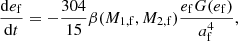
In general, this relation indicates that a typical GC witnesses, on average, 900 interactions in 12 Gyr. Figure 1 shows this correlation for the MOCCA models containing a BH subsystem (Arca Sedda et al. 2018; Askar et al. 2018), highlighting that the denser the cluster and the BH subsystem, the larger the number of BHB–BHB interactions. We note that the number of scatterings seems to depend on BHS mass, that is, on the number of BHs retained in the host cluster. In particular, we see that, at a fixed value of ρ12, a heavier BHS favours a larger number of scattering.
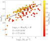 |
Fig. 1. Total number of BHB–BHB interactions as a function of the central density of the host GC at 12 Gyr in the MOCCA database. Colour coding shows the mass of the BH subsystem in the host globular cluster core. |
We explore the MOCCA database to determine the properties of the binary scatterings in terms of dynamical parameters, namely the semi-major axes and eccentricities of the two binaries, the masses of the BHs involved, the position of the binaries during the scattering, and the velocity dispersion of the cluster at the time of the scattering. We find that all scatterings are hyperbolic, and 97% of them take place in environments with a velocity dispersion in the range σc = [1 − 20] km s−1, with more than 81% being characterised by σc = [5 − 15] km s−1. Around ≳79% of the scatterings take place in a regime of strong deflection, meaning that the angle δ between the inward and outward directions of the centres of mass of the two binaries exceeds 90°, and involve BHs with masses larger than MBH > 10 M⊙. These interactions are the most energetic and have the largest probability of causing substantial evolution in one or both binaries and can, in some cases, trigger the formation of a triple (Bacon et al. 1996; Fregeau et al. 2004; Zevin et al. 2019).
In order to assess how frequently a triple might form from a binary–binary scattering, we create a sample of 500 binary–binary scatterings with properties extracted directly from binary–binary interactions occurred in MOCCA models, namely the binary component masses, semi-major axis, and eccentricity. We name this simulation set MOCC.
Our main purpose is to demonstrate that binary–binary interactions can form a significant number of triples, a fraction of which will be in a non-hierarchical configuration. A detailed study of the outcomes of binary–binary interactions in MOCCA models and their implications for BH mergers is left to a follow-up work.
It is important to stress that the MOCCA database contains models spanning a wide range of initial conditions, like the cluster initial mass and metallicity, the fraction of primordial binaries, the stellar prescription adopted, the location in the Galaxy, and the initial concentration and depth of the potential well. Such a heterogeneous mixture of variables can impact the properties of binary–binary scatterings in a non-trivial way, possibly leading to biased configuration parameters. Therefore, we carry out three additional simulation sets, modelling binary–binary hyperbolic encounters with well-defined properties for comparison with MOCCA models. For these models, we assign binary velocities assuming that the velocity dispersion at the time of the scattering is either σc = 5, 10, or 15 km s−1, thus bracketing the values that characterise MOCCA models, performing 500 simulations for each value. In the following, we refer to these additional models as BIN0, BIN1, and BIN2 (see Table 1).
Main properties of four-body models.
Whilst for MOCC simulations we extract all the parameters of the hyperbolic trajectories from MOCCA modes, to initialise the binary scattering in sets BIN0-1-2 we define the interaction semi-major axis

where μ = G∑imi is the gravitational parameter and v∞ = v12 − v34 is the relative velocity between the binaries. The velocities of the two binaries are then drawn from a Maxwellian distribution characterised by dispersion σc and used to calculate v∞. A hyperbolic encounter can also be characterised through two further parameters, namely the impact parameter and the deflection angle. The former is defined as  , while the latter represents the angle δ between the inward and outward direction of the motion of binaries centres of mass and is connected to the eccentricity parameter via equation
We note that the limit of large deflection angles, δ > π/2, corresponds to the strong deflection regime.
We draw the initial impact parameter assuming that it follows a linear distribution, as expected from simple geometrical arguments, for an isotropic velocity distribution f(b)db ∝ 2πbdb. We limit the distribution between a minimum bmin = 0, corresponding to head-on trajectories, and bmax, which is set in such a way that the maximum pericentre passage rp, 4b, max is limited to five times the largest semi-major axis of the two binaries, where  .
.
Binary component masses are extracted between 10 M⊙ and 50 M⊙, assuming a mass function f(m)∝m−2. Binary semi-major axes are drawn between 0.1 and 10 times the hard binary critical value (Heggie 1975), which is  according to a flat distribution in logarithmic values, whereas their eccentricities are selected from a thermal distribution (Jeans 1919). All other orbital parameters for each binary –longitude of periastron and ascending node, and mean anomaly– are selected randomly between 0 and 2π.
We note that the initial conditions adopted for model sets BIN0, BIN1, and BIN2 are in broad agreement with the binary–binary scattering properties extracted directly from MOCCA models.
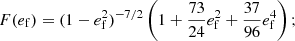
All binary–binary simulations are halted if one of the four BHs is ejected away or if the BHBs reach a final distance comparable to the initial one, that is, the two BHBs are completely unbound. The evolution of one typical example is shown in Fig. 2.
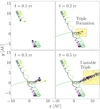 |
Fig. 2. Binary–binary interaction in one of the cases investigated. After the close encounter, one BH is ejected and the remaining three BHs form an unstable triple. |
3.1. Properties of triples formed from binary–binary scatterings
The main end states of a binary–binary scattering can be either one or two bound BHBs, or a bound triple. In the latter case, we usually distinguish between an inner binary, i.e. the most bound BH pair, and an outer binary composed of the inner binary centre of mass and the third bound object.
Whenever a BHB is left behind the binary scattering, it will undergo coalescence due to angular momentum loss via GW emission over a timescale (Peters 1964)
where
provided that either the BHB has no further companion or the perturbation of the third BH on the evolution of the inner binary is negligible.
In the following, we focus mainly on the properties of triples. For clarity, we summarise the nomenclature used to identify the orbital parameters of the inner and outer orbits:
-
a is semi-major axis;
-
e is eccentricity;
-
R = a(1 − e) is the binary pericentre;
-
ω is the argument of pericentre;
-
Ω is the longitude of the ascending node;
-
ϖ = ω + Ω is the longitude of pericentre;
-
tGW is the GW timescale;
-
i is orbital inclination.
The subscript ‘3’ is used to label the quantities related to the outer binary. The inclination is the angle between the angular momentum vectors of the inner and outer binaries.
Figure 3 shows the distribution of semi-major axis and eccentricity for the inner and outer binaries of triples formed from BHB–BHB scatterings. The figure highlights how an increase in the velocity dispersion generally corresponds to a decrease in the semi-major axis of both the inner and outer binary. In particular, the inner and outer binaries are in the range (5 − 3000) AU. Also, the overlap between inner and outer binary semi-major axis values implies the potential formation of triples whose evolution is chaotic. It is worth noting that triples formed in this way are equally distributed between prograde (inclination cos(i) > 0) and retrograde (cos(i) < 0) configurations, as shown in Fig. 4. As we discuss in the following sections, the relative orbital direction plays a critical role in determining the fate of the inner binary.
 |
Fig. 3. Top figure: distribution of semi-major axis for the resulting outer (filled blue steps) and inner binaries (filled green steps) following the binary–binary scatterings. Bottom figure: eccentricity distribution of the outer and inner binary, using the same colour-coding as in the top figure. In both figures, panels from top to bottom refer to cluster velocity dispersion values σc = 5 − 10 − 15 km s−1, respectively. |
A triple system is stable if the semi-major axis of the inner binary remains secularly constant, while for unstable systems the chaotic nature of the system leads to energy transfer between the components. Mardling & Aarseth (2001) determined a stability criterion through Newtonian N-body simulations, defined as (see also Antonini et al. 2014; Toonen et al. 2016)

where a (a3) is the inner (outer) orbit semi-major axis, and
![$$ \begin{aligned} K_{\rm stab} = \frac{3.3}{1-e_3}\left[\frac{2}{3}\left(1+\frac{M_3}{M_{\rm BHB}}\right)\frac{1+e_3}{(1-e_3)^{1/2}}\right]^{2/5}\left(1-0.3 \frac{i}{\pi }\right), \end{aligned} $$](/articles/aa/full_html/2021/06/aa38795-20/aa38795-20-eq10.gif)
which implies, in general, that larger inclinations reduce the critical value. We note that for a co-planar, prograde, and circular outer orbit and an equal-mass triple, M3 = 0.5 MBHB, the stability criterion implies K ≃ 0.3, and reduces to K ≃ 0.19 for retrograde motion with e3 = 0.5. Depending on the orbital configuration, after formation the triple can develop KL cycles (Lidov 1962; Kozai 1962) according to which the inner binary eccentricity can undergo a periodic oscillation depending on the mutual inclination. In a multiple expansion of the triple Hamiltonian, the leading order KL cycles are caused by the quadrupole term. In this case, KL oscillations can develop over a timescale of
where P1(3) is the orbital period of the inner(outer) binary, and drives the inner binary to reach a maximum eccentricity of
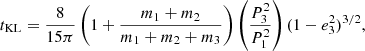
We note that the onset of KL oscillations can drive the system away from stability, especially in the case of highly inclined and retrograde orbits (see e.g. Grishin et al. 2017). In cases where the octuple term is non-negligible, the secular perturbation from the outer BH can drive the inner binary eccentricity to values close to unity. This is called the eccentric Kozai-Lidov (EKL) effect (Blaes et al. 2002; Naoz et al. 2011, 2013a; Lithwick & Naoz 2011; Katz et al. 2011; Naoz 2016). A general criterion to identify potential configurations that can be prone to the KL mechanisms is (for a review, see Toonen et al. 2016; Naoz 2016)
Figure 5 shows the values of Kstab and ϵKL normalised to their critical values for all triples formed in set BIN2. We find that around 18% of models do not fulfill either of the two criteria, thus implying that their evolution can be substantially driven by instabilities and/or chaotic processes.
 |
Fig. 5. Surface number density for the stability and octupole-level approximation criteria for triples formed in model BIN2. The two dotted lines delimit regions where the effect of octupole level approximation can become important (left side of the vertical line) or the triple is stable according to the Mardling & Aarseth (2001) criterion (upper side of the horizontal line). |
As these triples or the binaries left after the binary–binary interaction will be embedded in the host cluster, their disruption will take place over an evaporation time (Binney & Tremaine 2008):
where  is the average density of a star cluster with mass MGC and half-mass radius Rh, lnΛ = 6.5 is the Coloumb logarithm, m* = 1 M⊙ is the average stellar mass, and msys is the mass of the system considered, that is, either a triple or a binary. To calculate this quantity for our models we adopt a half-mass radius of Rh = 3.2 pc, i.e. the average value of observed GCs, and use the relation between σc, MGC, and Rh described in Arca Sedda (2020) to calculate the cluster mass. In the following we identify the evaporation time for triples with pedix evap, 3 and that for binaries with evap, 2.
At the end of each simulation we check whether (i) at least one binary hardened as a consequence of the scattering, or (ii) a bound triple was left behind following the interaction, and we derive the orbital parameters of any triple, short- or long-lived, formed during the binary scattering evolution. We note that the formation of a short-lived triple can fall in case (i), as these systems tend to eject one of the components and leave a tight binary as final state.
Figure 2 represents one such case: a triple clearly forms as a consequence of the BHB–BHB scattering but eventually breaks up, and therefore its end state is composed of two single BHs and a bound BHB. We note that it is possible for the same BHB–BHB system to develop a temporary triple more than once, and therefore the total number of triples can exceed the number of simulations run.
In case (ii) on the other hand, we distinguish three classes of triples depending on their orbital properties:
– hierarchical triples: bound triples with a3(1 − e3)/a > 10 [fhie];
– unstable triples: bound triples for which Eq. (6) is not satisfied [funs];
– octupole triples: bound triples that could undergo secular effects like KL cycles, which have ϵKL < 0.1 [foct] (see Eq. (10)).
We note that these conditions are not mutually exclusive, as one system can undergo several of the phases above during its evolution. Here, we define a triple whenever three of the four BHs are gravitationally bound; thus we include short-lived systems. According to the classification above, in sets BIN0-BIN1-BIN2 we find that almost half (fhie ∼ 43 − 53%) of the temporary triples have a3(1 − e3)/a > 10 and are thus, potentially, hierarchical. Around foct = 68% of triples have the octupole parameter ϵ < 0.1 and satisfy the Mardling & Aarseth (2001) stability criterion. Around funs = 34 − 39% of models do not fulfill the Mardling & Aarseth (2001) criterion. Finally, a significant fraction (fstab + oct = 25 − 33%) of triples satisfy both the stability criterion and have the octupole parameter ϵ < 0.1.
The binary–binary scatterings tailored to MOCCA initial conditions (set MOCC) return similar results, where around 58% of the triples are in a hierarchical configuration and ∼30% are in an unstable configuration. The vast majority of the temporary triples break up and recombine into triples multiple times, suggesting that this type of triple could play a major role in dense clusters, where BHB–BHB interactions are frequent. In some cases, the perturbations induced by the outer BH or by one BHB can trigger the swift coalescence of the other BHB, provided that the timescales involved are compatible with the evaporation time of the system.
If the binary scattering leaves behind a stable triple, and the KL timescale is shorter than the triple evaporation time, then KL oscillations can develop before the triple is ionised by a further stellar encounter. This mechanism drives the inner binary eccentricity up to emax and causes a periodic burst of GWs that shortens the binary lifetime. Under such circumstances, the inner binary undergoes a merger over a timescale of (Wen 2003; Antonini & Perets 2012)
where a and e represent the semi-major axis and eccentricity of the inner binary at the triple formation.
Two interesting examples of the evolutionary history of merging BHBs are displayed in Fig. 6. In the first, taken from set BIN1, the binary scattering drives the formation of a hierarchical triple with an inner binary (M1 + M2) = (23 + 18.4) M⊙ of semi-major axis a = 2.4 AU and eccentricity e = 0.8, and an outer binary with (M3, a3, e3) = (35.5 M⊙, 26.2 AU, 0.52). The inner binary undergoes several KL oscillations that drive the eccentricity up to emax = 0.99995, as shown in Fig. 6, leading ultimately to the inner binary merger over a total timescale of 103 yr, with about ∼530 yr spent in the hierarchical configuration. We note that the merger time calculated with Eq. (12) adopting the same emax value returns a merger time of 616 yr, thus fully compatible with the full N-body model.
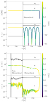 |
Fig. 6. Top panel: time evolution of the inner binary eccentricity in the simulated triple BIN1-374. At ∼460 yr, the binary–binary scattering drives the formation of a triple arranged in a hierarchical configuration, while the fourth object is ejected away. KL oscillations are apparent after the formation of the triple system. Bottom panel: same as above, but for model BIN2-152. In this case, the rapid variations are due to the chaotic interaction with the outer perturber, itself attributable to the formation of a non-hierarchical triple. In both cases, colour-coding marks the mutual inclination. |
In the second example, taken from set BIN2, the scattering drives the formation of a non-hierarchical triple that eventually forms a hierarchical triple and triggers the inner BHB merger on a short timescale of ∼102 yr. In this case, the inner binary is characterised by BH masses (M1 + M2) = (11.6 + 10.4) M⊙, semi-major axis a = 0.66 AU, and eccentricity e = 0.78, while the outer orbit is characterised by (M3, a3, e3) = (13.9 M⊙, 8.75 AU, 0.72).
More generally, we can distinguish several pathways to BHB mergers depending on whether or not the binary scattering:
1. Leaves behind a BHB with a final merging time smaller than 14 Gyr and an evaporation time of tGW < min(14 Gyr, tevap);
2. Induces the formation of a stable triple characterised by an inner binary with a merging time of tGW < min(14 Gyr, tevap, 2) and a KL time longer than the triple evaporation time (tKL > tevap, 3). In such a case, stellar interactions are likely to ionise the triple before KL oscillations take place;
3. Induces the formation of a stable triple with tKL < tevap, 3. In this case, KL oscillations develop before the triple evaporates and can drive the inner BHB to merger;
4. Induces the formation of an unstable triple for which the inner BHB merger time is shorter than the triple evaporation time (tGW < tevap, 3) and tGW < min(14 Gyr, tevap, 2); thus the binary likely merges before the triple is ionised;
5. Induces the formation of an unstable triple with tGW > tevap, 3 and tGW < min(14 Gyr, tevap, 2); thus the triple is ionised before the inner BHBs merge.
According to the merger classes defined above, we find that BHB–BHB scattering leads to at least one bound BHB with a merger time shorter than the evaporation time for 69 − 84% of the cases, while the end state is a bound triple for around 20.4 − 31.2% of the cases.
In the following section, we model the evolution of triples with properties extracted from the binary scattering model set BIN2, i.e. the one with the greatest chance of producing unstable triples, which are the main focus of this work.
3.2. Evolution of back hole triples in astrophysical systems: implications for binary mergers
In this section we model the evolution of triples whose initial conditions are drawn from the results of our BHB–BHB scattering experiments described in Sect. 3. On the one hand, this enables us to focus only on the formation of triples, rather than on the much larger parameter space that characterises binary–binary scatterings, whilst on the other, it permits us to obtain the general properties of potential BHB mergers originating from this channel, and to compare them with present-day GW detections. We ran 1000 simulations drawing the initial inner and outer semi-major axes, eccentricity, and mutual inclination from the distribution obtained for the BIN2 simulations set, which assumes a host cluster with velocity dispersion σ = 15 km s−1 (see Figs. 3 and 4).
In the following, we refer to these triple models as SET0, as summarised in Table 2. The main objective of these simulations is to determine the role played by both hierarchical and non-hierarchical triple evolution in the formation of BHB mergers.
Main parameters of the numerical models.
To identify potential mergers we calculate the merger time in two different ways, depending on the level of hierarchy of the triple as discussed in the previous section. For each triple, we calculate the Mardling & Aarseth (2001) stability criterion, a3, f/af < K (see Eq. (6)), and the octupole-level approximation criterion ϵoct < 0.1 (see Eq. (10)). In the case in which the triple does not fulfill these criteria or is disrupted, we calculate the merger time using Eq. (4). If, instead, the triple satisfies both criteria above, the merger time is calculated following Eq. (12).
As summarised in Table 3, we identify 218 mergers out of 961 models in this way, corresponding to a merger probability of 22.7%. At the end of the simulation, around ∼92.5% of the merger candidates are the inner BHB in a triple that satisfies both stability and octupole criteria (a3, f/af < K; ϵoct > 0.01); we therefore classify these as hierarchical mergers, whereas the remaining 7.5% are BHBs originating from disrupted triples. It must be noted that around two-thirds of the triples are initially in a hierarchical configuration because of the constraints imposed by the binary scatterings, which partly explains the much larger number of hierarchical mergers compared to non-hierarchical ones.
Mergers in SET0.
We also find a subclass of systems characterised by a peculiar behaviour in the evolution of the eccentricity, which differ substantially from the standard KL predictions. Figure 7 shows three systems in this sample, one showing typical KL eccentricity variation, one showing the peculiar KL-like cycles mentioned above, and the latter showing the case of a disrupted triple.
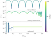 |
Fig. 7. Eccentricity variation as a function of time in three systems that lead the inner binary to merge. Top panel: triple in which the inner binary undergoes typical KL oscillations. Central panel: case where KL oscillations vary in phase and amplitude over time. Bottom panel: case of a disrupted triple, with the inner binary evolution driven solely by GW emission. |
The top panel of Fig. 8 shows the distribution of initial and final values of the inclination for all BHBs in SET0. We find that the interaction with the perturber tends to decrease the fraction of retrograde systems: the initial models are equally distributed between prograde and retrograde configuration, whereas, at the end, prograde configurations outnumber retrograde ones by a factor of 1.34. This suggests that retrograde systems have the tendency to reduce the inclination, and flip the orbit in some cases, whereas prograde systems tend to maintain their original configuration. Limiting the analysis to mergers, we find that the population concentrates around nearly perpendicular configurations, that is, with cos(i)≃0, as shown in Fig. 4.
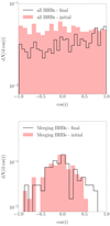 |
Fig. 8. Top panel: initial (red filled boxes) and final (black open steps) inclination distribution for all BHBs in SET0. Bottom panel: same as above, but only for merging BHBs in SET0. |
As shown in Fig. 9, the mass distribution of the primary in merging BHBs of SET0 appears to be almost flat, with a weak peak at values M1 = 15 − 25 M⊙. The mass distribution of the secondary component on the other hand shows a strong peak at values M2 = 10 M⊙ and a sharp decline at values M2 > 20 M⊙. As a result, 50% of the mergers in SET0 have a mass ratio in the range q = 0.2 − 0.6.
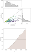 |
Fig. 9. Top panel: combined mass distribution of merging BHB components for SET0. The dashed line identifies loci in the plane at a fixed value of the mass ratio. Darker(lighter) colours identify larger(smaller) mass ratios. Bottom panel: mass ratio distribution for merging BHBs in SET0. |
Around 18% of models undergo a component swap. Among them, in a few cases (3%) the outer BH mass initially exceeds the whole BHB mass, MBHB < M3, and therefore the component swap determines the formation of a final BHB that is much heavier than the initial one. The majority of component swaps (15.2%) lead to a final BHB in which the companion is heavier than the original, which confirms that component exchanges tend to promote an increase in the binary binding energy. However, component exchanges affect only 4.6% of all mergers (10 mergers out of 216). In eight of these cases, the BHB mass changes by less than 20% whereas in the remaining two cases the new companion increases the BHB mass by a factor of 1.3 and 1.8, respectively, acquiring a net positive gain of 10 M⊙ and 30 M⊙ respectively.
In Sect. 4, we explore the role of the triple configuration in determining the formation of merging BHBs.
3.3. Gravitational wave emission frequency and merging BHB eccentricity
The GW signal emitted during BHB evolution is characterised by a broad frequency spectrum, whose peak frequency can be calculated as (Wen 2003; Antonini et al. 2014)
As noted by Antonini et al. (2014), the maximum eccentricity attainable by the inner binary can be expressed as
![$$ \begin{aligned} \sqrt{1-e_{\rm max}} = 5\pi \frac{M_{\rm 2,f}}{M_{\mathrm{BHB},\mathrm{f}}}\left[\frac{a_{\rm f}}{a_{\rm 3,f}(1-e_{\rm 3,f})}\right]^3\cdot \end{aligned} $$](/articles/aa/full_html/2021/06/aa38795-20/aa38795-20-eq18.gif)
The equation above can be used to constrain the region of parameter space in which the BHB can attain an eccentricity above 0.1 at frequencies audible to a ground-based detector, a condition that can be expressed as 3 < a3, f(1 − e3, f)/a1, f ≲ 10 in the case of BHBs with components of comparable mass. It must be noted that our models are wider systems compared to those used by Antonini et al. (2014). As shown in the following, this significantly reduces the probability of observing eccentric binaries in the Hz band.
In ARGdf, the last phases before the binary merger are extremely time consuming because the code needs extremely small steps to precisely integrate the equation of motion of the components. In order to find a good balance between computational load and modelling reliability, for each binary we numerically integrated the Peters (1964) equations:
with

These equations have analytical solutions for af(ef) (Peters 1964) and time evolution (Mikóczi et al. 2012). For each simulation, we select the (af, ef, MBHB, f) values available at the last snapshot and we use them to integrate the equation above. This choice implies three possibilities: (a) if the triple breaks up before the simulation ends, the values at the last snapshot represent the BHB end state, (b) if the inner BHB merges before the simulation ends, the values at the last snapshot represent the BHB status if the outer BH does not have any effect on the inner BHB evolution, or (c) if the triple is still bound but the inner BHB merger time is smaller than 14 Gyr, we take the maximum eccentricity if the binary is classified as hierarchical or the value at the last snapshot otherwise. Figure 10 shows the cumulative distribution of the eccentricity of merging BHBs calculated in different frequency windows, namely f = 10−3, 10−2, 10−1, 1, 10 Hz.
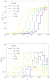 |
Fig. 10. Cumulative distribution eccentricity (top panel) and its distribution (bottom panel) for all the BHB mergers in model 11. The eccentricity is calculated as the BHB crosses a given frequency, as indicated in the legend. The dotted line indicates a value of eccentricity of e = 0.1. |
We find that around 60% of mergers have a noticeable eccentricity e > 0.1 in the LISA frequency band (Amaro-Seoane et al. 2017), i.e. f = [10−4 − 10−2] Hz, whereas this fraction drops to 3% for eccentric mergers falling in the LIGO-Virgo-sensitive band, f > 1 Hz.
Interestingly, around one-third of the mergers that are eccentric in the LISA band form from non-hierarchical triples. More specifically, ≳75% of non-hierarchical mergers are potential eccentric LISA sources, while this percentage decreases to 60% for hierarchical mergers. This suggests that the chaotic evolution of non-hierarchical triples might cause them to form eccentric sources with greater efficiency, at least at low frequencies and for environments typical of GCs.
4. Numerical simulations of non-hierarchical triples
In the previous section, we show that non-hierarchical triples can constitute around two-thirds of triples formed in binary scatterings in dense clusters. Our results suggest that mergers from non-hierarchical triples can constitute around 10% of all mergers from triples and that around 80% of them will show significant eccentricity in the LISA band. Moreover, our preliminary analysis discussed in the previous section suggests that the configuration of the triple might play a role in determining the final fate of the inner BHB. In the following, we therefore focus on the evolution of non-hierarchical and mildly hierarchical triples to assess the importance of the orbital configuration in determining the fate of the triple.
In an attempt to discern what parameters are most effective in determining the states emerging from the triple evolution, in the following we present and discuss 30 000 simulations gathered in ten groups, performed using ARGdf (Arca-Sedda & Capuzzo-Dolcetta 2019). The main features and initial values for each set are summarised in Table 2. As in the case of co-planar orbits the argument of node Ω is ill-defined, in the table we refer to Δϖ as the difference between the inner and outer binary longitude of pericentre. In non-coplanar cases, this quantity reduces to Δϖ=ω, as we fixed all the other terms initially to zero.
As opposed to simulation SET0 (discussed in Sect. 3), which includes initial conditions drawn from BHB–BHB scattering, in this section we study a large series of non-hierarchical triple simulations (SET1-10) characterised by an inner binary with predefined properties. These sets of simulations allow us to carry out a systematic analysis of how the evolutionary outcome depends on the initial conditions for non-hierarchical triples. Simulation sets from SET1 to SET4 are designed to explore the role played by the inner binary eccentricity and the outer binary inclination, SET5 to SET8 allow us to quantify the dependence on the orbital orientation, and SET9 and SET10 are devoted to investigating the role of the mass of the tertiary component and, more generally, the distribution of the outcome of the triple evolution if changing all the orbital parameters. As shown by Table 5, in all the cases but SET9 and SET10, we set the inner binary pericentre to Ri = 20 AU and masses (20 M⊙, 10 M⊙, 20 M⊙) implying tGW, i = 1018 Gyr for a circular binary. In SET10, instead, we choose Ri = 1 AU, a value typical of binaries forming in the densest regions of globular and nuclear star clusters (Heggie 1975; Miller & Lauburg 2009; Antonini et al. 2016) for which tGW, i ≃ 3000 Gyr for ei = 0.
We stop our simulations if one of three conditions is satisfied: (1) the triple breaks, (2) two components merge, or (3) the integration time exceeds 5 Myr. The latter condition allows us to identify stable or meta-stable triples on this timescale. The initial value of the inner binary orbital period is in between ∼1 and 100 yr in all the sets.
4.1. Dynamics of bound triples: an interesting reference case
The behaviour of an unstable bound triple cannot be described through a secular approximation formalism, as the triple lifetime is usually comparable to a few orbital periods of the outer binary (see Fig. 3). We look for the distinct statistical features in the evolution of these systems using direct three-body simulations. For the sake of simplicity, in the following the subscript f(i) denotes final(initial) quantities. First, let us assume the case of a BHB comprised of BHs with masses M1, f = 20 M⊙ and M2, f = 10 M⊙, characterised by an initial eccentricity ei = 0 and semi-major axis ai = 20 AU. The BHB is orbited by a third BH, with mass M3, i = M1, i, initially placed at a pericentral distance R3, i = 200 AU from the inner binary centre of mass, with eccentricity e3, i = 0.7. In the following, we refer to the BHB as the inner binary and to the system composed of the centre of mass of the inner binary and the third BH as the outerbinary.
Figure 11 shows how the two systems evolve in time. In the case of an initial prograde configuration (top panel in Fig. 11), the triple breaks immediately after the first passage at pericentre (∼100 yr), and the outer BH swaps with the lighter component of the initial inner BHB. The lighter BH is ejected and the new BHB is composed of two equal-mass BHs with eccentricity ei ≃ 0.15 and semi-major axis ai = 24.3 AU.
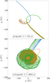 |
Fig. 11. BHB–BH trajectory for a non-hierarchical triple initially in a prograde (top panel) or retrograde (bottom panel) configuration. The time indicated in the figure marks the moment at which the triple breaks up. |
In the case of an initially retrograde configuration, instead, the overall picture is much more complex. The inner and outer binary orbits undergo mutual precession for 21 orbital periods of the outer binary. During this phase, the eccentricities and semi-major axes develop several oscillations, as shown in Fig. 12, which culminate after ∼6 × 10³ yr in a series of strong and repeated scatterings. During this phase, which lasts for ≳600 yr, the inner binary changes its components frequently until the triple breaks up. The lighter object is again ejected and the resulting binary is now composed of two equal-mass objects, each of 20 M⊙, a separation slightly larger than its initial value, af = 25 AU, and a high eccentricity ef = 0.999275. The corresponding coalescence timescale for such a system is tGW, f ≃ 1.68 Gyr, thus suggesting that counter-rotation can facilitate coalescence in non-hierarchical triples.
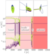 |
Fig. 12. From top to bottom: semi-major axis and eccentricity of the inner (red solid line) and outer binary (black dotted line) for the triple shown in the bottom panel of Fig. 11. The system shows a bound triple in the first ∼4000 yr, then one object marked with light blue is ejected on a weakly bound eccentric orbit, and is ultimately completely ejected on an unbound trajectory. |
The overall evolution of the initially counter-rotating triple, sketched in Fig. 12, can be divided into four main stages. In stage I, the inner and outer binary orbits undergo precession, the outer semi-major axis a3 slowly decreases while a increases. Moreover, the outer binary decreases its average eccentricity, while the inner binary eccentricity increases up to 0.6. At some point (stage II) the three objects come close enough that the triple loses any kind of hierarchy. A short phase of scatterings drive the formation of a binary composed of the outer BH and the heavier component of the inner binary (red and blue lines in Fig. 12) while the original secondary of the inner binary is pushed toward a wider, nearly parabolic but bound orbit. The next close approach of the third object leads to a new series of strong interactions (stage III), which results in the ultimate disruption of the triple. This complex series of interactions leaves behind a highly eccentric binary composed of the two most massive members of the triple (stage IV).
The evolutionary differences between the initially prograde and retrograde cases could be related to the different levels of stability in the two configurations, as made evident in the Mardling & Aarseth (2001) stability criterion. In our reference model, a3/a ≃ 5.9, while the critical value for stability (see Eq. (6) above) is K = 12.7 for a retrograde configuration and K = 18 for a prograde configuration, thus a3/a < K in both cases. The triple is initially unstable and the evolution is chaotic (see Grishin et al. 2017, 2018, for results in the non-coplanar case).
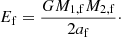
The simple model presented above shows, at a glance, the importance of the triple orbital configuration, which can lead to enormous differences in the final status of the system. Some of these results may be explained by energy and angular momentum transfer during the repeated close interactions. The initial total energy of the system is given by the sum of the binding energies of the inner and outer binary, namely
where Hint is the interaction energy term, which is usually small in the hierarchical limit (Harrington 1968). Assuming that the binary breaks up after several interactions, ultimately producing a binary and an unbound star, and that the energy taken away is much larger than the interaction energy, the final energy budget will be dominated by the binary binding energy
The difference between the final and initial energy must equal the kinetic energy of the escaping third object and the centre of mass of the final binary, which is non-negative (Ef − E0)≥0. Combining and re-arranging the equations above yields a constraint on the final binary hardness
![$$ \begin{aligned} \frac{M_{\rm 1,f}M_{\rm 2,f}}{a_{\rm f}} \ge \left[1+\left(\frac{M_{\rm 3,i}}{M_{\rm 1,i}}+\frac{M_{\rm 3,i}}{M_{\rm 2,i}}\right) \frac{a_{\rm i}}{a_{\rm 3,i}}\right]\frac{M_{\rm 1,i}M_{\rm 2,i}}{a_{\rm i}} > \frac{M_{\rm 1,i}M_{\rm 2,i}}{a_{\rm i}}\cdot \end{aligned} $$](/articles/aa/full_html/2021/06/aa38795-20/aa38795-20-eq26.gif)
Thus, the disruption of the triple inevitably leads to the formation of a harder binary, either by shrinking (af < ai) or acquiring a heavier component (M2, f > M2, i) via component swap. In the representative example presented above, the final binary mass increases by a factor 3/2 due to the swap of the outer BH and the secondary component of the inner binary, while its semi-major axis remains almost constant. Let us now consider the triple angular momentum L = LBHB + L3. In the simplest approximation that the triple is initially coplanar, the norm of the angular momentum vector is simply Li = LBHB, i ± L3, i, where the sign +(−) identifies an initially prograde(retrograde) configuration. When considering the case in which the triple flips configuration, given the angular momentum conservation, we can write the final BHB angular momentum as
where the two equations hold for a flip from a prograde to a retrograde configuration and vice versa. The two equations above tell us that in a prograde-to-retrograde flip the BHB acquires angular momentum (LBHB, f > LBHB, i), implying that its eccentricity decreases, whereas for the opposite flip, LBHB, f < LBHB, i, and the final eccentricity increases. Therefore, from energy and angular momentum conservation we find that
– the final binary is harder, either by becoming tighter or more massive, than the initial inner binary;
– orbital flips can determine the increase (from retrograde to prograde orbits) or decrease (from prograde to retrograde orbits) of the BHB eccentricity.
In the example presented above, we note that the initial merger time for the inner BHB is tGW, i = 8.7 × 10¹⁸ yr, which is much larger than a Hubble time. However, as a consequence of the triple evolution, the GW timescale of the resulting BHB reduces in both the configurations because of the efficient energy transfer that drives the component swap. In the prograde case, the final BHB GW time is still larger than a Hubble time, but in the retrograde configuration the GW timescale drops by nine orders of magnitude, to tGW, f = 1.68 Gyr. Hence, this process facilitates the formation of merging binaries. In the following section, we explore in detail how GW times change in non-hierarchical and unstable triples, and which orbital configurations favour a more efficient shrinkage of the inner BHB.
4.2. Distribution of GW merger times
As a first step, we exploit SET4 and SET10 to explore how the evolution of a non-hierarchical triple affects the BHB merger time. In these simulation sets (see Table 2) (a) the initial pericentre is fixed at 20 AU and 1 AU, respectively; (b) the initial eccentricity and inclination are widely distributed; and (c) the BH masses are either fixed or allowed to vary, respectively. Figure 13 compares the initial and final distribution of the merger times for all the models in SET4 and SET10. The broadening of the merger-time distribution is apparent in both cases, falling below 14 Gyr in five cases in SET4 (0.25% of the total sample) and in up to 677 cases in SET10 (8.5%).
 |
Fig. 13. Initial (filled red boxes) and final (blue steps) GW merger time distribution for all BHBs in SET4 (top panel) and SET10 (bottom panel) (see Table 2 for parameters). The dotted vertical line marks tGW = 14 Gyr. A broad tail extending to low GW timescales is produced with |

The results show that the GW merger-time distribution approximately follows a power law of
or equivalently
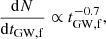
for both SET4 and SET10 for GW timescales of less than its initial value. This outcome is mostly due to the fact that tGW, f given by Eq. (4) is most sensitive to the eccentricity, approximately as tGW, f ∝ (1 − ef)7/2. This implies that  , and so when all other parameters are fixed, we get
Thus, if 1 − ef is approximately uniformly distributed after the encounters, the distribution of the GW timescale follows  , that is
  . A similar argument shows that for fixed ef,
  . However, as shown in Fig. 14, we find that the final semi-major axis distribution spans typically only a decade around the initial semi-major axis distribution and many of the merging binaries have an eccentricity very close to 1 following the three-body dynamics. Thus the eccentricity distribution after the three-body dynamics is crucial for the GW merger-time distribution.
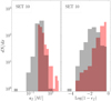 |
Fig. 14. Semi-major axis (left panel) and eccentricity (right panel) distribution for the initial inner BHB population (red filled boxes) and for mergers only (black steps) in SET10. |
4.3. Effects of initial eccentricity, inclination, and argument of pericentre
In this section, we focus on the role of the combined effects arising from the inner binary eccentricity and the outer binary inclination. The values allowed for the outer pericentre R3, i are, depending on the simulations set, between one and seven times the initial inner binary pericentre which typically represents a non-hierarchical system. Fixing the ratio between the initial pericentre of the inner and outer orbit and allowing the eccentricities to vary implies the possibility in some cases that Ri/(1 − ei) > R3/(1 − ei, 3), implying that the semi-major axis of what we identify as the inner BHB is actually larger than that of the outer one. Therefore, in the analysis presented below we remove all models that initially have Ri/(1 − ei) > R3/(1 − ei, 3), corresponding to around 10% of all models. Due to the assumptions made, the ratio a3, i/ai ranges between 1 and 103. We note that in set BIN2 (BHB–BHB scatterings) we find that 94% of triples have a semi-major axis ratio in the same range, and therefore this kind of configuration describes the majority of the triples formed in BHB–BHB strong encounters. The eccentricity is selected according to a thermal distribution (Jeans 1919) both for e3, i and ei, although in some sets the value of the inner BHB eccentricity is kept fixed, as listed in Table 2. We selected a co-planar, prograde configuration with ei = 0 as a reference model for SET1 simulations. In order to shed light on the importance of the orbital parameters, we then assumed 0 ≤ ii < 10° in SET2 and, along with this choice, we also vary ei in SET3. In SET4 we varied the outer inclination in the range 0 ≤ ii < 180°, thus investigating both prograde and retrograde orbits, and ei < 1, thus investigating the evolution of both circular and nearly radial BHBs. This sample of 5000 simulations gathered in four groups represents a quick way to highlight the differences between prograde and retrograde tight triple systems. These differences are further investigated in SET5 and SET6, where we examine exactly co-planar orbits in a co-rotating and counter-rotating configuration, respectively, with fixed inner binary eccentricity at ei = 0.6 and random Δϖi. SET7 and SET8 are nearly coplanar configurations where the eccentricity is drawn with 0 ≤ ii < 10° and 170 ° ≤ii < 180°, respectively, and, unlike in SET3, we set Δϖi = π.
The top four panels in Fig. 15 show the ratio between the final and initial value of the inner binary pericentre, rp, f/rp, i, plotted against the ratio of the initial apocentre of the outer binary to that of the inner binary, denoted R3, i/Ri, in the case of SET1 to SET4. The figure clearly shows that R3, i ≲ 5Ri is necessary for a significant decrease in the pericentre distance and the GW timescale for a nearly coplanar triple.
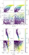 |
Fig. 15. Ratio between the initial and final values of the inner binary pericentre with respect to the outer binary initial separation, normalised to the inner BHB initial semi-major axis, ai = 20 AU. From left to right and from top to bottom panels: SET1 (ei = 0, Δϖi = 0 − 2π, ii = 0°), SET2 (ei = 0, Δϖi = 0, ii = 0 − 10°), SET3 (ei = 0 − 1, Δϖi = 0, ii = 0 − 10°), and SET4 (ei = 0 − 1, Δϖi = 0, ii = 0 − 180°), respectively; see Table 2. The colours represent the ratio between the final and initial value of the GW timescale for the inner binary. Bottom panels: same as in top four panels, but here we show the inner binary final eccentricity vs. the semi-major axis ratio. |
On the other hand, allowing both ii and ei to vary (SET3 and SET4) makes the distribution of ef and af much broader for all R3, i values. Indeed, in this case, even if the third BH initially moves relatively far from the inner binary, it can lead to a significant reduction of the inner binary pericentre and tGW, i. The bottom four panels of Fig. 15 show the final eccentricity of the inner binaries and the factor by which the semi-major axis changes. In SET1 and SET2 the semi-major axis is typically conserved to within a factor of two but the eccentricity is broadly distributed up to almost unity, also showing a correlation with af/ai. SET3 shows that when the inner binary initial eccentricity is allowed to vary then its semi-major axis can shrink by a larger factor and there is a larger fraction of highly eccentric sources. There is no prominent clustering or correlation in the case of SET4. We conclude that all orbital elements play a crucial role in determining the outcome of the triple evolution. Next we discuss the effect of the outer and inner eccentricity for nearly coplanar, prograde systems (SET1, SET2 and SET3) in more detail, and discuss the outer binary inclination in the following section.
4.4. The evolution of prograde and retrograde triples
In order to shed light on the evolution of triple systems, we calculated for SET4 the fraction of models that satisfy a particular constraint among all orbits that have an initial inclination smaller than a given value Δα and larger than π − Δα. In particular, we examine the fraction of simulations for which the merger time is decreased by a factor of 1, 0.1, or 0.01, as shown in Fig. 16. For instance, setting this fraction at Δα = 5° means that we consider only models for which ii < 5° (almost coplanar prograde) or ii > 175° (almost coplanar retrograde) and calculate the percentage of cases in which the merger time decreases by at least the given factor. We verified that, in both the prograde and retrograde subsamples selected at varying Δα, the number of objects is similar, and so the implications in the two cases have similar statistical significance.
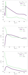 |
Fig. 16. Percentage of models with ii < Δα (red solid line) or ii > Δα (black dotted line) and tGW, f/tGW, i < 1, 0.1 and 0.01 (from top to bottom) in SET4. Nearly coplanar retrograde orbits have the highest probability of greatly reducing the GW timescale. |
In the top panel of Fig. 16 we show the fraction of binaries for which the GW timescale decreases as a function of Δα in the prograde and retrograde cases, respectively. The middle and bottom panels show cases where the GW timescale decreases by at least a factor of 10 or 100, respectively. We find that with the exception of nearly coplanar orbits Δα < 10°, prograde and retrograde orbits generate similar fractions at fixed δα to within ∼10%, with retrograde orbits producing slightly higher probability of decreasing the GW timescale by a factor of 100. The striking result of the figure is that the probability of decreasing the GW timescale by a factor of 100 is highly peaked at coplanar retrograde configurations.
More interestingly, the percentage of cases for which tGW, f/tGW, i < 100 is much higher for retrograde orbits, as shown in Table 4. This implies that retrograde configurations drive the formation of much tighter BHBs than prograde ones, and are therefore characterised by much shorter GW timescales.
Percentage of tightened BHBs.
After a few passages at pericentre, the triple can either break up or remain in a metastable or stable configuration, depending on the initial conditions. For instance, the triple disruption occurs in 93.3% of the models in SET4, highlighting the chaotic nature of such configurations. In the following, if the triple is disrupted and leaves behind a BHB and a BH, we calculate the inclination promptly after the disruption, thus measuring the angle between the angular momenta directions immediately after the BH ejection.
Under this assumption for disrupted models, we calculate the percentage of models that are in a prograde, ηpro, or retrograde, ηret, configuration by the end of the simulation.
This quantity allows us to quantify the occurrence of orbital flipping in our models. As long as the initial conditions assume an almost co-planar prograde configuration and zero eccentricity for the inner orbit (ii < 10°, SET1 and SET2) flipped systems are less than 0.02%. An eccentric inner binary (SET3) causes this percentage to slightly increase up to 3.4%. In the most reliable case in which the inclination is initially equally distributed among prograde and retrograde configurations (SET4) we find a clear excess of prograde systems (80.5%) compared to retrograde ones (19.5%). This likely implies that there is a preferential ‘direction’ toward which this kind of system evolves. We investigate this further in the following section.
This trend is outlined by Fig. 17, which shows a comparison between the initial and final distribution of the inclination cosine for all the models in SET4. Despite being almost flat initially, the distribution is evidently unbalanced after the triple evolution, which because the orbital flipping is more efficient for retrograde systems. At values cos(if) > − 0.8, the distribution seems well described by a power law. At smaller values, corresponding to inclinations if > 140°, the power law changes slope and maximises for co-planar retrograde systems.
 |
Fig. 17. Initial (filled red steps) and final (empty black steps) inclination distribution in SET4. |
4.5. The impact of coplanarity, inclination, e, and ϖ: orbital flipping and BHB merger
SET5 to SET8 are designed to help us better understand nearly coplanar systems and further constrain the differences between prograde and retrograde configurations.
In SET5 to SET8, the triple has a high probability of producing a binary and an unbound single. In coplanar prograde models (SET5), we find the maximum number of disruptions, Ndis = 1908, corresponding to ∼95.4% of the models investigated. Nearly coplanar retrograde models (SET7) have a somewhat smaller number of disrupted triples, Ndis = 1753, at around 87.7%. The BHB emerging from the triple break up has a final merger time that is at least ten times shorter than its initial value in over 45.7 − 67.2% of the cases, depending on the initial inclination, and maximises in the case of co-planar retrograde orbits with a mildly eccentric outer binary (SET6). A comparison between all these quantities, summarised in Table 5, suggests that the most effective configuration for producing merging BHBs is fully co-planar and retrograde.
Main results for SET4 to SET8.
Moreover, Table 5 shows the final number of models in prograde or retrograde configuration, respectively, for each simulation set, along with the percentage of those models that have a GW time ratio decreased to below 1 or 10−2 times its original value. In SET5, where we assumed an initially prograde configuration, we found that only 0.7% of models evolve toward a retrograde configuration. In all those cases, tGW decreases by a factor of 100 (fr0.01 = 100%), while among those that preserve the initial prograde configuration, the merger time decrease is less effective, being fp0.01 = 20.4%. On the other hand, when the initial configuration is retrograde (SET6), the triple tends to change configuration to prograde in two-thirds of the cases. We note that those triples that flip into a co-rotating configuration shrink as well, and therefore a reduction in the GW timescale, but the probability of the merger time decreasing by a factor of 100 is around fp0.01 ≲ 50%, while this probability is higher for simulations in which the initial counter-rotating property does not change, being fr0.01 ≃ 61%. Allowing small deviations from coplanarity and a distribution in the initial eccentricity does not change these results qualitatively. Of the initially prograde systems at low inclinations (SET7, i < 10°), only a handful of triples change to retrograde, with 96.9% of them achieving a factor of 100 reduction in tGW. For initially retrograde systems at inclinations above i > 170° (SET8), instead, 66% of the models flip but only 30% of them have tGW, f/tGW, i < 0.01. Therefore, as a general result we note that the criterion tGW, f/tGW, i < 0.01 is more common in retrograde cases that flip. From this comparison, we identify the following general properties of triple systems:
– triple systems tend to evolve toward co-rotation;
– the orbital flip causes, on average, the formation of a tighter inner binary system;
– nearly1 coplanar initially prograde and retrograde systems have a similar probability of decreasing the GW timescale by a factor of 100, but exactly coplanar retrograde systems are 2.5 times more likely to decrease the GW timescale by a factor of 100 than exactly coplanar prograde systems.
The final BHB components show clearly that inclination also affects the capacity of the outer BH to take the place of the lighter BHB components. Figure 18 shows the ratio of final-to-initial pericentre rp, f/rp, i as a function of the ratio between the initial values of the outer apocentre and inner pericentre, ra3, i/rp, i, for models that either preserve or exchange one of the inner BHB components in SET5 (prograde co-planar) and SET6 (retrograde co-planar). In initially prograde configurations, we see that swapped binaries tend to preserve their original orbits, showing rp, f/rp, i > 0.05 − 0.1, whereas for ‘original’ binaries this ratio can fall below 10−4 in a few cases, especially if ra3, i/rp, i < 100. For retrograde models, instead, the pericentre ratio is broadly distributed in the range 10−5 − 1 regardless of the component swap and the mass of the secondary companion, suggesting that in retrograde systems the exchange of a component does not impact the overall shrinkage of the binary.
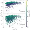 |
Fig. 18. Final inner binary pericentre as a function of the outer binary initial apocentre, both normalised to the initial pericentre of the inner binary for prograde (SET5, top panel) and retrograde (SET6, bottom panel) systems. Binaries maintaining their original components (10 M⊙ + 20 M⊙) are identified with blue dots, whereas those exchanging the lighter component are shown with green dots and identify final binaries with component masses 20 M⊙ + 20 M⊙. The final binary total mass is identified by the coloured map. |
5. Unravelling the host clusters of mergers with gravitational waves
As discussed in Sect. 3.2, BHB mergers developing in triples formed in clusters with σ = 5 − 15 km s−1 can appear as eccentric sources in the LISA and, less frequently, in the LIGO-Virgo observational window. We have seen that the properties of the merging BHBs from non-hierarchical triples depend on the triple configuration and orbital parameters. In this section, we exploit SET9 and SET10 to investigate whether or not it is possible to place constraints on the environment in which a BHB merger develops on the basis of the associated GW signal.
In SET9, where the triple configuration is similar to SET4 but the BH masses are allowed to vary, we find a merger probability of Pmer, SET9 = 0.25% (i.e. 15 mergers out of 8000 simulations), which is similar to SET4. This similarity is due to the fact that the GW time decreases most when the initial inner BHB mass is similar to that of the outer BH (MBHB, i/M3, i ∼ 1 − 3). Out of 15 mergers, we find 6 with an eccentricity above 0.1 when transiting in the mHz frequency window, and only 1 eccentric source in the 0.1 − 1 Hz range. In SET 10, instead, we find 677 merger events, corresponding to a Pmer, SET10 = 8.5%. This is clearly related to the choice of an initially tighter system. Among all the mergers, 273 occur in a prograde configuration, Pmer, pro = 6.8% of all the prograde models, while the remaining 404 come from retrograde configurations, Pmer, ret = 13.6%. This further confirms our earlier finding that, on average, models tend to evolve toward co-rotation, while the minority evolving from a co-rotation to a counter-rotation configuration shrink more efficiently and merge with a higher probability. As shown already in Fig. 13, the final GW time distribution exhibits two distinct features: a small peak corresponding to tGW, f = 104 yr, and an increasing trend in the time range 106 − 1010 yr, well described by a power law:  . Compared to the initial distribution, the final GW time distribution is much broader. Such broadening is caused by the tertiary BH perturbations, which increase the final eccentricity to values near unity.
All the models presented here have inner BHBs with a fixed initial pericentre of either 1 or 20 AU. However, dense stellar systems can contain much harder BHBs depending on the environment. A BHB is defined as ‘hard’ if its binding energy Eb exceeds the average field kinetic energy ⟨EK⟩, that is, if the semi-major axis is smaller than a limiting value ah:
As first described by Heggie (1975), hard binaries tend to become harder and harder as they interact with other stars, and are therefore the most likely to survive in star clusters. Figure 19 shows how Γh varies with the BHB semi-major axis assuming a BHB mass of either 10 (lower bound) or 30 M⊙ (upper bound). Monte Carlo models of globular clusters suggest that the population of BHBs that are processed via strong encounters and are ultimately ejected from the cluster have semi-major axes that are linked to the cluster mass and half-mass radius (Rodriguez et al. 2016),

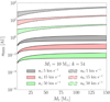 |
Fig. 19. Hard binary criterion Γh as a function of the BHB semi-major axis and for different values of the velocity dispersion of the host system, with the upper(lower) limit corresponding to a BHB mass of MBHB = 30(10) M⊙. The horizontal black line marks the boundary between hard and soft binary configurations. |
where k = 54 (Rodriguez et al. 2016), and μ12 = M1M2/(M1 + M2) is the BHB reduced mass. Following Arca Sedda (2020), we can connect the cluster mass and half-mass radius to its velocity dispersion via the relation
with α = 1.14 ± 0.03; we can therefore express the typical values of the semi-major axis of ejected BHBs in terms of the cluster velocity dispersion. Figure 19 shows how ah and ae vary assuming a primary BH with mass M1 = 10 M⊙ and cluster velocity dispersions of σ = 5, 15, and 50 km s−1. If we consider (ae, ah) as the limiting values of long-lived BHBs in dense clusters, we see that in dense nuclear clusters the tightest BHBs can have a as low as 10−3 AU, while BHBs in ordinary globular clusters are expected to have a in the range 10−2 − 1 AU.
To extrapolate our results for the sub-AU regime and extend our results to nuclear clusters, we rescale the length scale in SET10 by a factor 1/l where l > 1. For instance, circular binaries in the rescaled set have ai = 1/l AU. We note that the eccentricity distribution remains unaltered, as do the distributions of all the other parameters. Assuming Newtonian dynamics, the rescaling is equivalent to changing the time unit and the gravitational constant for a given set of N-body simulations. In the following, we discuss the impact of the evolution of unstable triples on GW astronomy. In the following, we analyse the properties of the GW signal emitted by merging binaries in SET 10, scaling conveniently the results under the assumption of either l = 1 or l = 100. We note that the former, which implies ai = 1 AU for circular binaries, leads to values typical of low-density clusters, like open or young massive clusters, whereas the latter, that is, ai = 0.01 AU, is more typical of GCs and galactic nuclei. Therefore, uncovering potential differences between these two kinds of merging BHBs can provide useful clues to infer the origin of observed GW sources.
The results for both scaled and unscaled mergers in SET10 are summarised in Table 6.
Fraction of mergers with eccentricity > 0.1 in different frequency bands for SET10.
5.1. GW from mergers in low-mass star clusters
In the following, we focus on BHBs typical of low-mass star clusters, using results from SET10 and assuming l = 1. This corresponds to BHBs with an initial semi-major axis ai = 1 AU, a value typical for low-mass globular clusters and young massive clusters (σ ≃ 5 − 10 km s−1). For all BHB mergers in SET10, we show the GW emission-driven evolution of eccentricity, semi-major axis, and frequency in Fig. 20. Each point in this plot provides us with the orbital properties of the BHB as it shifts through different frequency bands. In order to understand how the distribution of eccentricities changes in different frequency bins and the implications for different GW detectors, for each BHB we record the eccentricity as the frequency crosses the 10−3 − 10−2 − 10−1 − 1 − 10 Hz frequency thresholds. The distribution and cumulative distribution of eccentricities in different frequency bands are shown in Fig. 21. We find that none of our merging BHBs enter the 1 < fGW ≲ 10 Hz band with an eccentricity larger than 0.1, suggesting that low-density star clusters might not be able to produce eccentric binaries visible in the LIGO (Aasi et al. 2015), Virgo (Acernese et al. 2015), and KAGRA (Akutsu et al. 2019) observable window (fdet ≳ 10 Hz). However, the smaller the frequency considered the larger the fraction fe of sources with eccentricity e > 0.1: we find fe ∼ 0.2% for sources with fdet ∼ 1 − 10 Hz, where the Einstein Telescope (Punturo et al. 2010) will be sensitive, fe ∼ 4 − 6% at fdet ≳ 10−2 to −1 Hz, the realm of decihertz observatories (Arca Sedda et al. 2020b) like DECIGO (Kawamura et al. 2011), and fe ∼ 17% in the range of fdet ≳ 10−3 Hz, the LISA observable window (Amaro-Seoane et al. 2017). Table 6 shows how eccentric mergers are distributed across different frequency ranges.
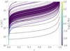 |
Fig. 20. Orbital evolution for merging BHBs in SET10. Each coloured track represents one model, with tracks moving from right to left and from top to bottom. The coloured map labels the BHB frequency. |
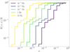 |
Fig. 21. Eccentricity cumulative distribution for all the merging BHBs in model 10. The ef values are calculated as the BHB crosses a given frequency, as indicated in the legend. |
The absence of eccentric sources emitting in the 1−10 Hz band is essentially due to the initial orbital properties of triples. This is clear from Fig. 22, which shows, for the inner BHB, the ratio between the final and initial semi-major axis values and the difference between the final and initial eccentricity. Indeed, although the final BHBs tend to have significantly increased ei values, their semi-major axis decreases only by less than an order of magnitude in most cases, where af ≳ 10−3 AU and fGW ∼ 10−3 − 10−1 Hz. Interestingly, merging binaries draw a quite clear pattern in the af/a − (ef − e) plane, showing that the BHBs that shrink more (af/ai ≲ 10−2) tend to maintain their initial eccentricity or circularise (ef − ei < 0). We note that these quantities are extracted from the last snapshot of our simulations, and therefore provide information on how stellar dynamics shape the BHB final properties.
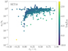 |
Fig. 22. Final to initial inner BHB semi-major axis ratio as a function of the difference between the final and initial BHB eccentricity. All the data points represent binaries that coalesce within 14 Gyr. The colour coded maps identify the binary frequency by the end of our simulations. |
5.2. Gravitational waves from mergers in dense star clusters
To explore whether harder initial BHBs can emit GWs in the Hz regime while having a large eccentricity, we assume l = 100 in the following. This implies, for instance, that circular binaries in the rescaled set have ai = 0.01 AU, thus representing typical values of dense GCs and NCs. We note that the eccentricity distribution remains unaltered, as do the distributions of all the other parameters. This can be easily done in N-body simulations, provided that the length-scale rescaling is associated to a corresponding rescaling of the time unit and the gravitational constant. In this case, as shown in Fig. 23, a sizeable number of binaries cross the Hz band while still having a non-negligible eccentricity.
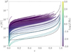 |
Fig. 23. As in Fig. 20, but assuming an initial BHB semi-major axis a = 0.01 AU at zero-eccentricity. |
The eccentricity distribution and the corresponding cumulative distribution for our rescaled systems are shown in Fig. 24. As summarised in Table 6, the percentage of eccentric sources increases from 0.5% to 2%, 7%, 30%, and to 92% at frequencies of 10, 1, 10−1, 10−2, and 10−3 Hz, and therefore almost all mergers appear to be eccentric in the LISA observational band. Our results suggest that hard BHBs ejected in non-hierarchical triples maintain a relatively large eccentricity while passing through the 10−3 − 10−1 Hz frequency range. Hence, these eccentric sources could be observed with DECIGO and LISA, but they become nearly circular by the time they enter the LIGO frequency band because of circularisation caused by GWs (Samsing & D’Orazio 2018). We note that here we consider only mergers with GW time below 14 Gyr. On the other hand, mergers of BHBs with initially smaller semi-major axes (ai ≲ 10−2) have a large probability of entering the fGW ∼ 1 Hz regime with large eccentricities, e > 0.7, and these are possibly observable using the Einstein Telescope in the coming years. Approximately one-third of the BHBs shift from 0.1 Hz toward the LIGO/VIRGO band at ∼10 Hz, with 70% of them having eccentricities above 0.1 as shown in Fig. 23. We note that this plot also suggests that sources possibly drifting toward the LIGO band form with initial eccentricities above ∼5 × 10⁻², implying that they do not cross the LISA observational frequency range, as also suggested by Samsing et al. (2018b).
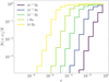 |
Fig. 24. As in Fig. 21, but assuming an initial BHB semi-major axis a = 0.01 AU at zero-eccentricity. |
5.3. Gravitational wave detectability
Following Kocsis et al. (2012), we calculated the characteristic amplitude hc for all the merging BHBs in SET10 in order to determine whether they are visible in low- or high-frequency detectors. As opposed to the assumptions of Sesana (2016), however, our BHBs have eccentric orbits. For sources that do not inspiral significantly during the observation time T, i.e. T < f/ḟp, the GW strain is composed of discrete harmonics with frequency
![$$ \begin{aligned} f_n = n \nu = \frac{n}{2\pi } \left[\frac{G M}{a^{3}}\right]^{1/2}, \end{aligned} $$](/articles/aa/full_html/2021/06/aa38795-20/aa38795-20-eq41.gif)
each of width Δf ∼ 1/T, where ν = a3/2/(GM)1/2 (Peters & Mathews 1963), and

where
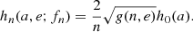
The condition on the inspiral timescale T > fp/ḟp can be calculated using the following relations (Peters 1964) for frequency and its derivative,
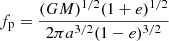
where ȧ and ė are defined in Eq. (16). In the equations above, h0 is the characteristic strain for a circular source (O’Leary et al. 2009; Kocsis et al. 2012; Sesana 2016)
D is the distance of the source, a the binary semi-major axis, and Mz = (1 + z)(M1 + M2) and μz = M1M2/(M1 + M2) are the total and reduced binary masses, respectively, where z is the cosmological redshift.
The function g(e, n) in Eq. (32) is defined as (Peters & Mathews 1963; O’Leary et al. 2009; Kocsis et al. 2012; Gondán et al. 2018b)
![$$ \begin{aligned} g(e,n) =&\frac{n^4}{32} \left[\left(J_{n-2}-2eJ_{n-1}+\frac{2}{n}J_n+2eJ_{n+1}-J_{n+2}\right)^2\right.\nonumber \\&\left.+ \left(1-e^2\right)\left(J_{n-2}-2J_n+J_{n+2}\right)^2 + \frac{4}{3n^2}J_n^2\right], \end{aligned} $$](/articles/aa/full_html/2021/06/aa38795-20/aa38795-20-eq48.gif)
where Ji ≡ Ji(x) is the ith Bessel function evaluated at x = ne (Peters & Mathews 1963). The dominant frequency harmonic corresponds to fp = np(1 − e)3/2ν, with (O’Leary et al. 2009; Kocsis et al. 2012)
![$$ \begin{aligned} n_{\rm p}(e) = \mathrm{ceil}\left[1.15\frac{(1+e)^{1/2}}{(1-e)^{3/2}}\right], \end{aligned} $$](/articles/aa/full_html/2021/06/aa38795-20/aa38795-20-eq49.gif)
where ceil[x] is the nearest integer larger than x, and 90% of the GW power is emitted at frequencies between 0.2fp and 3fp (O’Leary et al. 2009), while it rapidly decreases as the frequency moves away from these limiting values.
For a non-inspiraling eccentric source, the characteristic strain in each frequency bin Δf is given by (Kocsis et al. 2012)
where T is the observation time and
Figure 25 shows how the fundamental frequency, the corresponding characteristic strain, and the eccentricity vary for 150 mergers in SET10. For clarity, we do not show other harmonics in the same plot, despite the fact that the signal is initially broadband. Nevertheless, for each binary we do calculate the contribution of all the collective harmonics, which contribute 90% of the total GW emitting power (O’Leary et al. 2009; Kocsis et al. 2012). We assumed a T = 4 yr observation time and used Eq. (39) for a non-inspiraling source. However, for binaries with an inspiral timescale in the range fp/ḟp < T, we scaled the characteristic strain of each binary by a factor  in order to compensate for the fact that the binary has a limited lifetime at the characteristic frequency and the corresponding characteristic strain is suppressed. This is a conservative estimate for eccentric orbits, because in reality the binary circularises and emits GWs not only during pericentral passage, but throughout the orbit.
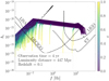 |
Fig. 25. Characteristic strain amplitude evolution for the dominant frequency of 150 merging BHBs in SET10 compared with the sensitivity curves for LISA, KAGRA, LIGO, DECIGO and the Einstein Telescope GW observatories. The coloured map identifies BHB eccentricity. |
The sources are all assumed to be at a luminosity distance DL = 477 Mpc and redshift z = 0.1. These tracks show approximately how the characteristic strain evolves as the binaries shrink and merge. The turning point evident in all the curves marks a time-to-merger of 4 yr. We note that LISA (Robson et al. 2019; Larson et al. 2000), LIGO2, KAGRA3, DECIGO (adapted from Yagi & Seto 2011) and the Einstein Telescope (Hild et al. 2008; Punturo et al. 2010) sensitivity curves are also shown in Fig. 25. Many sources fall in the observational LISA band at formation with high eccentricity. All stellar mass sources that merge within a Hubble time become potentially observable with LIGO, VIRGO, and KAGRA. These sources are more circular; in this case the characteristic strain in Fig. 25 follows f−1/6. The final phase is described with a simple PhenomA prescription as described in Robson et al. (2019).
Such a finding could help in disentangling the origin of observed GW sources. From Eq. (33) we can calculate the semi-major axis of a BHB with a given eccentricity and emitting at a given frequency:
which implies that circular BHBs visible in the LISA frequency band have an aGW value that is two or three orders of magnitude larger than those visible in the LIGO band. For reference, we note that a circular BHB with mass MBHB = 20 M⊙ emitting at a peak frequency of 1 mHz has a semi-major axis aGW = 0.003 AU, while a BHB with an eccentricity eGW > 0.999 emitting at the same peak frequency has aGW < 3.9 AU. Figure 26 shows the evolution of semi-major axis and eccentricity during the BHB inspiral assuming two different setups: (a) BHB mass MBHB = 79.4 M⊙, eccentricity e = 0.947, and semi-major axis a = 0.014 − 0.14 − 1.4 AU; and (b) BHB mass MBHB = 80 M⊙, eccentricity e = 0.999, and semi-major axis a = 0.044 − 0.44 − 4.44. The two panels highlight the importance of measuring the BHB eccentricity with high precision to gain insight into the BHB properties at the time when it ‘decouples’ from the dynamics of the nursing environment. For instance, measuring a BHB mass ∼80 M⊙ and an eccentricity eHz ∼ 0.1 at 1 Hz would imply that the BHB was extremely eccentric and tight at the time of decoupling (a < 0.1 AU and e ∼ 0.999), suggesting an extremely dense birth site. Such tight and eccentric binaries would be undetected by LISA but might be clearly visible with DECIGO and DOs, as shown in Fig. 25. Nonetheless, LISA might help in gaining insight into the origin of BHB mergers that appear completely circular in LIGO and DECIGO. Observing a BHB with mass ∼75 M⊙ and e ≳ 0.1 at 1 mHz, for instance, would lead to decoupling parameters of a ∼ 0.1 AU and e ∼ 0.95, while if the source appears circular in LISA its decoupling semi-major axis would increase by up to an order of magnitude. From Eqs. (28) and (29), the typical semi-major axis of ejected BHB mergers in dense clusters can be written as:
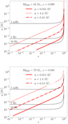 |
Fig. 26. Top panel: semi-major axis–eccentricity evolution for two inspiral BHBs with mass MBHB = 80 M⊙, eccentricity e = 0.999, and corresponding semi-major axis a = 0.044 AU (dotted red line), 0.44 AU (dotted-dashed red line), or 4.4 AU (straight red line). The dashed black line marks the locus of (a, e) for which the peak frequency is 10−3 to 1 − 10 Hz. Bottom panel: same as top panel, but the binary has a mass MBHB = 79 M⊙, eccentricity e = 0.947, and semi-major axis a = 0.014, 0.14, or 1.4 AU. |
Comparing with Fig. 26, for a normal globular cluster (σ ∼ 5 km s−1), a typical ejected merger with a mass ∼80 M⊙ and high eccentricity (e ≃ 0.95) has ae ∼ 1.8 AU and will appear already circular in LISA, whereas in the case of a nuclear cluster (σ ∼ 20 km s−1) the same binary would have ae ∼ 0.11 AU, and might therefore preserve a sizeable eccentricity while transiting in the LISA band. Although rough, this line of thinking provides a link between the observed GW signal, in particular the eccentricity, and the properties of BHB mergers forming dynamically in star clusters. LISA will provide a view of eccentric mergers forming in low-velocity dispersion, that is, in low-density clusters, whereas LIGO, Virgo, KAGRA, and, in the future, ET, can be used to gather information on eccentric mergers developing in massive and dense globular clusters and galactic nuclei.
6. Conclusion
In this paper we investigate the formation, evolution, and merger of BHBs formed in triples produced via BHB–BHB scattering in star clusters. Using 32 000 three-body simulations, we explored the parameter space by varying orbital parameters and initial configuration focusing our attention on the role played by the inclination of the outer perturber in the evolution of the BHB, and in particular on the differences between prograde and retrograde configurations. Furthermore, we discuss the implications for BHB coalescence in the context of GW emission and detection. Our main results can be summarised as follows.
-
We exploit the MOCCA Survey Database I –a suite of Monte Carlo simulations of GCs– to quantify the occurrence rate of BHB–BHB scattering in GCs. We find that, on average, GCs can harbour 103 binary–binary scatterings over a 12 Gyr lifetime, with denser clusters hosting more scattering events (Fig. 1).
-
We use 2000 N-body simulations to model strong BHB–BHB scatterings while varying the host cluster velocity dispersion. Our simulations suggest that this class of interactions trigger the formation of either stable or temporary bound triples whose evolution can in some cases ultimately lead to the formation of a merging BHB. Around (30−40)% of triples formed in this way are unstable, while in several models the newly formed triple arranges in a hierarchical configuration that undergoes KL oscillations. Depending on the cluster velocity dispersion, in 0.6 − 10% of the cases, the BHB–BHB scattering and subsequent formation of short- or long-lived triples drives the formation of a BHB merger (see Figs. 2–6 and Table 1).
-
We perform 1000 simulations (SET0) of triples with initial conditions drawn according to the BHB–BHB scattering experiments, assuming a cluster velocity dispersion of 15 km s−1. We find a BHB merger probability of 22.7% either developing in hierarchical, mildy hierarchical (20.8%), or unstable (1.9%) triples. Under astrophysically motivated assumptions, we find that mergers developing this way have masses in the range MBHB = 30 − 40 M⊙ and mass ratios peaking at qBHB = 0.6. Interestingly, we find that triples tend to evolve toward prograde configuration, with the retrograde ones prone to flipping. Most of the mergers develop in triples characterised by an inclination close to 90° (Figs. 7–10).
-
For all mergers in SET0, we reconstruct the evolution of the orbital properties during the inspiral phase. We find that up to 20% of the mergers retain an eccentricity above 0.1 when emitting GW at 1 mHz (the LISA observational domain), while the fraction of eccentric sources drops to 2% if we consider sources emitting at 1 Hz. Around 75% of mergers developing from non-hierarchical triples are eccentric in the LISA band (Fig. 11).
-
To investigate the role of the triple configuration in the development of mergers, we carry out a suite of 14 000 three-body simulations tailored to exploring different properties of BH triples initially in the non-hierarchical regime. Our results suggest that non-hierarchical triples share three evolutionary features: (a) triple systems tend to evolve toward co-rotation, (b) the orbital flip causes the formation of a tighter inner BHB, and (c) coplanar retrograde systems have 2.5 times greater chance of decreasing the inner BHB merger time by a factor of 100 than coplanar prograde systems (Figs. 17 and 18 and Tables 4 and 5).
-
We perform 16 000 three-body models to investigate the role of BH masses in the case of an inner BHB with semi-major axis of a = 1 − 20 AU (8000 simulations each). In the case of a loose BHB, we find only 15 mergers out of 8000 simulations (merger probability 0.25%), while the number increased to 677 (8.5%) in the case of an initially tighter binary. The majority of mergers (around two-thirds) occur in triples with an initially retrograde configuration. The merger time distribution follows a clear power law:
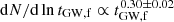 (Fig. 14).
 -
Taking advantage of a convenient scaling of the simulations result, we explore the differences in the GW signal produced by merging binaries produced in triples with an inner BHB semi-major axis of a = 0.01 − 1 AU. We find a non-negligible number of mergers that retain a significant eccentricity during the different phases of the inspiral. In the case of triples with an initially loose BHB, ∼17% of mergers have eccentricity > 0.1 when the emitted GW signal has a peak frequency of 1 mHz, but only 0.2% are eccentric in the Hz, and none of them in the 10 Hz. Initially tight BHBs, instead, appear eccentric in the mHz band in 92% of cases, and appear eccentric in the 10 Hz band in 0.5% of cases (Figs. 22 and 25, and Table 6).
-
We calculate the GW characteristic strain for merging BHBs and make a comparison with the sensitivity curve of several GW detectors, showing that the vast majority of mergers can be multiband sources, that is, sources detectable with more than one detector (Fig. 25).
-
We show that precise measurements of merger eccentricity can enable us to dissect the merger evolutionary history. Depending on BHB mass and the eccentricity measured in a given frequency band, we suggest that it is possible to decipher whether the merger formed in a low- or high-velocity dispersion environment. For instance, a BHB merger with mass ∼80 M⊙ observed in LISA with eccentricity > 0.1 would suggest an orbital semi-major axis at ‘formation’ of a ∼ 0.1 AU, a value typical of mergers ejected in clusters with a velocity dispersion of ∼20 km s−1 (Fig. 26). Our simulations show that the chaotic evolution of mildly hierarchical and unstable BH triples in dense clusters can be broadly described as a function of the initial orbital configuration of the triple: (i) Retrograde triples evolve toward a prograde configuration, whilst this orbital flip is less frequent for initially prograde triples. (ii) Flipping systems lead on average to tighter BHBs. (iii) Exactly prograde triples are most likely to produce merging BHBs. The occurrence of such general results depends critically on the mechanisms that regulate the triple BH formation, particularly the orbital parameters of BHB–BHB scatterings, the star cluster velocity dispersion, and the BH mass spectrum. We show that the evolution of triple BHs in compact and dense star clusters (like globular and nuclear clusters) are more likely to produce BHB mergers audible to ground-based GW detectors, whilst those developing in looser clusters (like young and open clusters) lead on average to GW sources that are potentially detectable by space-borne detectors. The future synergy between ground-based detectors, like the Einstein Telescope or the Cosmic Explorer, and space-based observatories, like LISA or DECIGO, will therefore provide us with a unique view OF the variety of dynamical environments that could trigger BHB mergers from unstable triples.
Acknowledgments
MAS acknowledges the Sonderforschungsbereich SFB 881 “The Milky Way System” (subproject Z2) of the German Research Foundation (DFG) for the financial support provided. MAS also acknowledges financial support from the Alexander von Humboldt Foundation and the Federal Ministry for Education and Research in the framework of the research project “The evolution of black holes from stellar to galactic scales”. The authors warmly thank Abbas Askar and Mirek Giersz for useful discussions and for their help with MOCCA data handling and analysis. The authors thank Hagai Perets and Yann Gao for useful discussions. This project benefited from support by the International Space Science Institute, Bern, Switzerland, through its International Team programme ref. no. 393 “The Evolution of Rich Stellar Populations and BH Binaries” (2017-18). This project has received funding from the European Research Council (ERC) under the European Union’s Horizon 2020 research and innovation programme ERC-2014-STG under grant agreement No 638435 (GalNUC) (to B.K.).
References
- Aasi, J., Abbott, B. P., & Abbott, R. 2015, Classical Quantum Gravity, 32, 074001 [NASA ADS] [CrossRef] [Google Scholar]
- Abbott, B. P., Abbott, R., Abbott, T. D., et al. 2016a, Phys. Rev. D, 93, 122003 [NASA ADS] [CrossRef] [Google Scholar]
- Abbott, B. P., Abbott, R., Abbott, T. D., et al. 2016b, Phys. Rev. Lett., 116, 061102 [Google Scholar]
- Abbott, B. P., Abbott, R., Abbott, T. D., et al. 2016c, Phys. Rev. Lett., 116, 241103 [Google Scholar]
- Abbott, B. P., Abbott, R., Abbott, T. D., et al. 2017a, Phys. Rev. Lett., 118, 221101 [NASA ADS] [CrossRef] [PubMed] [Google Scholar]
- Abbott, B. P., Abbott, R., Abbott, T. D., et al. 2017b, Phys. Rev. Lett., 119, 141101 [Google Scholar]
- Abbott, R., Abbott, T. D., Abraham, S., et al. 2020, ArXiv e-prints [arXiv:2010.14527] [Google Scholar]
- Acernese, F., Agathos, M., Agatsuma, K., et al. 2015, Classical Quantum Gravity, 32, 024001 [NASA ADS] [CrossRef] [Google Scholar]
- Akutsu, T., Ando, M., Arai, K., et al. 2019, Nat. Astron., 3, 35 [NASA ADS] [CrossRef] [Google Scholar]
- Amaro-Seoane, P., Audley, H., Babak, S., et al. 2017, ArXiv e-prints [arXiv:1702.00786] [Google Scholar]
- Antonini, F., & Perets, H. B. 2012, ApJ, 757, 27 [NASA ADS] [CrossRef] [Google Scholar]
- Antonini, F., & Rasio, F. A. 2016, ApJ, 831, 187 [NASA ADS] [CrossRef] [Google Scholar]
- Antonini, F., Murray, N., & Mikkola, S. 2014, ApJ, 781, 45 [NASA ADS] [CrossRef] [Google Scholar]
- Antonini, F., Chatterjee, S., Rodriguez, C. L., et al. 2016, ApJ, 816, 65 [NASA ADS] [CrossRef] [Google Scholar]
- Antonini, F., Toonen, S., & Hamers, A. S. 2017, ApJ, 841, 77 [NASA ADS] [CrossRef] [Google Scholar]
- Arca-Sedda, M. 2016, MNRAS, 455, 35 [NASA ADS] [CrossRef] [Google Scholar]
- Arca Sedda, M. 2020, Commun. Phys., 3, 43 [CrossRef] [Google Scholar]
- Arca Sedda, M., & Benacquista, M. 2019, MNRAS, 482, 2991 [NASA ADS] [Google Scholar]
- Arca-Sedda, M., & Capuzzo-Dolcetta, R. 2019, MNRAS, 483, 152 [NASA ADS] [CrossRef] [Google Scholar]
- Arca Sedda, M., Askar, A., & Giersz, M. 2018, MNRAS, 479, 4652 [NASA ADS] [CrossRef] [Google Scholar]
- Arca-Sedda, M., Kocsis, B., & Brandt, T. D. 2018, MNRAS, 479, 900 [NASA ADS] [CrossRef] [Google Scholar]
- Arca Sedda, M., Mapelli, M., Spera, M., Benacquista, M., & Giacobbo, N. 2020a, ApJ, 894, 133 [CrossRef] [Google Scholar]
- Arca Sedda, M., Berry, C. P. L., Jani, K., et al. 2020b, Classical Quantum Gravity, 37, 215011 [CrossRef] [Google Scholar]
- Askar, A., Szkudlarek, M., Gondek-Rosińska, D., Giersz, M., & Bulik, T. 2017, MNRAS, 464, L36 [NASA ADS] [CrossRef] [Google Scholar]
- Askar, A., Arca Sedda, M., & Giersz, M. 2018, MNRAS, 478, 1844 [NASA ADS] [CrossRef] [Google Scholar]
- Bacon, D., Sigurdsson, S., & Davies, M. B. 1996, MNRAS, 281, 830 [NASA ADS] [CrossRef] [Google Scholar]
- Baibhav, V., Gerosa, D., Berti, E., et al. 2020, Phys. Rev. D, 102, 043002 [CrossRef] [Google Scholar]
- Banerjee, S. 2017, MNRAS, 467, 524 [NASA ADS] [Google Scholar]
- Banerjee, S. 2018, MNRAS, 473, 909 [NASA ADS] [CrossRef] [Google Scholar]
- Bartos, I., Kocsis, B., Haiman, Z., & Márka, S. 2017, ApJ, 835, 165 [CrossRef] [Google Scholar]
- Belczynski, K., Holz, D. E., Bulik, T., & O’Shaughnessy, R. 2016, Nature, 534, 512 [Google Scholar]
- Belczynski, K., Klencki, J., Meynet, G., et al. 2020, A&A, 636, A104 [CrossRef] [EDP Sciences] [Google Scholar]
- Binney, J., & Tremaine, S. 2008, Galactic Dynamics: Second Edition (Princeton: Princeton University Press) [Google Scholar]
- Blaes, O., Lee, M. H., & Socrates, A. 2002, ApJ, 578, 775 [NASA ADS] [CrossRef] [Google Scholar]
- Breen, P. G., & Heggie, D. C. 2013, MNRAS, 432, 2779 [NASA ADS] [CrossRef] [Google Scholar]
- Chandrasekhar, S. 1943, ApJ, 97, 255 [NASA ADS] [CrossRef] [Google Scholar]
- Contenta, F., Varri, A. L., & Heggie, D. C. 2015, MNRAS, 449, L100 [CrossRef] [Google Scholar]
- Deme, B., Hoang, B.-M., Naoz, S., & Kocsis, B. 2020, ApJ, 901, 125 [CrossRef] [Google Scholar]
- Di Carlo, U. N., Giacobbo, N., Mapelli, M., et al. 2019, MNRAS, 487, 2947 [NASA ADS] [CrossRef] [Google Scholar]
- Downing, J. M. B., Benacquista, M. J., Giersz, M., & Spurzem, R. 2010, MNRAS, 407, 1946 [NASA ADS] [CrossRef] [Google Scholar]
- Fragione, G., & Kocsis, B. 2018, Phys. Rev. Lett., 121, 161103 [Google Scholar]
- Fragione, G., Loeb, A., & Rasio, F. A. 2020a, ApJ, 902, L26 [CrossRef] [Google Scholar]
- Fragione, G., Martinez, M. A. S., Kremer, K., et al. 2020b, ApJ, 900, 16 [CrossRef] [Google Scholar]
- Fregeau, J. M., Cheung, P., Portegies Zwart, S. F., & Rasio, F. A. 2004, MNRAS, 352, 1 [NASA ADS] [CrossRef] [Google Scholar]
- Gayathri, V., Bartos, I., Haiman, Z., et al. 2020, ApJ, 890, L20 [CrossRef] [Google Scholar]
- Gerosa, D., & Berti, E. 2017, Phys. Rev. D, 95, 124046 [NASA ADS] [CrossRef] [Google Scholar]
- Giersz, M., Leigh, N., Hypki, A., Lützgendorf, N., & Askar, A. 2015, MNRAS, 454, 3150 [NASA ADS] [CrossRef] [Google Scholar]
- Gondán, L., & Kocsis, B. 2019, ApJ, 871, 178 [CrossRef] [Google Scholar]
- Gondán, L., Kocsis, B., Raffai, P., & Frei, Z. 2018a, ApJ, 860, 5 [CrossRef] [Google Scholar]
- Gondán, L., Kocsis, B., Raffai, P., & Frei, Z. 2018b, ApJ, 855, 34 [CrossRef] [Google Scholar]
- Grishin, E., Perets, H. B., Zenati, Y., & Michaely, E. 2017, MNRAS, 466, 276 [NASA ADS] [CrossRef] [Google Scholar]
- Grishin, E., Perets, H. B., & Fragione, G. 2018, MNRAS, 481, 4907 [NASA ADS] [CrossRef] [Google Scholar]
- Harrington, R. S. 1968, AJ, 73, 190 [NASA ADS] [CrossRef] [Google Scholar]
- Heggie, D. C. 1975, MNRAS, 173, 729 [NASA ADS] [CrossRef] [Google Scholar]
- Hild, S., Chelkowski, S., & Freise, A. 2008, ArXiv e-prints [arXiv:0810.0604] [Google Scholar]
- Hoang, B.-M., Naoz, S., Kocsis, B., Rasio, F. A., & Dosopoulou, F. 2018, ApJ, 856, 140 [NASA ADS] [CrossRef] [Google Scholar]
- Hoang, B.-M., Naoz, S., Kocsis, B., Farr, W., & McIver, J. 2019, ApJ, 875, L31 [CrossRef] [Google Scholar]
- Hollywood, J. M., & Melia, F. 1997, ApJS, 112, 423 [NASA ADS] [CrossRef] [Google Scholar]
- Hut, P., & Bahcall, J. N. 1983, ApJ, 268, 319 [NASA ADS] [CrossRef] [Google Scholar]
- Hut, P., McMillan, S., Goodman, J., et al. 1992, PASP, 104, 981 [NASA ADS] [CrossRef] [Google Scholar]
- Hypki, A., & Giersz, M. 2013, MNRAS, 429, 1221 [NASA ADS] [CrossRef] [Google Scholar]
- Jeans, J. H. 1919, MNRAS, 79, 408 [NASA ADS] [CrossRef] [Google Scholar]
- Katz, B., Dong, S., & Malhotra, R. 2011, Phys. Rev. Lett., 107, 181101 [NASA ADS] [CrossRef] [Google Scholar]
- Kawamura, S., Ando, M., Seto, N., et al. 2011, Classical Quantum Gravity, 28, 094011 [NASA ADS] [CrossRef] [Google Scholar]
- Kimball, C., Talbot, C., Berry, C. P. L., et al. 2020, ArXiv e-prints [arXiv:2011.05332] [Google Scholar]
- Kocsis, B., Ray, A., & Portegies Zwart, S. 2012, ApJ, 752, 67 [CrossRef] [Google Scholar]
- Kozai, Y. 1962, AJ, 67, 591 [Google Scholar]
- Kremer, K., Ye, C. S., Rui, N. Z., et al. 2020, ApJS, 247, 48 [CrossRef] [Google Scholar]
- Kulkarni, S. R., Hut, P., & McMillan, S. 1993, Nature, 364, 421 [NASA ADS] [CrossRef] [Google Scholar]
- Kumamoto, J., Fujii, M. S., & Tanikawa, A. 2019, MNRAS, 486, 3942 [CrossRef] [Google Scholar]
- Larson, S. L., Hiscock, W. A., & Hellings, R. W. 2000, Phys. Rev. D, 62, 062001 [NASA ADS] [CrossRef] [Google Scholar]
- Li, G., Naoz, S., Kocsis, B., & Loeb, A. 2014, ApJ, 785, 116 [NASA ADS] [CrossRef] [Google Scholar]
- Li, G., Hadden, S., Payne, M., & Holman, M. J. 2018, AJ, 156, 263 [CrossRef] [Google Scholar]
- Lidov, M. L. 1962, Planet. Space Sci., 9, 719 [Google Scholar]
- Lithwick, Y., & Naoz, S. 2011, ApJ, 742, 94 [NASA ADS] [CrossRef] [Google Scholar]
- LIGO Scientific Collaboration & Virgo Collaboration (Abbott, B. P., et al.) 2019, Phys. Rev. X, 9, 031040 [Google Scholar]
- LIGO Scientific Collaboration & Virgo Collaboration (Abbott, R., et al.) 2021, ApJ, 913, L7 [CrossRef] [Google Scholar]
- Liu, B., & Lai, D. 2021, MNRAS, 502, 2049 [CrossRef] [Google Scholar]
- Manwadkar, V., Kol, B., Trani, A. A., & Leigh, N. W. C. 2021, ArXiv e-prints [arXiv:2101.03661] [Google Scholar]
- Mapelli, M. 2016, MNRAS, 459, 3432 [NASA ADS] [CrossRef] [Google Scholar]
- Mardling, R. A., & Aarseth, S. J. 2001, MNRAS, 321, 398 [NASA ADS] [CrossRef] [Google Scholar]
- Martinez, M. A. S., Fragione, G., Kremer, K., et al. 2020, ApJ, 903, 67 [CrossRef] [Google Scholar]
- McMillan, S., Hut, P., & Makino, J. 1991, ApJ, 372, 111 [NASA ADS] [CrossRef] [Google Scholar]
- Meiron, Y., Kocsis, B., & Loeb, A. 2017, ApJ, 834, 200 [CrossRef] [Google Scholar]
- Mikkola, S. 1984, MNRAS, 207, 115 [CrossRef] [Google Scholar]
- Mikkola, S., & Merritt, D. 2008, AJ, 135, 2398 [Google Scholar]
- Mikkola, S., & Tanikawa, K. 1999, MNRAS, 310, 745 [CrossRef] [Google Scholar]
- Mikóczi, B., Kocsis, B., Forgács, P., & Vasúth, M. 2012, Phys. Rev. D, 86, 104027 [CrossRef] [Google Scholar]
- Miller, M. C., & Hamilton, D. P. 2002, ApJ, 576, 894 [NASA ADS] [CrossRef] [Google Scholar]
- Miller, M. C., & Lauburg, V. M. 2009, ApJ, 692, 917 [NASA ADS] [CrossRef] [Google Scholar]
- Morscher, M., Pattabiraman, B., Rodriguez, C., Rasio, F. A., & Umbreit, S. 2015, ApJ, 800, 9 [NASA ADS] [CrossRef] [Google Scholar]
- Naoz, S. 2016, ARA&A, 54, 441 [Google Scholar]
- Naoz, S., Farr, W. M., Lithwick, Y., Rasio, F. A., & Teyssandier, J. 2011, Nature, 473, 187 [NASA ADS] [CrossRef] [Google Scholar]
- Naoz, S., Farr, W. M., Lithwick, Y., Rasio, F. A., & Teyssandier, J. 2013a, MNRAS, 431, 2155 [NASA ADS] [CrossRef] [Google Scholar]
- Naoz, S., Kocsis, B., Loeb, A., & Yunes, N. 2013b, ApJ, 773, 187 [NASA ADS] [CrossRef] [Google Scholar]
- O’Leary, R. M., Rasio, F. A., Fregeau, J. M., Ivanova, N., & O’Shaughnessy, R. 2006, ApJ, 637, 937 [NASA ADS] [CrossRef] [Google Scholar]
- O’Leary, R. M., Kocsis, B., & Loeb, A. 2009, MNRAS, 395, 2127 [NASA ADS] [CrossRef] [Google Scholar]
- O’Leary, R. M., Meiron, Y., & Kocsis, B. 2016, ApJ, 824, L12 [CrossRef] [Google Scholar]
- Panamarev, T., Just, A., Spurzem, R., et al. 2019, MNRAS, 484, 3279 [CrossRef] [Google Scholar]
- Pattabiraman, B., Umbreit, S., Liao, W.-K., et al. 2013, ApJS, 204, 15 [NASA ADS] [CrossRef] [Google Scholar]
- Peters, P. C. 1964, Phys. Rev., 136, B1224 [NASA ADS] [CrossRef] [Google Scholar]
- Peters, P. C., & Mathews, J. 1963, Phys. Rev., 131, 435 [NASA ADS] [CrossRef] [Google Scholar]
- Pooley, D., Lewin, W. H. G., Anderson, S. F., et al. 2003, ApJ, 591, L131 [NASA ADS] [CrossRef] [Google Scholar]
- Portegies Zwart, S. F., & McMillan, S. L. W. 2000, ApJ, 528, L17 [NASA ADS] [CrossRef] [Google Scholar]
- Punturo, M., Abernathy, M., Acernese, F., et al. 2010, Classical Quantum Gravity, 27, 194002 [NASA ADS] [CrossRef] [Google Scholar]
- Randall, L., & Xianyu, Z. Z. 2019, ArXiv e-prints [arXiv:1902.08604] [Google Scholar]
- Rastello, S., Amaro-Seoane, P., Arca-Sedda, M., et al. 2019, MNRAS, 483, 1233 [NASA ADS] [CrossRef] [Google Scholar]
- Rastello, S., Mapelli, M., Di Carlo, U. N., et al. 2020, MNRAS, 497, 1563 [CrossRef] [Google Scholar]
- Robson, T., Cornish, N. J., & Liu, C. 2019, Classical Quantum Gravity, 36, 105011p [NASA ADS] [CrossRef] [Google Scholar]
- Rodriguez, C. L., & Antonini, F. 2018, ApJ, 863, 7 [NASA ADS] [CrossRef] [Google Scholar]
- Rodriguez, C. L., Morscher, M., Pattabiraman, B., et al. 2015, Phys. Rev. Lett., 115, 051101 [NASA ADS] [CrossRef] [Google Scholar]
- Rodriguez, C. L., Chatterjee, S., & Rasio, F. A. 2016, Phys. Rev. D, 93, 084029 [NASA ADS] [CrossRef] [Google Scholar]
- Rodriguez, C. L., Amaro-Seoane, P., Chatterjee, S., et al. 2018, Phys. Rev. D, 98, 123005 [NASA ADS] [CrossRef] [Google Scholar]
- Samsing, J., & D’Orazio, D. J. 2018, MNRAS, 481, 5445 [CrossRef] [Google Scholar]
- Samsing, J., & Ilan, T. 2018, MNRAS, 476, 1548 [CrossRef] [Google Scholar]
- Samsing, J., MacLeod, M., & Ramirez-Ruiz, E. 2014, ApJ, 784, 71 [CrossRef] [Google Scholar]
- Samsing, J., Askar, A., & Giersz, M. 2018a, ApJ, 855, 124 [CrossRef] [Google Scholar]
- Samsing, J., D’Orazio, D. J., Askar, A., & Giersz, M. 2018b, ArXiv e-prints [arXiv:1802.08654] [Google Scholar]
- Sesana, A. 2016, Phys. Rev. Lett., 116, 231102 [NASA ADS] [CrossRef] [PubMed] [Google Scholar]
- Sigurdsson, S., & Hernquist, L. 1993, Nature, 364, 423 [NASA ADS] [CrossRef] [Google Scholar]
- Sippel, A. C., & Hurley, J. R. 2013, MNRAS, 430, L30 [NASA ADS] [Google Scholar]
- Sippel, A. C., Hurley, J. R., Madrid, J. P., & Harris, W. E. 2012, MNRAS, 427, 167 [NASA ADS] [CrossRef] [Google Scholar]
- Spitzer, L., Jr. 1940, MNRAS, 100, 396 [NASA ADS] [CrossRef] [Google Scholar]
- Tagawa, H., Haiman, Z., & Kocsis, B. 2020a, ApJ, 898, 25 [CrossRef] [Google Scholar]
- Tagawa, H., Haiman, Z., Bartos, I., & Kocsis, B. 2020b, ApJ, 899, 26 [Google Scholar]
- Toonen, S., Hamers, A., & Portegies Zwart, S. 2016, Comput. Astrophys. Cosmol., 3, 6 [CrossRef] [Google Scholar]
- Wang, L., Spurzem, R., Aarseth, S., et al. 2016, MNRAS, 458, 1450 [NASA ADS] [CrossRef] [Google Scholar]
- Weatherford, N. C., Chatterjee, S., Rodriguez, C. L., & Rasio, F. A. 2018, ApJ, 864, 13 [NASA ADS] [CrossRef] [Google Scholar]
- Weatherford, N. C., Chatterjee, S., Kremer, K., & Rasio, F. A. 2020, ApJ, 898, 162 [CrossRef] [Google Scholar]
- Wen, L. 2003, ApJ, 598, 419 [NASA ADS] [CrossRef] [Google Scholar]
- Yagi, K., & Seto, N. 2011, Phys. Rev. D, 83, 044011 [NASA ADS] [CrossRef] [Google Scholar]
- Yang, Y., Bartos, I., Haiman, Z., et al. 2019a, ApJ, 876, 122 [CrossRef] [Google Scholar]
- Yang, Y., Bartos, I., Gayathri, V., et al. 2019b, Phys. Rev. Lett., 123, 181101 [CrossRef] [Google Scholar]
- Zevin, M., Samsing, J., Rodriguez, C., Haster, C.-J., & Ramirez-Ruiz, E. 2019, ApJ, 871, 91 [NASA ADS] [CrossRef] [Google Scholar]
- Zevin, M., Bavera, S. S., Berry, C. P. L., et al. 2021, ApJ, 910, 152 [Google Scholar]
Appendix A: Stability, hierarchy, and post-Newtonian effects
As discussed in Sect. 3, a triple is, in principle, stable and prone to KL oscillations if the criteria given in Eqs. (6)–(10) are fulfilled. However, while it is true that a stable system is generally hierarchical, the converse need not hold. Figure A.1 shows the quantities Kstaba/a3 and ϵoct/0.1 values for all the triples in SET4. Only 3.4% of all models initially fulfill the two criteria, suggesting that the evolution of the majority of these triples is unstable and determined by chaos. Figure A.2 shows the ratio between the initial value of the outer and inner binary angular momentum L3, i/Li for all the initially retrograde (left panel) and prograde (right panel) models in SET4 as a function of the ratio between the final and initial value of the GW merger timescale. For each model, we also mark the ratio between the initial and final values of the inner binary pericentre. We find that the merger time decreases more, on average, for smaller values of the outer angular momentum compared to the inner binary and in particular retrograde models merge more easily than prograde ones.
 |
Fig. A.1. Initial value of the Kstab parameter normalised to the a3/a ratio (y-axis), and of the ϵKL parameter normalised to 0.1 (x-axis) for models in SET4. The semiplane defined by Kstab < a3/a − ϵKL < 0.1 contains triples in an initially stable configuration possibly prone to eccentric KL effects. Red squares mark the triples in which the inner BHB merges within 14 Gyr. The colour coding marks the ratio between the initial and final value of the merger time, tGW, f/tGW, i. |
 |
Fig. A.2. Ratio between the angular momenta of the outer binary and that of the inner binary is compared to the ratio between the initial and final GW timescale of the inner binary for simulation SET4. The colour coding marks the ratio between the final and the initial pericentre for the inner binary. Left (right) panel: refers to prograde(retrograde) models. The GW timescale may change significantly for a broad range of angular momentum ratios, but the distribution is more skewed to lower GW timescales for retrograde orbits. |
This is in agreement with the qualitative arguments discussed in the Sect. 4.1. Figure A.3 shows the final binding energy of the inner binary normalised to its initial value, as a function of the ratio between the inner and outer semi-major axis at time zero. The binding energy of the inner binary can be seen to typically increase during the evolution by up to a factor 1000.
 |
Fig. A.3. Ratio between the final and initial value of the inner binary binding energy as a function of the ratio between the initial inner and outer semi-major axis. The colour-coding marks the ratio between the final and initial values of the coalescence timescale. |
If the inner BHB is sufficiently tight, general relativity (GR) effects have an important influence. However, we find that none of the triples in SET4 satisfy the condition for GR effects to be important. For instance GR precession can suppress KL oscillation if its typical timescale is shorter than the KL timescale (Hollywood & Melia 1997; Blaes et al. 2002; Antonini & Perets 2012; Naoz et al. 2013b; Naoz 2016), i.e.:
![$$ \begin{aligned}&t_{\rm 1PN} = \frac{2\pi a_{\rm i}^{5/2} c^2 (1-e_{\rm i}^2) }{3 [G(M_{\rm 1,i}+M_{\rm 2,i})]^{3/2}} \end{aligned} $$](/articles/aa/full_html/2021/06/aa38795-20/aa38795-20-eq56.gif)
In model SET4, none of the triples satisfy the limit t1PN < tquad, as shown in Fig. A.4, and therefore we expect that GR effects are negligible in affecting the BHB evolution in this type of BH triple.
 |
Fig. A.4. Initial value of the precession time due to GR according to 1PN terms (y-axis) compared with the quadrupole timescale (x-axis) for all models in SET4. The dotted line represents the locus of points having x = y. |
Appendix B: Eccentricity evolution
Another parameter that can be checked to obtain a clearer overview on the triple evolution is the evolution of the maximum value of the eccentricity emax. Figure B.1 shows how the maximum eccentricity varies with the final and initial inclination. The evolution of the triple leads to a decrease of models characterised by high inclinations and low eccentricities, leading to a more efficient population of high eccentricity states. Looking at Fig. B.2, which shows how the ratio between initial and final values of the inclination varies at increasing emax, we note that emax ≃ 0.2 marks a threshold above which the triple configuration changes significantly over time and undergoes, in some cases, a flip. We also note that emax is linked to the ratio (1 − e3)/(1 − e).
 |
Fig. B.1. Maximum eccentricity as a function of the initial (top panel) and final (bottom panel) inclination. The colour-coded map represents the mass of the outer BH. |
 |
Fig. B.2. Ratio between the initial and final value of the cosine of the inclination as a function of the maximum inner eccentricity. The colour coding identifies the ratio between the BHB final and initial values of 1 − e. |
Figure B.3 shows the time evolution of one of the simulations in SET4. Here the outer binary orbit has an initial inclination i = 90° and eccentricity e3 ∼ 0.35, while the inner binary has eccentricity e ≃ 0.4. The ratio between the inner and outer semi-major axis is, in this case, a/a3 = 0.17. The perturbation induced by the outer objects causes an oscillation in e, whose periodicity roughly doubles in the last stage before the merger event. The merger is extremely fast, taking place within ∼5.6 × 10⁴ yr. Also the inclination varies significantly until the merger. The inner binary evolution draws a clear pattern in the e − i plane, as shown in Fig. B.4, with the inclination that continuously flips from a co- to a counter-rotating configuration as the inner eccentricity approaches unity. The boundaries of Fig. B.4, showing how the inclination and eccentricities of the inner binary relate to each other, are obtained assuming a constant value for the z component of the angular momentum 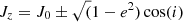 , as expected for standard Kozai-Lidov oscillations. We note that our models start initially on a nearly perpendicular configuration (cos(i) ∼ 0).
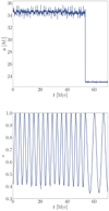 |
Fig. B.3. Top panel: time evolution of a in simulation No. 593 in SET4. Bottom panel: same as in top panel, but here the eccentricity is represented. We note the moment at which the shrinking efficiency peaks at ∼0.05 Myr, after which the semi-major axis drops, the minimum eccentricity decreases, and the eccentricity variation period increases until the merger occurs at 0.07 Myr. |
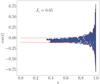 |
Fig. B.4. Inclination as a function of the eccentricity in model No. 593 in SET4. |
All Tables
Fraction of mergers with eccentricity > 0.1 in different frequency bands for SET10.
All Figures
|
Fig. 1. Total number of BHB–BHB interactions as a function of the central density of the host GC at 12 Gyr in the MOCCA database. Colour coding shows the mass of the BH subsystem in the host globular cluster core. |
| In the text | |
|
Fig. 2. Binary–binary interaction in one of the cases investigated. After the close encounter, one BH is ejected and the remaining three BHs form an unstable triple. |
| In the text | |
|
Fig. 3. Top figure: distribution of semi-major axis for the resulting outer (filled blue steps) and inner binaries (filled green steps) following the binary–binary scatterings. Bottom figure: eccentricity distribution of the outer and inner binary, using the same colour-coding as in the top figure. In both figures, panels from top to bottom refer to cluster velocity dispersion values σc = 5 − 10 − 15 km s−1, respectively. |
| In the text | |
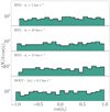 |
Fig. 4. Mutual inclination distribution for the simulations shown in Fig. 3. |
| In the text | |
|
Fig. 5. Surface number density for the stability and octupole-level approximation criteria for triples formed in model BIN2. The two dotted lines delimit regions where the effect of octupole level approximation can become important (left side of the vertical line) or the triple is stable according to the Mardling & Aarseth (2001) criterion (upper side of the horizontal line). |
| In the text | |
|
Fig. 6. Top panel: time evolution of the inner binary eccentricity in the simulated triple BIN1-374. At ∼460 yr, the binary–binary scattering drives the formation of a triple arranged in a hierarchical configuration, while the fourth object is ejected away. KL oscillations are apparent after the formation of the triple system. Bottom panel: same as above, but for model BIN2-152. In this case, the rapid variations are due to the chaotic interaction with the outer perturber, itself attributable to the formation of a non-hierarchical triple. In both cases, colour-coding marks the mutual inclination. |
| In the text | |
|
Fig. 7. Eccentricity variation as a function of time in three systems that lead the inner binary to merge. Top panel: triple in which the inner binary undergoes typical KL oscillations. Central panel: case where KL oscillations vary in phase and amplitude over time. Bottom panel: case of a disrupted triple, with the inner binary evolution driven solely by GW emission. |
| In the text | |
|
Fig. 8. Top panel: initial (red filled boxes) and final (black open steps) inclination distribution for all BHBs in SET0. Bottom panel: same as above, but only for merging BHBs in SET0. |
| In the text | |
|
Fig. 9. Top panel: combined mass distribution of merging BHB components for SET0. The dashed line identifies loci in the plane at a fixed value of the mass ratio. Darker(lighter) colours identify larger(smaller) mass ratios. Bottom panel: mass ratio distribution for merging BHBs in SET0. |
| In the text | |
|
Fig. 10. Cumulative distribution eccentricity (top panel) and its distribution (bottom panel) for all the BHB mergers in model 11. The eccentricity is calculated as the BHB crosses a given frequency, as indicated in the legend. The dotted line indicates a value of eccentricity of e = 0.1. |
| In the text | |
|
Fig. 11. BHB–BH trajectory for a non-hierarchical triple initially in a prograde (top panel) or retrograde (bottom panel) configuration. The time indicated in the figure marks the moment at which the triple breaks up. |
| In the text | |
|
Fig. 12. From top to bottom: semi-major axis and eccentricity of the inner (red solid line) and outer binary (black dotted line) for the triple shown in the bottom panel of Fig. 11. The system shows a bound triple in the first ∼4000 yr, then one object marked with light blue is ejected on a weakly bound eccentric orbit, and is ultimately completely ejected on an unbound trajectory. |
| In the text | |
|
Fig. 13. Initial (filled red boxes) and final (blue steps) GW merger time distribution for all BHBs in SET4 (top panel) and SET10 (bottom panel) (see Table 2 for parameters). The dotted vertical line marks tGW = 14 Gyr. A broad tail extending to low GW timescales is produced with |
| In the text | |
|
Fig. 14. Semi-major axis (left panel) and eccentricity (right panel) distribution for the initial inner BHB population (red filled boxes) and for mergers only (black steps) in SET10. |
| In the text | |
|
Fig. 15. Ratio between the initial and final values of the inner binary pericentre with respect to the outer binary initial separation, normalised to the inner BHB initial semi-major axis, ai = 20 AU. From left to right and from top to bottom panels: SET1 (ei = 0, Δϖi = 0 − 2π, ii = 0°), SET2 (ei = 0, Δϖi = 0, ii = 0 − 10°), SET3 (ei = 0 − 1, Δϖi = 0, ii = 0 − 10°), and SET4 (ei = 0 − 1, Δϖi = 0, ii = 0 − 180°), respectively; see Table 2. The colours represent the ratio between the final and initial value of the GW timescale for the inner binary. Bottom panels: same as in top four panels, but here we show the inner binary final eccentricity vs. the semi-major axis ratio. |
| In the text | |
|
Fig. 16. Percentage of models with ii < Δα (red solid line) or ii > Δα (black dotted line) and tGW, f/tGW, i < 1, 0.1 and 0.01 (from top to bottom) in SET4. Nearly coplanar retrograde orbits have the highest probability of greatly reducing the GW timescale. |
| In the text | |
|
Fig. 17. Initial (filled red steps) and final (empty black steps) inclination distribution in SET4. |
| In the text | |
|
Fig. 18. Final inner binary pericentre as a function of the outer binary initial apocentre, both normalised to the initial pericentre of the inner binary for prograde (SET5, top panel) and retrograde (SET6, bottom panel) systems. Binaries maintaining their original components (10 M⊙ + 20 M⊙) are identified with blue dots, whereas those exchanging the lighter component are shown with green dots and identify final binaries with component masses 20 M⊙ + 20 M⊙. The final binary total mass is identified by the coloured map. |
| In the text | |
|
Fig. 19. Hard binary criterion Γh as a function of the BHB semi-major axis and for different values of the velocity dispersion of the host system, with the upper(lower) limit corresponding to a BHB mass of MBHB = 30(10) M⊙. The horizontal black line marks the boundary between hard and soft binary configurations. |
| In the text | |
|
Fig. 20. Orbital evolution for merging BHBs in SET10. Each coloured track represents one model, with tracks moving from right to left and from top to bottom. The coloured map labels the BHB frequency. |
| In the text | |
|
Fig. 21. Eccentricity cumulative distribution for all the merging BHBs in model 10. The ef values are calculated as the BHB crosses a given frequency, as indicated in the legend. |
| In the text | |
|
Fig. 22. Final to initial inner BHB semi-major axis ratio as a function of the difference between the final and initial BHB eccentricity. All the data points represent binaries that coalesce within 14 Gyr. The colour coded maps identify the binary frequency by the end of our simulations. |
| In the text | |
|
Fig. 23. As in Fig. 20, but assuming an initial BHB semi-major axis a = 0.01 AU at zero-eccentricity. |
| In the text | |
|
Fig. 24. As in Fig. 21, but assuming an initial BHB semi-major axis a = 0.01 AU at zero-eccentricity. |
| In the text | |
|
Fig. 25. Characteristic strain amplitude evolution for the dominant frequency of 150 merging BHBs in SET10 compared with the sensitivity curves for LISA, KAGRA, LIGO, DECIGO and the Einstein Telescope GW observatories. The coloured map identifies BHB eccentricity. |
| In the text | |
|
Fig. 26. Top panel: semi-major axis–eccentricity evolution for two inspiral BHBs with mass MBHB = 80 M⊙, eccentricity e = 0.999, and corresponding semi-major axis a = 0.044 AU (dotted red line), 0.44 AU (dotted-dashed red line), or 4.4 AU (straight red line). The dashed black line marks the locus of (a, e) for which the peak frequency is 10−3 to 1 − 10 Hz. Bottom panel: same as top panel, but the binary has a mass MBHB = 79 M⊙, eccentricity e = 0.947, and semi-major axis a = 0.014, 0.14, or 1.4 AU. |
| In the text | |
|
Fig. A.1. Initial value of the Kstab parameter normalised to the a3/a ratio (y-axis), and of the ϵKL parameter normalised to 0.1 (x-axis) for models in SET4. The semiplane defined by Kstab < a3/a − ϵKL < 0.1 contains triples in an initially stable configuration possibly prone to eccentric KL effects. Red squares mark the triples in which the inner BHB merges within 14 Gyr. The colour coding marks the ratio between the initial and final value of the merger time, tGW, f/tGW, i. |
| In the text | |
|
Fig. A.2. Ratio between the angular momenta of the outer binary and that of the inner binary is compared to the ratio between the initial and final GW timescale of the inner binary for simulation SET4. The colour coding marks the ratio between the final and the initial pericentre for the inner binary. Left (right) panel: refers to prograde(retrograde) models. The GW timescale may change significantly for a broad range of angular momentum ratios, but the distribution is more skewed to lower GW timescales for retrograde orbits. |
| In the text | |
|
Fig. A.3. Ratio between the final and initial value of the inner binary binding energy as a function of the ratio between the initial inner and outer semi-major axis. The colour-coding marks the ratio between the final and initial values of the coalescence timescale. |
| In the text | |
|
Fig. A.4. Initial value of the precession time due to GR according to 1PN terms (y-axis) compared with the quadrupole timescale (x-axis) for all models in SET4. The dotted line represents the locus of points having x = y. |
| In the text | |
|
Fig. B.1. Maximum eccentricity as a function of the initial (top panel) and final (bottom panel) inclination. The colour-coded map represents the mass of the outer BH. |
| In the text | |
|
Fig. B.2. Ratio between the initial and final value of the cosine of the inclination as a function of the maximum inner eccentricity. The colour coding identifies the ratio between the BHB final and initial values of 1 − e. |
| In the text | |
|
Fig. B.3. Top panel: time evolution of a in simulation No. 593 in SET4. Bottom panel: same as in top panel, but here the eccentricity is represented. We note the moment at which the shrinking efficiency peaks at ∼0.05 Myr, after which the semi-major axis drops, the minimum eccentricity decreases, and the eccentricity variation period increases until the merger occurs at 0.07 Myr. |
| In the text | |
|
Fig. B.4. Inclination as a function of the eccentricity in model No. 593 in SET4. |
| In the text | |
Current usage metrics show cumulative count of Article Views (full-text article views including HTML views, PDF and ePub downloads, according to the available data) and Abstracts Views on Vision4Press platform.
Data correspond to usage on the plateform after 2015. The current usage metrics is available 48-96 hours after online publication and is updated daily on week days.
Initial download of the metrics may take a while.