© ESO 2021

1. Introduction

In recent years there has been a renewed interest in the role of cosmic rays in the various processes of star formation (see Padovani et al. 2020 for a comprehensive review). Observational campaigns from radio to infrared frequencies and detailed theoretical models have shown how low-energy cosmic rays (< 1 TeV) play a key role in determining the chemical composition of the interstellar medium and the dynamic evolution of molecular clouds, from diffuse cloud scales to protostellar discs and jets.

Thanks to more and more powerful observing facilities – such as the Near InfraRed Spectrograph (NIRSpec) at Keck Observatory, the InfraRed Camera and Spectrograph (IRCS) at the Subaru Telescope, the Cryogenic high-resolution InfraRed Echelle Spectrograph (CRIRES) at the Very Large Telescope, the United Kingdom InfraRed Telescope (UKIRT), and the Heterodyne Instrument for the Far Infrared (HIFI) at Herschel – new methods have been developed to determine the influence of cosmic rays in diffuse regions of molecular clouds. It has been shown that the abundance of molecular ions such as ${\mathrm{H}}_3^{+}$, OH⁺, and H₂O⁺ is determined by the flux of Galactic cosmic rays. It has been possible to constrain the ionisation rate of cosmic rays, ζ, which reaches values of up to ∼10⁻¹⁵ s⁻¹ (Indriolo & McCall 2012; Porras et al. 2014; Indriolo et al. 2015; Zhao et al. 2015; Bacalla et al. 2019). Observations of HCO⁺, DCO⁺, and CO with the Institute for Radio Astronomy in the Millimetre range (IRAM-30 m) telescope showed that the ionisation rate decreases at higher densities typical of starless cores (n >  10⁴ cm⁻³) despite a two orders of magnitude spread (5 × 10⁻¹⁸ ≲ ζ/s⁻¹ ≲ 4 × 10⁻¹⁶; Caselli et al. 1998; Maret & Bergin 2007; Fuente et al. 2016). Such a spread could be due both to uncertainties in the chemical models and the configuration of the magnetic field lines (Padovani & Galli 2011; Padovani et al. 2013; Silsbee et al. 2018). Recently, Bovino et al. (2020) developed a new method for the calculation of ζ based on H₂D⁺ and other isotopologues of ${\mathrm{H}}_3^{+}$. This method has been applied to observations carried out with the Atacama Pathfinder EXperiment (APEX) and IRAM-30 m telescopes for a large sample of massive star-forming regions, obtaining 7 × 10⁻¹⁸ ≲ ζ/s⁻¹ ≲ 6 × 10⁻¹⁷ (Sabatini et al. 2020).

The clear decrease in ζ with increasing density has been explained in a quantitative way by theoretical models: While propagating in a molecular cloud, cosmic rays lose energy due to collisions with molecular hydrogen and heavier species (Padovani et al. 2009, 2018). However, recent observations have estimated an unexpectedly very high ionisation rate in protostellar environments, where the Galactic cosmic-ray flux is strongly attenuated due to the high densities. For example, in the knot B1 along the protostellar jet of the Class 0 source L1157, Podio et al. (2014) estimated ζ = 3 × 10⁻¹⁶ s⁻¹, and in the intermediate mass star-forming region OMC-2 FIR 4, three different studies using different molecular tracers (N₂H⁺, HCO⁺, HC₃N, HC₅N, and c-C₃H₂) and instruments (Herschel and the NOrthern Extended Millimetre Array, NOEMA) estimated the same value of ζ = 4 × 10⁻¹⁴ s⁻¹ (Ceccarelli et al. 2014; Fontani et al. 2017; Favre et al. 2018).

Padovani et al. (2015, 2016) and Gaches & Offner (2018) have shown that it is possible that a flux of cosmic rays sufficient to explain the observational estimates of enhanced ionisation rates can be generated locally, in shocks along the protostellar jet or on the surface of the protostar itself. However, in some cases, shock-generated UV photons could explain the overabundance of some molecular species (Karska et al. 2018). An additional method is required to discriminate between these two mechanisms.

A peculiar feature of cosmic rays, in particular of the electronic component, is the synchrotron emission generated during the spiral motion of electrons around the magnetic field lines. To date, there have been many non-thermal emission detections in protostellar jets, both low-mass (Ainsworth et al. 2014) and high-mass (e.g. Beltrán et al. 2016; Rodríguez-Kamenetzky et al. 2017; Osorio et al. 2017; Sanna et al. 2019), as well as in HII regions (Meng et al. 2019; Dewangan et al. 2020a, 2020b). These observations can be quantitatively explained using the models described in Padovani et al. (2015, 2016) for cosmic-ray acceleration in protostellar shocks and in Padovani et al. (2019) for expanding HII regions.

The idea we propose in this article, with the aim to discriminate between the presence of shock-generated cosmic rays or UV photons, is to focus on sources where both synchrotron emission and high ionisation rates have been observed in the same region. In this way, the possible effect of UV photons can be ruled out incontrovertibly.

To the best of our knowledge, the only source for which both synchrotron detection and ionisation rate estimates have been carried out so far is the OMC-2 FIR 3/FIR 4 system. Located in the Orion Molecular Cloud 2 (OMC-2), at a distance of ∼388 pc (Kounkel et al. 2017), the far-infrared sources FIR 3 and FIR 4 are connected each other through a filamentary structure (e.g. Hacar et al. 2018). FIR 3 harbours four compact continuum sources (Tobin et al. 2019), including the intermediate-mass protostar HOPS 370, which has a bolometric luminosity of ∼360 L_⊙ (Furlan et al. 2016). Six protostellar objects have been identified in the FIR 4 protocluster (e.g. López-Sepulcre et al. 2013; Tobin et al. 2019), the most luminous being HOPS 108 (∼37 L_⊙; Furlan et al. 2014). The peculiarity of the FIR 4 source is due to a molecular composition that is consistent with a chemistry regulated by a high ionisation rate of up to ∼10⁻¹⁴ s⁻¹, which, as stated above, is likely due to a dose of energetic particles very similar to that experienced by the protosolar nebula (see e.g. Ceccarelli et al. 2014; Fontani et al. 2017; Favre et al. 2018, and references therein).

In addition to the abovementioned ionisation rate estimates, Osorio et al. (2017) detected non-thermal emission in three knots along the jet generated by HOPS 370. Shimajiri et al. (2008) suggested an interaction between the HOPS 370 jet and the FIR 4 region that triggers the fragmentation of the latter into dusty cores as well as the formation of the cluster. This scenario was supported by Osorio et al. (2017), who concluded that FIR 4 could fall in the path of these non-thermal knots, which are moving away from HOPS 370. While the impact of the HOPS 370 jet on HOPS 108 is still a matter of debate, Tobin et al. (2019) found evidence for an interaction with the surrounding FIR 4 region. If so, by superimposing the map of the emission at centimetre wavelengths (see Fig. 1 in Osorio et al. 2017) on that of the molecular emission (see Fig. 1 in Fontani et al. 2017), we can see that the three non-thermal knots fall within the region east of FIR 4, where the ionisation rate has been estimated to be 4 × 10⁻¹⁴ s⁻¹ (red contours in Fig. 1 of Fontani et al. 2017). Our intent is to show how the same locally accelerated cosmic-ray flux is able to explain both the enhanced ionisation and the non-thermal emission.

This paper is organised as follows: In Sect. 2 we describe the particle acceleration model, compute the expected flux of locally accelerated cosmic rays, and review the basic equations used in the computation of the cosmic-ray ionisation rate and synchrotron emission; in Sect. 3 we describe the fitting procedure to compare the model predictions to the observations, and in Sect. 4 we show the best fit; in Sect. 5 we discuss the implications of our findings and summarise the main conclusions.

2. Model

In this section we summarise the main equations for the first-order Fermi acceleration mechanism that is invoked by Padovani et al. (2015, 2016) to explain the generation of a locally accelerated cosmic-ray flux in protostellar environments. According to the Fermi mechanism, the presence of magnetic fluctuations around a shock ensures a large pitch-angle scattering of the thermal particles of the local medium. As a consequence, these particles cross the shock back and forth with an average energy gain of ΔE/E ∝ v/U in each cycle (e.g. up-down-up stream), where v is the particle speed and U is the jet velocity in the shock reference frame. The higher the turbulent component of the magnetic field, δB, the more efficient the acceleration process is. In the case of a parallel shock, one can show (Pelletier et al. 2006; Shalchi 2009) that

$$\begin{array}{cc}\hfill k_{\mathrm{u}}\equiv {\left(\frac{B}{\delta B}\right)}^2=& 8{\left(\frac{\stackrel{\sim }{P}}{{10}^{-4}}\right)}^{-1}{\left(\frac{U}{500\mathrm{km}{\mathrm{s}}^{-1}}\right)}^{-1}\hfill \\ \hfill & \times {\left(\frac{n}{{10}^6{\mathrm{cm}}^{-3}}\right)}^{-0.5}\left(\frac{B}{100\mathrm{\mu }\mathrm{G}}\right)·\hfill \end{array}$$(1)

Here, P̃ is the fraction of ram pressure transferred to thermal particles, n is the volume density, and k_u is the upstream diffusion coefficient normalised to the Bohm coefficient, which is defined as

$$\begin{array}{c}\hfill {\kappa }_{\mathrm{B}}=\frac{\gamma {\beta }^2{m}_{\mathrm{p}}{c}^3}{3eB},\end{array}$$(2)

where e is the elementary charge, m_p is the proton mass, c is the light speed, γ is the Lorentz factor, and $\beta ={\gamma }^{-1}\sqrt{{\gamma }^2-1}$. The limit k_u = 1, reached as δB approaches B, is called the Bohm limit, and the first-order Fermi acceleration becomes effective at its maximum degree.

2.1. Timescales

In the following we summarise the main equations needed to compute the timescales involved in the acceleration process, the maximum energies reached by non-thermal particles, and the corresponding fluxes (for full details and the derivation of the equations, see O’C Drury et al. 1996; Padovani et al. 2015, 2016, 2019). Protons have to be accelerated before (i) they start to lose energy because of collisions with neutrals, (ii) they escape from the acceleration process, diffusing towards the protostar (upstream) or in the direction perpendicular to the jet (up- and downstream), and (iii) the shock disappears. The associated timescales characterising acceleration, energy losses, up- and downstream escape losses, and the dynamical evolution of the source, are, in unit of years,

$$\begin{array}{cc}& t_{\mathrm{acc}}=1.2\times {10}^{-2}{k}_{\mathrm{u}}(\gamma -1)\frac{\varrho (\varrho +1)}{\varrho -1}{\left(\frac{U}{500\mathrm{km}{\mathrm{s}}^{-1}}\right)}^{-2}{\left(\frac{B}{100\mathrm{\mu }\mathrm{G}}\right)}^{-1},\hfill \end{array}$$(3)

$$\begin{array}{cc}& t_{\mathrm{loss}}=10\frac{\gamma -1}{\beta }{\left(\frac{n}{{10}^6{\mathrm{cm}}^{-3}}\right)}^{-1}\left(\frac{L}{{10}^{-16}\mathrm{eV}{\mathrm{cm}}^2}\right),\hfill \end{array}$$(4)

$$\begin{array}{cc}& t_{\mathrm{diff},\mathrm{u}}=\frac{2.3\times {10}^4}{k_{\mathrm{u}}\gamma {\beta }^2}\left(\frac{B}{100\mathrm{\mu }\mathrm{G}}\right)\left(\frac{R}{{10}^3\mathrm{AU}}\right)\left[\frac{min({\ell }_{\perp },ϵR)}{{10}^3\mathrm{AU}}\right],\hfill \end{array}$$(5)

$$\begin{array}{cc}& t_{\mathrm{diff},\mathrm{d}}=\frac{5.7\times {10}^3}{k_{\mathrm{u}}\gamma {\beta }^2}\left(\frac{B}{100\mathrm{\mu }\mathrm{G}}\right){\left(\frac{{\ell }_{\perp }}{{10}^3\mathrm{AU}}\right)}^2,\hfill \end{array}$$(6)

$$\begin{array}{cc}& t_{\mathrm{dyn}}=9.4\left(\frac{R}{{10}^3\mathrm{AU}}\right){\left(\frac{U}{500\mathrm{km}{\mathrm{s}}^{-1}}\right)}^{-1},\hfill \end{array}$$(7)

where L is the proton energy loss function (see Sect. 3 and Fig. 1 in Padovani et al. 2018) and 𝜚 is the compression ratio defined by

$$\begin{array}{c}\hfill \varrho =\frac{({\gamma }_{\mathrm{ad}}+1)M_{\mathrm{s}}^2}{({\gamma }_{\mathrm{ad}}-1)M_{\mathrm{s}}^2+2},\end{array}$$(8)

where

$$\begin{array}{c}\hfill M_{\mathrm{s}}=\frac{U}{c_{\mathrm{s}}}\end{array}$$(9)

is the sonic Mach number,

$$\begin{array}{c}\hfill c_{\mathrm{s}}=9.1\sqrt{{\gamma }_{\mathrm{ad}}(1+x)\left(\frac{T}{{10}^4\mathrm{K}}\right)}\mathrm{km}{\mathrm{s}}^{-1}\end{array}$$(10)

is the sound speed, x = n_i/(n_n + n_i) is the ionisation fraction (n_i and n_n are the ion and neutral volume densities, respectively), and T is the upstream temperature. In the following, the adiabatic index is set to γ_ad = 5/3. In Eqs. (5) and (6), R and ℓ_⊥ represent the distance from the protostar (also known as the shock radius) and the transverse jet width, respectively. The upstream diffusion timescale (Eq. (5)) is obtained by assuming that the diffusion length in the upstream medium is equal to the minimum between ℓ_⊥ and a fraction of the shock radius, ϵR (typically ϵ = 0.1), that is, k_uκ_B/U = min(ℓ_⊥, ϵR). Since the up- and downstream loss timescales (Eq. (4)) differ in terms of density (n is a factor r higher downstream) and the Coulomb component of the energy loss function, we evaluated the mean loss timescale by averaging it over the particle’s up- and downstream residence times (Parizot et al. 2006):

$$\begin{array}{c}\hfill ⟨t_{\mathrm{loss}}⟩={\left(\frac{t_{\mathrm{loss},\mathrm{u}}^{-1}+r{t}_{\mathrm{loss},\mathrm{d}}^{-1}}{1+r}\right)}^{-1}.\end{array}$$(11)

With the exception of t_dyn, each timescale is a function of the particle energy through the Lorentz factor and β. Thus, by equating the acceleration timescale to the shorter timescales of loss, up- and downstream diffusion, and dynamical timescales, that is

$$\begin{array}{c}\hfill t_{\mathrm{acc}}=min(t_{\mathrm{loss}},t_{\mathrm{diff},\mathrm{u}},t_{\mathrm{diff},\mathrm{d}},t_{\mathrm{dyn}}),\end{array}$$(12)

it is possible to calculate the maximum energy reached by a proton, E_max, p. As shown in the upper and lower panels of Fig. 1, this maximum energy extends from non-relativistic to relativistic values, depending on the assumptions on the different parameters (U,P̃,B,n,ℓ_⊥, and R).

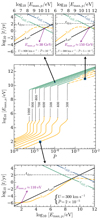Fig. 1. Comparison of timescales and determination of the maximum energy of protons, Emax, p. Central panel: Emax, p versus the shock-accelerated particle pressure, P̃, normalised to the ram pressure for different jet velocities, U, in units of km s−1 (black labels). Solid and dashed orange lines show values of Emax, p constrained by the Coulomb and pion losses, respectively. Solid green lines show Emax, p constrained by the downstream diffusion timescale. Upper and lower panels: timescales involved in the calculation of Emax, p (Eqs. (3)–(7)) for three sets of U and P̃; B = 100 μG, n = 106 cm−3, ℓ⊥ = 400 AU, and R = 12 612 AU.

More specifically, Fig. 1 shows E_max, p as a function of the jet velocity and the cosmic-ray pressure, assuming B = 100 μG, n = 10⁶ cm⁻³, ℓ_⊥ = 400 AU, and R = 12612 AU. It is clearly a threshold process: The central panel of the figure shows that the higher U is, the smaller the fraction of ram pressure that needs to be transferred to thermal particles to jump to the relativistic branch is. This can be understood by noticing that the loss timescale is independent of both U and P̃, while t_acc∝P̃⁻¹U⁻³ (the dynamical and the upstream diffusion timescales are always too long compared to the other timescales and never determine the maximum energy). If P̃ is low (below 4 × 10⁻⁴ and 6 × 10⁻⁶ for U = 300 and 1000 km s⁻¹, respectively), the maximum energy is determined by the intersection of the acceleration and the loss timescales. In this case, Coulomb losses keep E_max, p very low (see the bottom panel) and the acceleration process is inefficient. At larger P̃, depending on U, thermal particles are boosted up to relativistic energies. In this case, E_max, p can be constrained either by pion losses (e.g. U = 300 km s⁻¹ and P̃ > 5 × 10⁻⁴; see the top right panel) or by the downstream diffusion timescale (e.g. U >  700 km s⁻¹; see the top left panel). In fact, for high U, t_acc rapidly decreases, intersecting t_diff, d, and E_max, p increases with increasing P̃ and U since $t_{\mathrm{diff},\mathrm{d}}\propto \stackrel{\sim }{P}U$.

For application to the HOPS 370 jet, the distances, R, of the three synchrotron knots, VLA 12N, 12C, and 12S, from HOPS 370 are about 6955 AU, 10572 AU, and 12612 AU, respectively (Osorio et al. 2017), while the average size of the synchrotron emitting regions is ℓ_⊥ ∼ 400 AU (Tobin et al. 2019). As a consequence, the upstream diffusion timescale never determines the maximum energy since t_diff, u/t_diff, d ≃ 4R/ℓ_⊥ ≫ 1.

2.2. Emerging cosmic-ray energy distribution

The energy distribution per unit density (hereafter distribution) of shock-accelerated protons is given by

$$\begin{array}{c}\hfill {\mathcal{N}}_{\mathrm{p}}(E)=4\pi p^{2}f(p)\frac{\mathrm{d}p}{\mathrm{d}E},\end{array}$$(13)

where f(p) is the momentum distribution at the shock surface. In the test-particle regime, which is valid in this study, this is a power law,

$$\begin{array}{c}\hfill f(p)=f_0{\left(\frac{p}{p_{\mathrm{inj}}}\right)}^{-q},\end{array}$$(14)

with q = 3𝜚/(𝜚 − 1) and p_inj <  p <  p_max, where p_inj is the injection momentum, namely the momentum at which the emerging flux intersects the Maxwellian distribution of thermal particles (see Padovani et al. 2019) and p_max directly derives from E_max, p. The normalisation constant, f₀, is

$$\begin{array}{c}\hfill f_0=\frac{3}{4\pi }\frac{n\stackrel{\sim }{P}}{\mathcal{I}}{\left(\frac{U}{c}\right)}^2{(m_{\mathrm{p}}c)}^{q-3}{p}_{\mathrm{inj}}^{-q},\end{array}$$(15)

where

$$\begin{array}{c}\hfill \mathcal{I}={\displaystyle {\int }_{{\stackrel{\sim }{p}}_{\mathrm{inj}}}^{{\stackrel{\sim }{p}}_{\max }}}\frac{p^{4-q}}{\sqrt{p^2+1}}\mathrm{d}p\end{array}$$(16)

and ${\stackrel{\sim }{p}}_{\mathrm{inj}}$ and ${\stackrel{\sim }{p}}_{\max }$ are the injection and maximum momenta normalised to m_pc (see Padovani et al. 2016).

The electron injection process in shock acceleration is poorly understood. Following Padovani et al. (2019), we adopted the model of Berezhko & Ksenofontov (2000) to estimate the distribution of shock-accelerated electrons, 𝒩_e. Assuming the same energy of the injected electrons as that for protons, namely $p_{\mathrm{inj},\mathrm{e}}=\sqrt{m_{\mathrm{e}}/m_{\mathrm{p}}}{p}_{\mathrm{inj},\mathrm{p}}$ (m_e is the electron mass), at relativistic energies it follows that

$$\begin{array}{c}\hfill \frac{{\mathcal{N}}_{\mathrm{e}}}{{\mathcal{N}}_{\mathrm{p}}}={\left(\frac{m_{\mathrm{e}}}{m_{\mathrm{p}}}\right)}^{(q-3)/2}.\end{array}$$(17)

The electron maximum energy, E_max, e, is limited by synchrotron and inverse Compton losses. However, we checked that, with a local radiation field characterised by an energy density 0.1−10 times that of the interstellar radiation field, as implied by the observed molecular abundance ratios (Karska et al. 2018), inverse Compton losses are at least one order of magnitude smaller than synchrotron losses. Therefore, E_max, e is obtained by equating the acceleration timescale (Eq. (3)) to the synchrotron timescale, t_syn, given by

$$\begin{array}{c}\hfill t_{\mathrm{syn}}=2.7\times {10}^9\frac{\gamma -1}{{\gamma }^2}{\left(\frac{B}{100\mathrm{\mu }\mathrm{G}}\right)}^{-2}\mathrm{yr}.\end{array}$$(18)

If t_syn >  t_acc at any energy, then we set E_max, e = E_max, p. Finally, at energies larger than E^*, where the condition t_syn(E^*)< t_dyn is fulfilled, the slope of the electron distribution, s, is modified from 𝒩_e(E)∝E^s to 𝒩_e(E)∝E^s − 1 (Blumenthal & Gould 1970).

The fluxes for the HOPS 370 jet knots (number of particles per unit energy, time, area, and solid angle) were computed from the corresponding distributions as

$$\begin{array}{c}\hfill j_k=\frac{{\beta }_{k}c}{4\pi }{\mathcal{N}}_k,\end{array}$$(19)

where k = p, e.

2.3. Ionisation rate of locally accelerated particles

Fontani et al. (2017) found an ionisation rate equal to 4 × 10⁻¹⁴ s⁻¹ in a region with an average radius R_ion ∼ 5000 AU towards FIR 4. Since the angular resolution of these observations is 9.5″ × 6.1″, corresponding to 3800 AU × 2440 AU at a distance of ∼400 pc, we assumed that the three radio knots are located at the centre of the region with the enhanced ionisation rate and that each of them contribute one-third of the total ionisation rate. Ionisation by both primary and secondary electrons is negligible, and in the following we only considered the proton component for the calculation of the ionisation rate (see the next section). We computed the propagation of the proton flux at the shock, $j_{\mathrm{p}}^{\mathrm{sh}}$, in each shell of radius r from ℓ_⊥/2 to R_ion, accounting for the attenuation of the flux according to the continuous slowing-down approximation (Padovani et al. 2009). Then, the flux in each shell is given by

$$\begin{array}{c}\hfill j_{\mathrm{p}}(E,r,\delta )=j_{\mathrm{p}}^{\mathrm{sh}}(E_0)\frac{L(E_0)}{L(E)}{\left(\frac{{\ell }_{\perp }/2}{{\ell }_{\perp }/2+r}\right)}^{-\delta }.\end{array}$$(20)

The kinetic energy of a proton decreases from E₀ to E after passing through a column density

$$\begin{array}{c}\hfill N_{\mathrm{r}}=nr=\mathcal{R}(E_0)-\mathcal{R}(E),\end{array}$$(21)

where ℛ is the proton range function defined as

$$\begin{array}{c}\hfill \mathcal{R}(E)={\displaystyle {\int }_0^E}\frac{\mathrm{d}{E}^{\prime }}{L(E^{\prime })}·\end{array}$$(22)

The last factor on the right-hand side of Eq. (20) accounts for the two limiting cases of diffusion (δ = 1; Aharonian 2004) or geometric dilution (δ = 2). Finally, we computed the mean proton flux averaging over the volume of the spherical shell,

$$\begin{array}{c}\hfill ⟨j_{\mathrm{p}}(E,\delta )⟩={\left(\frac{4\pi }{3}{R}_{\mathrm{ion}}^3\right)}^{-1}{\displaystyle {\int }_0^{R_{\mathrm{ion}}}}4\pi r^2{j}_{\mathrm{p}}(E,r,\delta )\mathrm{d}r,\end{array}$$(23)

and the corresponding ionisation rate is

$$\begin{array}{c}\hfill {\zeta }_{\delta }=2\pi {\displaystyle \int ⟨j_{\mathrm{p}}(E,\delta )⟩}{\sigma }_{\mathrm{ion}}(E)\mathrm{d}E,\end{array}$$(24)

where σ_ion is the ionisation cross-section for protons colliding with molecular hydrogen (see e.g. Rudd et al. 1992).

2.4. Synchrotron emission

From the shock-accelerated electron distribution, we computed the expected synchrotron flux density, S_ν, at a frequency ν assuming a Gaussian beam profile and an average size of the synchrotron spots of ℒ_syn ∼ 400 AU (Tobin et al. 2019),

$$\begin{array}{c}\hfill S_{\nu }=\frac{\pi }{4ln2}{ϵ}_{\nu }{\theta }_{\mathrm{b}}^2{\mathcal{L}}_{\mathrm{syn}},\end{array}$$(25)

where θ_b is the beam full size at half maximum and ϵ_ν is the synchrotron specific emissivity,

$$\begin{array}{c}\hfill {ϵ}_{\nu }=\frac{1}{4\pi }{\displaystyle {\int }_{m_{\mathrm{e}}{c}^2}^{\infty }}{\mathcal{N}}_{\mathrm{e}}(E)P_{\nu }^{\mathrm{em}}(E)\mathrm{d}E.\end{array}$$(26)

Here, $P_{\nu }^{\mathrm{em}}(E)$ is the total power per unit frequency emitted at frequency ν by an electron of energy E (see e.g. Longair 2011). We note that we did not account for the attenuation of the electron distribution. In fact, assuming that electrons are created at the centre of a non-thermal knot, they traverse a column density N_syn = nℒ_syn/2 to reach the outer boundary of a knot. Assuming an average volume density of n = 10⁶ cm⁻³, then N_syn = 3 × 10²¹ cm⁻². Therefore, only electrons with energy lower than ∼100 keV are thermalised (see Fig. 2 in Padovani et al. 2018). As a consequence, relativistic electrons responsible for synchrotron emission are not attenuated.

In principle, synchrotron self-absorption could occur at low frequencies when the emitting electrons absorb synchrotron photons (see e.g. Rybicki & Lightman 1986). We computed the optical depth, τ_ν = κ_νℒ_syn, where κ_ν is the absorption coefficient per unit length at frequency ν defined by

$$\begin{array}{c}\hfill {\kappa }_{\nu }=-\frac{c^2}{8\pi {\nu }^2}{\displaystyle {\int }_0^{\infty }}{E}^2\frac{\partial }{\partial E}\left[\frac{{\mathcal{N}}_{\mathrm{e}}(E)}{E^2}\right]P_{\nu }^{\mathrm{em}}(E)\mathrm{d}E,\end{array}$$(27)

and we found that even at the lowest observing frequency (6 GHz), τ_ν ≪ 1; as such, the flux density is straightforwardly determined by Eq. (25).

3. Fitting the model to the synchrotron spectrum

In this section we compare the predictions of our model with the VLA observations of Osorio et al. (2017) for the three non-thermal knots inside the jet generated by HOPS 370, namely VLA 12N, 12C, and 12S. The observations include the C, X, and K bands (at 5 cm, 3 cm, and 1.3 cm, respectively); also included in the fit are the observations in the Ka band (at 9 mm) by Tobin et al. (2019), as anticipated by Osorio et al. (2017). There are five free parameters in our model for synchrotron emission in Eq. (25): the jet velocity in the shock reference frame, U; the fraction of ram pressure transferred to thermal particles, P̃; the magnetic field strength, B; the volume density, n; and the transverse jet width, ℓ_⊥.

Some caveats should be considered before our model is used to interpret the observations. First, due to the lack of information on magnetic field strength and morphology around the shock, we assumed free-streaming propagation to compute the attenuation of the proton flux in each shell (see Eq. (20)). However, since charged particles propagate following a spiral path around magnetic field lines, the traversed effective column density can be much larger, especially if field lines are tangled (Padovani et al. 2013). As a result, the ionisation rate computed with Eq. (24) should be considered as an upper limit. Second, since the energy of the electrons responsible for synchrotron emission is proportional to (ν/B_⊥)^1/2, where B_⊥ is the strength of the magnetic field vector projected on the plane of the sky (e.g. Longair 2011), different parts of the electron distribution are mapped at any given frequency of observation, depending on the local value of B_⊥. Since $P_{\nu }^{\mathrm{em}}$ is also a function of B_⊥, it follows that the specific emissivity (Eq. (26)) spatially depends on the magnetic field. In our model we had to assume a constant value for ϵ_ν along the line of sight, and the flux density computed with Eq. (25) should be regarded as an approximation.

3.1. Bayesian method

We adopted a Bayesian method to infer the best-fit model parameters. Such an approach is particularly helpful in our case because the number of free parameters is commensurate with the number of data points¹. In particular, we used

$$\begin{array}{c}\hfill P(\mathit{\theta }|\mathit{D})\propto P(\mathit{\theta })P(\mathit{D}|\mathit{\theta })\end{array}$$(28)

to derive the full posterior probability distribution, P(θ|D), of the parameter vector θ = (U, P̃, B, n, ℓ_⊥) given the data vector, D (the observed synchrotron spectrum). This posterior is proportional to the product of the prior, P(θ), on all model parameters (the probability of a given model being obtained without knowledge of the data) and the likelihood, P(D|θ), that the data are compatible with a model generated by a particular set of parameters. We assumed that the data are characterised by Gaussian uncertainties, so the likelihood of a given model is proportional to exp(−χ²/2), with

$$\begin{array}{c}\hfill {\chi }^2={\displaystyle \sum _i}{\left(\frac{S_{{\nu }_i}^{\mathrm{obs}}-S_{{\nu }_i}}{{\sigma }_{{\nu }_i}^{\mathrm{obs}}}\right)}^2,\end{array}$$(29)

where $S_{{\nu }_i}^{\mathrm{o}\mathrm{b}\mathrm{s}}$ is the observed flux density at the ith frequency, ν_i; S_νi is the corresponding model flux predicted by Eq. (25); and ${\sigma }_{{\nu }_i}^{\mathrm{o}\mathrm{b}\mathrm{s}}$ is the standard deviation. The best-fit parameter vector, θ, is evaluated by constructing the probability density function (PDF) of a given parameter, weighting each model with the likelihood, and normalising to ensure a total probability of unity. Specifically, this is achieved by marginalisation over other parameters:

$$\begin{array}{c}\hfill P(\mathit{\theta }|\mathit{D})={\displaystyle \int P}(\mathit{\theta },Y|\mathit{D})\mathrm{d}Y,\end{array}$$(30)

where Y is the list of parameters, excluding the parameter of interest.

In our model, the upstream temperature is fixed at the typical value for protostellar shocks of 10⁴ K (Frank et al. 2014), and we assumed a completely ionised medium², x = 1 (Araudo et al. 2007). The chemical model described in Ceccarelli et al. (2014) constrains the density in the range 8 × 10⁵ ≤ n/cm⁻³ ≤ 2 × 10⁶ from the observed abundances of N₂H⁺ and HCO⁺ towards FIR 4. The range of velocity in high-mass protostellar jets is expected to be between 300 and 1000 km s⁻¹ (Marti et al. 1993; Masqué et al. 2012). Since jet velocities are one order of magnitude larger than shock velocities, in the following we assumed that U is equal to the jet velocity. In supernova remnants, the fraction of ram pressure transferred to thermal particles, P̃, is of the order of 10% (Berezhko & Ellison 1999). Since we expect shocks in star-forming regions to be much less energetic, we let $\stackrel{\sim }{P}$ vary between 10⁻⁶ and 10⁻². Finally, for the magnetic field strength, B, we considered a range between 100 μG and the upper limit of ∼10 mG predicted by magnetohydrodynamic jet simulations (Hartigan et al. 2007). The relevant parameter ranges are uniformly sampled, and they are summarised in Table 1. For P̃, B, and n, the parameter space is sampled logarithmically (in 77, 40, and nine intervals, respectively), while for U, the sampling is linear (29 intervals). Although the average size of a knot is ℒ_syn ∼ 400 AU (Tobin et al. 2019), the shock region from which synchrotron emission arises may be smaller. Therefore, we considered four values of ℓ_⊥, namely 100 AU, 200 AU, 300 AU, and 400 AU.

For each of the three VLA knots identified by Osorio et al. (2017), the parameter space of θ was explored through a grid method, stepping through the ranges given by Table 1. However, because of constraints on the ionisation rate driven by accelerated particles, and the requirement of non-zero radio flux densities, the calculation of χ² proceeded in several steps. First, we fixed a pair of velocity and pressure values, (U, P̃), and computed the emerging cosmic-ray flux for every pair of (B, n). From this flux, we then calculated the ionisation rate using all the parameters (U, P̃, B, n) and considered only the pairs (B, n) that gave a ζ(U, P̃, B, n) consistent with the observations (e.g. Fontani et al. 2017). Finally, we required the predicted emerging synchrotron flux to be non-zero. This was accomplished by again examining all pairs of (B, n) and retaining only those parameter configurations of (U, P̃, B, n) that resulted in non-zero synchrotron emission. This exercise resulted in about 8 × 10⁵ different combinations of parameters. For these combinations, we calculated χ² as in Eq. (29) and repeated the procedure for each of the four values of ℓ_⊥.

The size of the emitting region, ℓ_⊥, was sampled somewhat crudely because the model is not particularly sensitive to this parameter; thus, we performed our analysis separately for the four values of ℓ_⊥. Consequently, the marginalisation in Eq. (30) was performed over four parameters, θ = (U, P̃, B, n), and the process was repeated for each value of ℓ_⊥. For each value of ℓ_⊥, we associated the lowest χ² value (the highest likelihood) with the probable best-fit ℓ_⊥. Using only the models with the best-fit ℓ_⊥, determined outside the marginalisation procedure, we took as the best-fit parameter the mode of the PDF, the most probable value in the PDF given by Eq. (30). The best-fit values for U, P̃, B, n, and ℓ_⊥ are reported in Table 1.

3.2. Fitting results

Figure 2 shows corner plots of the best fit obtained for ℓ_⊥ = 100 AU (χ² = 0.09) for VLA 12N. We note that the case ℓ_⊥ = 200 AU is virtually indistinguishable in terms of likelihood. The remaining transverse jet widths for VLA 12N give χ² = 1.36 (300 AU) and 3.84 (400 AU). Figures 3 and 4 show analogous plots for sources VLA 12C and 12S, respectively. For VLA 12C, the best-fit ℓ_⊥ is clearly 100 AU (χ² = 1.36); the other sizes sampled have χ² = 3.81 (200 AU), 8.60 (300 AU), and 13.45 (400 AU). For VLA 12S, the best fit is ℓ_⊥ = 400 AU with χ² = 3.03, even if ℓ_⊥ = 300 AU has χ² = 3.06, confirming that the model is not overly sensitive to size in the broad-brush way we have explored it. The other sizes sampled have χ² = 4.39 (100 AU) and 3.22 (200 AU). These figures also illustrate that some parameters in our model are mutually correlated. In particular, the normalised cosmic-ray pressure, P̃, and the velocity, U, are fairly tightly related, as are P̃ and the magnetic field strength, B. In contrast, none of the parameters seem to depend strongly on the density, n, as shown in the bottom panels of the figures, although this may be a consequence of the relatively narrow range of densities explored in our priors because of the observational constraint given by Ceccarelli et al. (2014). Summaries of the knots are given in the following subsections.

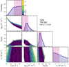Fig. 2. Corner plot of the χ2 surface as a function of the model parameters for VLA 12N. The region size has been fixed externally for these fits. We show an individual corner plot for ℓ⊥ = 100 AU, the best-fit source size. The violet contours correspond to the minimum χ2 value. Top panels in each column: probability density distributions for the marginalised parameters; confidence intervals (±1σ) are shown as violet shaded rectangular regions, and the maximum-likelihood estimate is shown by a vertical dashed line. These values together with the upper and lower uncertainties inferred from the confidence intervals are also reported.

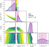Fig. 3. Corner plot of the χ2 surface as a function of the model parameters for the VLA source 12C. The figure is organised as in Fig. 2.

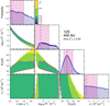Fig. 4. Corner plot of the χ2 surface as a function of the model parameters for the VLA source 12S. The figure is organised as in Fig. 2.

3.2.1. VLA 12N

The jet velocity U is large, but it is not well constrained by our choice of parameters since the best-fit value corresponds to the maximum of the prior, 1000 km s⁻¹. In contrast, both P̃ and B are fairly well determined, both falling towards the lower end of the range of our expectations in the choice of priors. Within the tight range of our priors, the volume density is also somewhat poorly constrained, although within this range the density was fairly well determined independently by Ceccarelli et al. (2014). The best-fit ℓ_⊥ is 100−200 AU, and it can clearly not be as large as 300 AU or 400 AU, at least judging by the significantly larger χ² (corresponding to a likelihood that is four times lower). Overall, the fit to the synchrotron spectrum is exceedingly good, with a very low χ² value, possibly indicating that the errors in the radio fluxes are overestimated.

3.2.2. VLA 12C

The best-fit model parameters are similar to those for source 12N. Although the best-fit B field is nominally larger, the two values are consistent within the errors.

3.2.3. VLA 12S

This source seems to be fundamentally different from the two northernmost ones. The velocity U is about a factor of three lower than in sources 12N or 12C, as if the jet were decelerating due to an impact with a denser medium. This can be explained by noting that the density of the molecular cloud impacted by the termination shock (in our case, 12S) is higher than the density in the jet (see e.g. Torrelles et al. 1986; Rodríguez-Kamenetzky et al. 2017). This causes a deceleration of the jet as well as a decrease in the proper motion velocity of 12S with respect to 12N and 12C as found by Osorio et al. (2017). The 12S proper motion velocity is known, namely its bow shock velocity U_bs = 37 km s⁻¹ (Osorio et al. 2017). Assuming that the velocity we obtain for 12S (U = 350 km s⁻¹) represents the reverse shock velocity, we can then estimate the jet velocity at the termination shock as U + (𝜚−1)U_bs/𝜚 (see e.g. Shore 2007). Since the compression ratio is ∼4 (see Eq. (8)), the jet velocity is 378 km s^{−1 3}. The 12S region itself is also larger, with a size of ℓ_⊥ roughly three or four times that of sources 12N and 12C, revealing a highly collimated jet with an opening angle of ∼1.8°, consistent with the estimate of 2° by Tobin et al. (2019).

4. Comparison with observations

Caution should be taken in interpreting VLA observations with our model. The emissivity is a local quantity that depends on the local electron distribution, 𝒩_e (Eq. (26)). Only with knowing the spatial distribution of both the density and the magnetic field strength is it possible to accurately compute the attenuation of the electron distribution and to rigorously determine the flux density (see e.g. Padovani & Galli 2018). Additionally, for a given B_⊥, the energy of cosmic-ray electrons whose emission peaks at frequency ν is

$$\begin{array}{c}\hfill E_{\mathrm{syn}}\simeq 1.47{\left(\frac{\nu }{\mathrm{GHz}}\right)}^{1/2}{\left(\frac{B_{\perp }}{100\mathrm{\mu }\mathrm{G}}\right)}^{-1/2}\mathrm{GeV}\end{array}$$(31)

(see e.g. Longair 2011). Since the magnetic field strength is not constant, different energy ranges of the electron distribution are sampled when integrating along the line of sight. Due to the uncertainty on the spatial distribution of the model parameters (see Table 1), we are forced to assume constant values. However, for this case study the model has a double constraint, represented by the ionisation rate and the synchrotron emission. This makes the parameter space more restricted. As shown in Fig. 5, in addition to the region where the acceleration process is not efficient in extracting charged particles from the thermal pool (such that no synchrotron radiation is emitted), two big chunks of the space parameters $(U,\stackrel{\sim }{P})$ are ruled out because the range of ionisation rates expected by the model does not include the observed value⁴. The extremes of the range are defined by ζ₁ and ζ₂, the ionisation rates in the case of diffusion and geometrical dilution, respectively (see Eq. (24)). Thus, a solution is found only if the ionisation rate estimated from observations, ζ_obs, falls in the interval [ζ₂, ζ₁]. Putting together the model estimates for the ionisation rate and the non-thermal emission results in a powerful technique for isolating the range of validity for the different parameters.

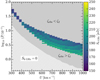Fig. 5. Flux density at 6 GHz obtained with the best-fit procedure for VLA 12C plotted in the space $(\stackrel{\sim }{P},U)$. The hatched area shows where the expected synchrotron emission is null since the acceleration process is inefficient, while the two grey areas show the regions where the constraint given by the ionisation rate estimated by observations, ζobs, is not satisfied, namely ζobs ∉ [ζ2, ζ1].

With this in mind, in Fig. 6 we compare the flux densities observed with those expected by the model. As revealed in advance by the low values of χ², the agreement is particularly good for all three knots. The goodness of fit is a bit poorer for the southern knot since the observation at 8.3 GHz deviates from the clear negative slope traced by the detections at the other four frequencies. The spectral indices for VLA 12N, 12C, and 12S are ${\alpha }_{12\mathrm{N}}=-0.{95}_{-0.02}^{+0.04}$, ${\alpha }_{12\mathrm{C}}=-1.{91}_{-0.01}^{+0.02}$, and ${\alpha }_{12\mathrm{S}}=-0.{36}_{-0.06}^{+0.01}$, respectively, in excellent agreement with those computed by Osorio et al. (2017).

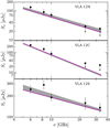Fig. 6. Comparison between the observed flux densities (solid black circles; Osorio et al. 2017; Tobin et al. 2019) and the best-fit models (solid magenta lines) for the three knots, VLA 12N, 12C, and 12S. The grey shaded areas encompass the models within a confidence interval between 50% (second quartile) and 96% (2σ).

5. Discussion and conclusions

In this article we have presented a model showing that cosmic rays accelerated on the surface of a shock, in particular along a protostellar jet, can simultaneously explain the observed molecular abundance (through a high ionisation rate) and the detection of non-thermal emission. Since the latter is generated uniquely by the electronic component of cosmic rays, this allows us to explain the observations without having to rely on shock-generated UV photons.

We have applied the model to the star-forming region OMC-2 FIR 3/FIR 4, the only one in which a likely co-presence of high ionisation and synchrotron radiation has been identified to date. In particular, assuming the interaction between the jet generated by the protostar HOPS 370 within FIR 3 and the FIR 4 protocluster, we were able to indirectly constrain parameters such as the jet velocity, the magnetic field intensity, and the fraction of ram pressure transferred from the shock to the accelerated particles.

By means of Bayesian methods we found high jet velocities for the northern and central knots (650−1000 km s⁻¹ and 750−1000 km s⁻¹, respectively), while in the southern knot U decreases to 300−700 km s⁻¹ as if the jet were hitting a denser medium. The magnetic field strength is well constrained for the three knots between ∼250 μG and ∼450 μG as well as the normalised cosmic-ray pressure between 1.4 and 2 × 10⁻⁵ (even if for VLA 12S the error is quite large). We found transverse widths of the jet between 100 AU (VLA 12N and 12C) and 400 AU (VLA 12S), revealing a highly collimated jet with an opening angle of about 1.8°, consistent with previous estimates (Tobin et al. 2019).

From these quantities, it is also possible to evaluate the intensity of the turbulent magnetic field component, δB, using Eq. (1). For the three knots, VLA 12N, 12C, and 12S, we find B/δB equal to $7_{-5}^{+24}$, ${11}_{-6}^{+22}$, and ${16}_{-14}^{+49}$, respectively, deviating significantly from the Bohm regime (δB ≈ B). From this it follows that the magnetic field should not be completely randomised, unlike in the Bohm regime. Consequently, polarisation observations could help confirm the non-thermal nature of this emission since synchrotron emission is linearly polarised. The fractional polarisation is Π = (3−3α)/(5−3α) (e.g. Longair 2011), and, according to our estimates of the spectral index, Π should be between 67% and 81%. The values obtained with the above relation must be considered as upper limits since this relation is only valid if the magnetic field direction is constant along the line of sight. However, we have shown that the turbulent component of the magnetic field is not negligible, in addition to being fundamental for the efficiency of the acceleration process. This causes the polarisation fraction to decrease. An additional source of depolarisation is represented by the Faraday rotation because of the high electron density at the shock position. This effect is even stronger at lower frequencies (Lee et al. 2019).

Despite the uncertainty regarding the spatial distribution of the fundamental parameters of the model and its relative simplicity, it is evident that the combination of measurements of ionisation rates and synchrotron emission makes it possible to obtain stringent constraints on the physical characteristics of the sources. Beyond the modelling of this single protostellar source, our study aims above all to represent an input for the observers: Observations of co-spatial continuum emission at centimetre wavelengths and molecular transitions can open a new window on the study of star-forming regions. A significant advance in the field is expected in the near future, when a powerful instrument such as the Square Kilometre Array (SKA) will complement facilities already operating at millimetre to metre wavelengths at millimetre and centimetre wavelengths, such as the Atacama Large Millimetre Array (ALMA), NOEMA, the Very Large Array (VLA), the Giant Metrewave Radio Telescope (GMRT), the LOw Frequency ARray (LOFAR), and the Karoo Array Telescope (MeerKAT).

Acknowledgments

We thank the referee for her/his careful reading of the manuscript and insightful comments. M.P. and L.K.H. acknowledge funding from the INAF PRIN-SKA 2017 program 1.05.01.88.04 and by the Italian Ministero dell’Istruzione, Università e Ricerca through the grant Progetti Premiali 2012–iALMA (CUP C52I13000140001). This work has been supported by the project PRIN-INAF-MAIN-STREAM 2017 “Protoplanetary disks seen through the eyes of new-generation instruments”. We also are grateful to Robert Nikutta for enlightening discussions about Bayesian inference.

References

Appendix A: On the adiabatic or radiative nature of the shocks in the HOPS 370 jet

It is usually assumed that the first-order Fermi acceleration mechanism takes place only in the presence of adiabatic shocks. In order to establish the adiabatic or radiative nature of the shocks in the HOPS 370 jet, we applied the criterion described by Blondin et al. (1989). These authors compared the thermal cooling length, d_cool, with the jet half width at the shock position, ℓ_⊥/2. If the ratio of these quantities, λ = d_cool/(ℓ_⊥/2), is much larger than 1, the shock is effectively adiabatic as the shock-heated gas does not have time to cool before leaving the working surface. If λ ≪ 1, the shock is fully radiative⁵. Using the values of the jet velocity in the shock reference frame, the density, and the jet width listed in Table 1, we find that the assumption of adiabaticity is marginally consistent only for the 12N and 12C knots ($\lambda =1.{16}_{-1.04}^{+0.00}$ and $0.{77}_{-0.61}^{+0.26}$, respectively), while 12S is clearly a radiative shock ($\lambda /{10}^{-3}=2.{30}_{-1.55}^{+55.8}$).

However, the common assumption that the first-order Fermi acceleration mechanism cannot occur in radiative collisionless shocks has to be taken with caution for two reasons: (i) radiative shocks can re-accelerate background cosmic rays as well as previously accelerated thermal particles, as is likely the case in evolved supernova remnants (Raymond et al. 2020; ii) recent detections of gamma-ray emission in classical novae by the Fermi telescope also point to the possibility that the first-order Fermi acceleration mechanism takes place in fast radiative shocks, where the acceleration timescale is shorter than any energy-loss timescale, such as that of Coulomb losses, that may quench the acceleration process (Metzger et al. 2015). Therefore, at this stage, it cannot be definitely ruled out that first-order Fermi acceleration also occurs in radiative shocks.

All Tables

All Figures

Fig. 1. Comparison of timescales and determination of the maximum energy of protons, Emax, p. Central panel: Emax, p versus the shock-accelerated particle pressure, P̃, normalised to the ram pressure for different jet velocities, U, in units of km s−1 (black labels). Solid and dashed orange lines show values of Emax, p constrained by the Coulomb and pion losses, respectively. Solid green lines show Emax, p constrained by the downstream diffusion timescale. Upper and lower panels: timescales involved in the calculation of Emax, p (Eqs. (3)–(7)) for three sets of U and P̃; B = 100 μG, n = 106 cm−3, ℓ⊥ = 400 AU, and R = 12 612 AU.

In the text

Fig. 2. Corner plot of the χ2 surface as a function of the model parameters for VLA 12N. The region size has been fixed externally for these fits. We show an individual corner plot for ℓ⊥ = 100 AU, the best-fit source size. The violet contours correspond to the minimum χ2 value. Top panels in each column: probability density distributions for the marginalised parameters; confidence intervals (±1σ) are shown as violet shaded rectangular regions, and the maximum-likelihood estimate is shown by a vertical dashed line. These values together with the upper and lower uncertainties inferred from the confidence intervals are also reported.

In the text

	Fig. 3. Corner plot of the χ2 surface as a function of the model parameters for the VLA source 12C. The figure is organised as in Fig. 2.
In the text

	Fig. 4. Corner plot of the χ2 surface as a function of the model parameters for the VLA source 12S. The figure is organised as in Fig. 2.
In the text

Fig. 5. Flux density at 6 GHz obtained with the best-fit procedure for VLA 12C plotted in the space $(\stackrel{\sim }{P},U)$. The hatched area shows where the expected synchrotron emission is null since the acceleration process is inefficient, while the two grey areas show the regions where the constraint given by the ionisation rate estimated by observations, ζobs, is not satisfied, namely ζobs ∉ [ζ2, ζ1].

In the text

	Fig. 6. Comparison between the observed flux densities (solid black circles; Osorio et al. 2017; Tobin et al. 2019) and the best-fit models (solid magenta lines) for the three knots, VLA 12N, 12C, and 12S. The grey shaded areas encompass the models within a confidence interval between 50% (second quartile) and 96% (2σ).
In the text

References

- Aharonian, F. A. 2004, Very High Energy Cosmic Gamma Radiation: A Crucial Window on the Extreme Universe (World Scientific Publishing) [CrossRef] [Google Scholar]
- Ainsworth, R. E., Scaife, A. M. M., Ray, T. P., et al. 2014, ApJ, 792, L18 [Google Scholar]
- Araudo, A. T., Romero, G. E., Bosch-Ramon, V., & Paredes, J. M. 2007, A&A, 476, 1289 [NASA ADS] [CrossRef] [EDP Sciences] [Google Scholar]
- Bacalla, X. L., Linnartz, H., Cox, N. L. J., et al. 2019, A&A, 622, A31 [EDP Sciences] [Google Scholar]
- Beltrán, M. T., Cesaroni, R., Moscadelli, L., et al. 2016, A&A, 593, A49 [NASA ADS] [CrossRef] [EDP Sciences] [Google Scholar]
- Berezhko, E. G., & Ellison, D. C. 1999, ApJ, 526, 385 [NASA ADS] [CrossRef] [Google Scholar]
- Berezhko, E. G., & Ksenofontov, L. T. 2000, Astron. Lett., 26, 639 [NASA ADS] [CrossRef] [Google Scholar]
- Blondin, J. M., Konigl, A., & Fryxell, B. A. 1989, ApJ, 337, L37 [NASA ADS] [CrossRef] [Google Scholar]
- Blumenthal, G. R., & Gould, R. J. 1970, Rev. Mod. Phys., 42, 237 [NASA ADS] [CrossRef] [Google Scholar]
- Bovino, S., Ferrada-Chamorro, S., Lupi, A., Schleicher, D. R. G., & Caselli, P. 2020, MNRAS, 495, L7 [CrossRef] [Google Scholar]
- Caselli, P., Walmsley, C. M., Terzieva, R., & Herbst, E. 1998, ApJ, 499, 234 [Google Scholar]
- Ceccarelli, C., Dominik, C., López-Sepulcre, A., et al. 2014, ApJ, 790, L1 [NASA ADS] [CrossRef] [Google Scholar]
- Dewangan, L. K., Ojha, D. K., Sharma, S., et al. 2020a, ApJ, 903, 13 [Google Scholar]
- Dewangan, L. K., Sharma, S., Pandey, R., et al. 2020b, ApJ, 898, 172 [Google Scholar]
- Favre, C., Ceccarelli, C., López-Sepulcre, A., et al. 2018, ApJ, 859, 136 [NASA ADS] [CrossRef] [Google Scholar]
- Fontani, F., Ceccarelli, C., Favre, C., et al. 2017, A&A, 605, A57 [NASA ADS] [CrossRef] [EDP Sciences] [Google Scholar]
- Frank, A., Ray, T. P., Cabrit, S., et al. 2014, in Protostars and Planets VI, eds. H. Beuther, R. S. Klessen, C. P. Dullemond, & T. Henning, 451 [Google Scholar]
- Fuente, A., Cernicharo, J., Roueff, E., et al. 2016, A&A, 593, A94 [NASA ADS] [CrossRef] [EDP Sciences] [Google Scholar]
- Furlan, E., Megeath, S. T., Osorio, M., et al. 2014, ApJ, 786, 26 [NASA ADS] [CrossRef] [Google Scholar]
- Furlan, E., Fischer, W. J., Ali, B., et al. 2016, ApJS, 224, 5 [NASA ADS] [CrossRef] [Google Scholar]
- Gaches, B. A. L., & Offner, S. S. R. 2018, ApJ, 861, A87 [Google Scholar]
- Hacar, A., Tafalla, M., Forbrich, J., et al. 2018, A&A, 610, A77 [NASA ADS] [CrossRef] [EDP Sciences] [Google Scholar]
- Hartigan, P., Raymond, J., & Hartmann, L. 1987, ApJ, 316, 323 [NASA ADS] [CrossRef] [Google Scholar]
- Hartigan, P., Frank, A., Varniére, P., & Blackman, E. G. 2007, ApJ, 661, 910 [NASA ADS] [CrossRef] [Google Scholar]
- Heathcote, S., Reipurth, B., & Raga, A. C. 1998, AJ, 116, 1940 [NASA ADS] [CrossRef] [Google Scholar]
- Indriolo, N., & McCall, B. J. 2012, ApJ, 745, 91 [NASA ADS] [CrossRef] [Google Scholar]
- Indriolo, N., Neufeld, D. A., Gerin, M., et al. 2015, ApJ, 800, 40 [NASA ADS] [CrossRef] [Google Scholar]
- Karska, A., Kaufman, M. J., Kristensen, L. E., et al. 2018, ApJS, 235, 30 [Google Scholar]
- Kounkel, M., Hartmann, L., Loinard, L., et al. 2017, ApJ, 834, 142 [Google Scholar]
- Lee, H., Cho, J., & Lazarian, A. 2019, ApJ, 877, 108 [Google Scholar]
- Longair, M. S. 2011, High Energy Astrophysics (Cambridge, UK: Cambridge University Press) [Google Scholar]
- López-Sepulcre, A., Taquet, V., Sánchez-Monge, Á., et al. 2013, A&A, 556, A62 [NASA ADS] [CrossRef] [EDP Sciences] [Google Scholar]
- Maret, S., & Bergin, E. A. 2007, ApJ, 664, 956 [Google Scholar]
- Marti, J., Rodriguez, L. F., & Reipurth, B. 1993, ApJ, 416, 208 [NASA ADS] [CrossRef] [Google Scholar]
- Masqué, J. M., Girart, J. M., Estalella, R., Rodríguez, L. F., & Beltrán, M. T. 2012, ApJ, 758, L10 [NASA ADS] [CrossRef] [Google Scholar]
- Meng, F., Sánchez-Monge, Á., Schilke, P., et al. 2019, A&A, 630, A73 [NASA ADS] [CrossRef] [EDP Sciences] [Google Scholar]
- Metzger, B. D., Finzell, T., Vurm, I., et al. 2015, MNRAS, 450, 2739 [NASA ADS] [CrossRef] [Google Scholar]
- O’C Drury, L., Duffy, P., & Kirk, J. G. 1996, A&A, 309, 1002 [NASA ADS] [Google Scholar]
- Osorio, M., Díaz-Rodríguez, A. K., Anglada, G., et al. 2017, ApJ, 840, 36 [NASA ADS] [CrossRef] [Google Scholar]
- Padovani, M., & Galli, D. 2011, A&A, 530, A109 [NASA ADS] [CrossRef] [EDP Sciences] [Google Scholar]
- Padovani, M., & Galli, D. 2018, A&A, 620, L4 [NASA ADS] [CrossRef] [EDP Sciences] [Google Scholar]
- Padovani, M., Galli, D., & Glassgold, A. E. 2009, A&A, 501, 619 [NASA ADS] [CrossRef] [EDP Sciences] [Google Scholar]
- Padovani, M., Hennebelle, P., & Galli, D. 2013, A&A, 560, A114 [NASA ADS] [CrossRef] [EDP Sciences] [Google Scholar]
- Padovani, M., Hennebelle, P., Marcowith, A., & Ferrière, K. 2015, A&A, 582, L13 [NASA ADS] [CrossRef] [EDP Sciences] [Google Scholar]
- Padovani, M., Marcowith, A., Hennebelle, P., & Ferrière, K. 2016, A&A, 590, A8 [NASA ADS] [CrossRef] [EDP Sciences] [Google Scholar]
- Padovani, M., Ivlev, A. V., Galli, D., & Caselli, P. 2018, A&A, 614, A111 [NASA ADS] [CrossRef] [EDP Sciences] [Google Scholar]
- Padovani, M., Marcowith, A., Sánchez-Monge, Á., Meng, F., & Schilke, P. 2019, A&A, 630, A72 [NASA ADS] [CrossRef] [EDP Sciences] [Google Scholar]
- Padovani, M., Ivlev, A. V., Galli, D., et al. 2020, Space Sci. Rev., 216, 29 [Google Scholar]
- Parizot, E., Marcowith, A., Ballet, J., & Gallant, Y. A. 2006, A&A, 453, 387 [NASA ADS] [CrossRef] [EDP Sciences] [Google Scholar]
- Pelletier, G., Lemoine, M., & Marcowith, A. 2006, A&A, 453, 181 [NASA ADS] [CrossRef] [EDP Sciences] [Google Scholar]
- Podio, L., Lefloch, B., Ceccarelli, C., Codella, C., & Bachiller, R. 2014, A&A, 565, A64 [NASA ADS] [CrossRef] [EDP Sciences] [Google Scholar]
- Porras, A. J., Federman, S. R., Welty, D. E., & Ritchey, A. M. 2014, ApJ, 781, L8 [NASA ADS] [CrossRef] [Google Scholar]
- Raymond, J. C., Chilingarian, I. V., Blair, W. P., et al. 2020, ApJ, 894, 108 [CrossRef] [Google Scholar]
- Rodríguez-Kamenetzky, A., Carrasco-González, C., Araudo, A., et al. 2017, ApJ, 851, 16 [NASA ADS] [CrossRef] [Google Scholar]
- Rudd, M. E., Kim, Y. K., Madison, D. H., & Gay, T. J. 1992, Rev. Mod. Phys., 64, 441 [NASA ADS] [CrossRef] [Google Scholar]
- Rybicki, G. B., & Lightman, A. P. 1986, Radiative Processes in Astrophysics (Wiley-VCH), 400 [Google Scholar]
- Sabatini, G., Bovino, S., Giannetti, A., et al. 2020, A&A, 644, A34 [EDP Sciences] [Google Scholar]
- Sanna, A., Moscadelli, L., Goddi, C., et al. 2019, A&A, 623, L3 [NASA ADS] [CrossRef] [EDP Sciences] [Google Scholar]
- Shalchi, A. 2009, Nonlinear Cosmic Ray Diffusion Theories (Berlin, Heidelberg: Springer-Verlag), 362 [CrossRef] [Google Scholar]
- Shimajiri, Y., Takahashi, S., Takakuwa, S., Saito, M., & Kawabe, R. 2008, ApJ, 683, 255 [NASA ADS] [CrossRef] [Google Scholar]
- Shore, S. N. 2007, Astrophysical Hydrodynamics: An Introduction (Weinheim: Wiley) [CrossRef] [Google Scholar]
- Silsbee, K., Ivlev, A. V., Padovani, M., & Caselli, P. 2018, ApJ, 863, 188 [CrossRef] [Google Scholar]
- Tobin, J. J., Megeath, S. T., van’t Hoff, M., et al. 2019, ApJ, 886, 6 [Google Scholar]
- Torrelles, J. M., Ho, P. T. P., Moran, J. M., Rodriguez, L. F., & Canto, J. 1986, ApJ, 307, 787 [NASA ADS] [CrossRef] [Google Scholar]
- Zhao, D., Galazutdinov, G. A., Linnartz, H., & Krełowski, J. 2015, ApJ, 805, L12 [NASA ADS] [CrossRef] [Google Scholar]