| Issue |
A&A
Volume 648, April 2021
|
|
|---|---|---|
| Article Number | A79 | |
| Number of page(s) | 9 | |
| Section | Stellar atmospheres | |
| DOI | https://doi.org/10.1051/0004-6361/202040148 | |
| Published online | 15 April 2021 | |
Stochastic light variations in hot stars from wind instability: finding photometric signatures and testing against the TESS data
1
Department of Theoretical Physics and Astrophysics, Faculty of Science, Masaryk University,
Kotlářská 2,
Brno,
Czech Republic
e-mail: krticka@physics.muni.cz
2
Institut für Physik und Astronomie, Universität Potsdam, Karl-Liebknecht-Straße 24/25,
Potsdam-Golm,
Germany
Received:
16
December
2020
Accepted:
1
March
2021
Context. Line-driven wind instability is expected to cause small-scale wind inhomogeneities, X-ray emission, and wind line profile variability. The instability can already develop around the sonic point if it is initiated close to the photosphere due to stochastic turbulent motions. In such cases, it may leave its imprint on the light curve as a result of wind blanketing.
Aims. We study the photometric signatures of the line-driven wind instability.
Methods. We used line-driven wind instability simulations to determine the wind variability close to the star. We applied two types of boundary perturbations: a sinusoidal one that enables us to study in detail the development of the instability and a stochastic one given by a Langevin process that provides a more realistic boundary perturbation. We estimated the photometric variability from the resulting mass-flux variations. The variability was simulated assuming that the wind consists of a large number of independent conical wind sectors. We compared the simulated light curves with TESS light curves of OB stars that show stochastic variability.
Results. We find two typical signatures of line-driven wind instability in photometric data: a knee in the power spectrum of magnitude fluctuations, which appears due to engulfment of small-scale structure by larger structures, and a negative skewness of the distribution of fluctuations, which is the result of spatial dominance of rarefied regions. These features endure even when combining the light curves from independent wind sectors.
Conclusions. The stochastic photometric variability of OB stars bears certain signatures of the line-driven wind instability. The distribution function of observed photometric data shows negative skewness and the power spectra of a fraction of light curves exhibit a knee. This can be explained as a result of the line-driven wind instability triggered by stochastic base perturbations.
Key words: stars: winds, outflows / stars: mass-loss / stars: early-type / hydrodynamics / instabilities / stars: variables: general
© ESO 2021
1 Introduction
The stellar winds of hot stars are mostly driven by radiative acceleration in the lines of such elements as carbon, oxygen, silicon, and iron (Lucy & Solomon 1970; Castor et al. 1975). This acceleration is inherently unstable. Due to the Doppler effect, small positive perturbations of the velocity displace the lines from their equilibrium positions and expose the line to unabsorbed stellar flux, which leads to a substantial increase in the radiative force (MacGregor et al. 1979; Carlberg 1980; Owocki & Rybicki 1984).
The perturbations from the line-driven wind instability steepen into reverse shocks (Owocki et al. 1988), providing an explanation for the generic X-ray emission observed in hot stars (Feldmeier et al. 1997). In addition, the instability may magnify the atmospheric density perturbations that exist due to subsurface convection or stellar oscillations (Cantiello et al. 2009; Aerts et al. 2009; Jiang et al. 2015), leading to a complex wind structure typically referred to as clumping. Therefore, one single process may, in fact, connect the photospheric line profile variations (Kholtygin et al. 2011; Martins et al. 2015; Aerts & Rogers 2015), macroturbulent broadening (Dufton et al. 2006; Markova & Puls 2008), and wind variability.
Temporal variability on the part of the wind mass-flux is another consequence of the line-driven wind instability. This contributes to photometric variations of hot stars attributed to a process called wind blanketing. Wind blanketing refers to the absorption of photospheric radiation by the wind and its partial reemission back into the stellar photosphere (Abbott & Hummer 1985). As the atmosphere becomes more opaque, the temperature gradient steepens to transfer the same flux through the opaque region. Effectively, this leads to the heating of the photosphere. Therefore, the inclusion of wind blanketing is important for the determination of atmospheric properties of hot stars with winds (Bohannan et al. 1986; Crowther et al. 2002; Martins et al. 2005). With the increasing opacity, photons progressively escape into spectral regions where the gas is more transparent, which leads to flux redistribution. Therefore, as a result of wind blanketing, a small fraction of the radiative flux emitted by hot stars is absorbed by their winds and redistributed towards longer wavelengths. The amount of redistributed flux depends on the mass-loss rate. Consequently, any process that causes either a temporal or lateral variability of the wind in the regions just above the hydrostatic photosphere also inevitably leads to photometric variability. There are several such effects that can cause wind variability, including magnetic fields (ud-Doula & Owocki 2002), bright surface spots (David-Uraz et al. 2017), and line-driven instability (Owocki et al. 1988; Feldmeier et al. 1997).
Krtička & Feldmeier (2018) used the dependence of the redistributed flux on the mass-loss rate from global wind models (Krtička 2016) and the instability simulations of Feldmeier et al. (1997) to predict the light variability of hot stars. They showed that the combined effects of wind blanketing and instability lead to a stochastic light variability with amplitude on the order of millimagnitudes.
This effect can be compared to the stochastic variability observed in hot stars. Stochastic variability has a relatively low amplitude and although, in some cases, it can be observed from the ground (e.g. Kourniotis et al. 2014), for most stars, precise satellite photometry is required for it to be detected (Blomme et al. 2011; Ramiaramanantsoa et al. 2018; Simón-Díaz et al. 2018). Typically, stochastic variability is attributed to surface oscillations driven by convective motions (Aerts & Rogers 2015; Aerts et al. 2017; Lecoanet et al. 2019).
In the present paper, we use the approach of Feldmeier & Thomas (2017) to better understand the signature of perturbations in the photometry and its dependence on the inner boundary conditions. We study the dependence of the light variability at the height where the optical flux originates and we determine the photometric signatures of the line-driven wind instability.
2 Line-driven wind instability simulations
A consistent treatment of the wind blanketing variability due to the line-driven wind instability is a formidable problem. A suitable approach would require coupling 3D radiative hydrodynamic simulations with a detailed solution of the radiative transfer equation and the determination of nonequilibrium level populations. To make the problem tractable, we split it into two parts: the simulation of the line-driven wind instability and subsequent calculation of light variability based on these hydrodynamic simulations. Our calculations are done in 1D and we construct 3D wind models by dividing the visible stellar surface into patches and integrating over the whole surface under the assumption that individual patches are independent.
2.1 Hydrodynamic equations and their solution
The present level of sophistication of time-dependent numerical wind simulations including the line-driven instability (LDI) is defined in the following papers: Owocki & Puls (1996, 1999), introducing a nonlocal escape-integral source function (EISF) for the scattered radiation field; Sundqvist & Owocki (2015), demonstrating the transition of the solution topology near the sonic point from X-type to nodal type in dependence on the strength of the diffuse radiation field and the ratio of thermal-to-sound speed; and Sundqvist et al. (2018), performing two-dimensional planar simulations of the LDI with the smooth source function (SSF) approach of Owocki (1991) for the scattered radiation field.
The present paper takes a complementary approach and calculates the radiative line force in the simplest possible setting that still shows the LDI, with force-per-mass given by
 (1)
(1)
Here, z is a planar coordinate pointing away from the star, f(z) a function that controls the stationary wind velocity law (and absorbs the Castor et al. (1975, hereafter CAK) line force parameter k), u(z) is the wind velocity law normalised to the thermal speed, vth (assumed to be constant), ϱ(z) is the wind density stratification, x is the normalised frequency displacement from line center in a resonance line with Doppler line profile ϕ(x), and 0 < c ≪ 1 is a cutoff parameter that prevents the wind from becoming completely transparent; the argument of the square-root in the denominator of Eq. (1) is the optical depth in a line with normalised and constant mass absorption coefficient, κ = 1, and the square-root corresponds to the second CAK force parameter α being set to α = 1∕2 (with this value chosen for computational convenience). The line force (1) results from an integration over a power-law distribution in frequency and mass absorption coefficient, N(ν, κ) ~ ν−1κ−3∕2. There is no angle integration in Eq. (1), thus, it is in a single-ray approximation.
We fix the function f(z) so that the resulting wind velocity law is linear, v ~ z. The reason for this is that the steepness of the CAK velocity law near the sonic point causes a very swift length-stretching of the perturbations. The initial growth of the LDI structure cannot be followed in sufficient detail thus, and nonlinear effects appear to occur quite suddenly. Nonlinear effects include the excitation of a large number of harmonic overtones of the perturbation and the mutual collisions and coalescence of density enhancements (shell-shell-collisions); for more, see Feldmeier (1995). By assuming u(z) ~ z, the wind structure grows in arithmetic (velocity) and geometric (density) progression as function of z and all steps of its evolution can be followed in detail.
This description of the line force shows the pure LDI without any intervening or competing effects. Since we also neglect thermal gas pressure and gravity, and since the radiative force in Eq. (1) depends on the windvelocity and density alone, there is thus a kinematical model for the wind and the LDI (if allowing for inertial mass in kinematics). Since the Sobolev approximation has the velocity gradient entering grad in Eq. (1) via  , the force in Eq. (1) still leads to an eigenvalue problem for the mass-loss rate in the Euler equation with an X-type CAK critical point (not the sonic point) that separates shallow (‘breeze’) solutions from steep (‘overloaded’ or ‘failed’) ones.
The structure developing from the unstable growth of perturbations introduced at a rather large amplitude at the inner boundary is at a maximum since scattering is left out intentionally, thus there is no stabilising line drag effect (Lucy 1984). Furthermore, no Schuster-Schwarzschild absorbing layer is used to reduce the radiative flux at small speeds on the order a few vth (see again Owocki et al. 1988). Finally, the sound speed and the gravity are set to zero. Thus, there is no barometric density stratification at the inner boundary and the line force is the only force present (apart from numerical viscosity). The effects of these simplifications are discussed in Sect. 5.
We performed hydrodynamic simulations using the code developed by Feldmeier & Thomas (2017). The code solves the Euler and continuity equations for a wind subject to the line-driven instability from a pure absorption line force in planar geometry. We use a simple time-explicit Euler scheme, where the density, ρ, and the momentum density, ρu, are derived from the continuity and momentum equations solved in integral form. The fluxes at cell boundaries are interpolated from their values inside the cells using the van Leer derivative (van Leer 1977) and consistent advection (Norman et al. 1980; Stone & Norman 1992).
The specific parameters and normalisations of our model are as follows. We emphasise that given the simplicity of Eq. (1), the wind structure is generic, so any reference to a single, real star would be putative and we can only refer to a ‘generic’ O supergiant with a strong wind, for instance, ζ Pup or ζ Ori.
Velocities are given in units of vth. The latter enters the (finite) thermal width of the line profile, which is the most important factor for obtaining the LDI. Distance is normalised such that the velocity law is not only linear, but u(z) = z. Mass units are fixed by assuming a mass flux ϱu = 1 for the stationary wind. With z, u, and m, all units of our (extended) kinematics are fixed (time t = z∕u). As the inner boundary, we assume z = 1∕3 and u = 1∕3, that is, one third of vth. Since the sound speed in hot-star winds is typically a few vth, the inner boundary corresponds to (roughly) 10% the sound speed. The sonic point should be around z = u ≈ 3. We sample the wind structure in the following figures at z = 1 and z = 5.
We use 1000 spatial mesh points with Δz∕z = const. (logarithmic spacing). The Doppler profile of the exemplaric spectral line is resolved by three frequency points per thermal width and 2 × 3 × 3 = 18 points in total.
As the opacity cutoff, we use c = 10−4, which is close to the value used in most simulations thus far. The cutoff serves to avoid steep acceleration of highly rarefied intershell gas. In Feldmeier & Thomas (2017), we also used c = 10−10, showing thissteep acceleration, but with essentially no difference for the gas at the moderate densities that we are interested here.
At the inner boundary, we assume perturbations in the mass flux ϱu but keep the density ϱ fixed. We implemented two types of inner boundary perturbations, sinusoidal and Langevin perturbations. The former can help us to understand the development of wind structure and the latter provides a more realistic model for atmospheric perturbations, which are likely to be the result of subsurface convection and which contain many pulsational modes. We chose a perturbation period and correlation period that are roughly equal to the wind flow time and atmospheric cutoff period, which corresponds to the values given in Feldmeier et al. (1997).
2.2 Results of hydrodynamic simulations
Figure 1 shows snapshots of hydrodynamic simulations for sinusoidal and Langevin base perturbations. The instability fully develops at a velocity of several thermal speeds, leading to strong overdensities moving roughly at the speed of the unperturbed wind. The rarefied matter between dense clumps is strongly accelerated and accumulates in the closest overdensity at larger height. Compared to sinusoidal base perturbations, the Langevin base perturbation leads to a less regular structure of overdensities.
We studied wind variations close to the star where the light variability originates. For small base perturbations, the instability fully develops only at very large velocities and, consequently, it does not cause large mass-loss rate variations close to the photosphere. On the other hand, for large base perturbations, the line-driven wind significantly affects the wind structure already at velocities close to the thermal speed (see Fig. 2). The amplitude of the boundary perturbation should be on the order of 0.3–0.5 thermal speeds to cause significant variability at a low height.
The model with sinusoidal base perturbations (Fig. 2, upper panel) shows the connection between boundary conditions and the development of wind structure. Close to the boundary, the variations of the mass flux still resemble the boundary perturbations. As the line-driven instability develops, the maximum perturbations steepen into shocks collecting inner low-density material moving at high speed.
This also provides the basic explanation of the structure shown for Langevin boundary perturbations in Fig. 2 (bottom panel). At high velocities, only the largest overdensities prevail, originating from the largest surface perturbations and engulfed subsequent smaller perturbations.
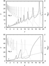 |
Fig. 1 Snapshot of height variations of the wind velocity (black lines) and density (gray lines) compared with the stationary CAK solution (dashed lines), plotted for sinusoidal base perturbation (upper panel) and for the Langevin base perturbation (lower panel). Calculations are performed in non-dimensional units with velocity expressed in units of the thermal speed. |
3 Modelling the light variability
3.1 Integrating over the stellar disk: single surface patch
The predicted time variability of the mass flux is used to derive light variations and light curves. We used the formula from Krtička (2016), based on the global spherically symmetric METUJE wind models and described by Krtička & Kubát (2017), which connects the mass flux variations ρu at a given height with photometric variability:
 (2)
(2)
Here, the fit parameter, ΔF = 1.6 × 10⁷ erg s−1 cm−2, describes the strength of the wind blanketing effect; F0 = 9.0 × 10⁸ erg s−1 cm−2 is the emergent flux for a reference mass-loss rate; and ⟨ρu⟩ is the mean mass flux. This relation was derived for a typical O star with parameters corresponding to HD 191612.
We calculated the light curves for both types of base perturbations (sinusoidal and Langevin turbulence) and for mass flux variations at different heights (see Fig. 3). These variations closely follow the mass flux variations in Fig. 2. For large boundary perturbations, the instability develops sharp density peaks already in the subsonic part of the wind. These peaks also appear in the mass-loss rate variations and, consequently, also in photometric variations due to wind blanketing. Because the peaks of the density variations are not fully symmetric, the derived light variation becomes also slightly asymmetric. Predicted sharp brightness peaks are typical for the light variability of O stars connected with the line-driven wind instability and can, therefore, provide an observational test of the appearance of the instability.
Another signature of the line-driven wind instability is seen in the distribution of magnitude differences in Fig. 4. The distribution at the base of the wind given by the boundary conditions is significantly modified by the line-driven instability. Not only does the distribution become wider, but its shape is modified as well. From Fig. 4, it follows that the peak shifts to positive magnitude differences, while the tail formed by the brightness maxima is more extended. This originates due to the structure generated by the line-driven wind instability with sharp overdensity regions where the sharp brightness maxima form, followed by broad underdensity regions where the broad photometric minima have their origin.
This is also seen in the value of the skewness introduced as  , where x is variable, the overline denotes mean value, and s is the sample standard deviation. The skewness becomes negative for large velocities (γ1 = −0.27 at u = 5 for Langevin perturbations). Negative skewness implies that the magnitude distribution has a tail on its brighter side, which is formed during the short period when the overdensities appear, while most of the values appear on the dimmer side of the distribution originating in the thin gas.
From the time-frequency analysis, it follows that the frequency spectrum is more or less constant with time. On the other hand, the perturbations evolve as they move in the wind. The radial development of instability structure can be seen in the power spectrum of light variations in Fig. 5. While the perturbations close to the base are given by a uniform power law due to the Langevin perturbations, the variability at large heights shows a more complex, broken power law. As the high-frequency perturbations with low density move faster, they collide and merge with less frequent high-density perturbation. Consequently, the line-driving filters out power at higher frequencies and maintains large low-frequency perturbations.
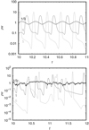 |
Fig. 2 Variability of the mass flux at u = 1∕3, u = 1, and u = 5 (increasing amplitude) for sinusoidal (upper panel) and Langevin base perturbations (lower panel). Calculations are performed in nondimensional units with stationary mass flux ρu = 1. |
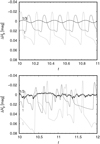 |
Fig. 3 Light variability for sound wave (upper panel) and Langevin boundary perturbations (bottom panel). Individual curves are calculated from the mass flux variations for velocities u = 1∕3, u = 1, and u = 5. The graph shows the difference between actual magnitude and magnitude predicted for the mean flux. |
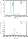 |
Fig. 4 Histograms of the distribution of magnitude differences for sound wave perturbations (upper panel) and Langevin perturbations (bottom panel), for u = 1∕3, 1, and 5. The ordinate gives the relative frequency divided by the box width, i.e, the distribution function. It is normalised in such a way that its integral over all magnitude differences is unity. |
 |
Fig. 5 Power spectrum of light variability for Langevin base perturbations, for velocities u = 1∕3 and u = 5. Determined as a magnitude of the coefficients of the Fourier transform of the light curves. |
3.2 Integrating over the stellar disk: multiple surface patches
So far, we have assumed that the stellar surface consists of a single patch and that the wind structure does not depend on the lateral coordinates. This is a very artificial assumption and we would expect that the boundary perturbations triggering the line-driven instability are not coherent across the stellar surface.
To account for the lateral fragmentation of the wind structure, we follow the approach of Dessart & Owocki (2002) and Feldmeier et al. (2003), dividing the stellar wind into N concentric spherical cones and assuming that the wind structure in each of these cones is independent from neighboring cones. The mass flux at the time, t, in each coneis derived by randomly shifting the simulated mass flux over time:
 (3)
(3)
where the index i counts the cones, Ωi is the solid angle subtended by a cone, and Δti is a random variable. We assume that Δti has a uniform distribution over the simulation time, ΔT, and that the mass flux varies periodically with the same period ΔT. We selected the cones in such a way that the solid angle Ωi is roughly the same for each one and integrate the flux from all cones across the visible surface (see Krtička & Feldmeier 2018 for details). For the integration, we adopt the limb darkening coefficients from Reeve & Howarth (2016).
Hydrodynamic simulations predict a typical lateral scale of structure generated by the line-driven instability of about 0.01 R* (Sundqvist et al. 2018). This corresponds to a patch size for wind structure on the order of several degrees, as also inferred from emission line profile variability by Dessart & Owocki (2002). A small lateral size for the wind structure is also consistent with the number of clumps in the observable part of the wind, which is on the order of 103 –105, as estimated from the observed level of polarimetric variability (Davies et al. 2007), from the strength of wind line profiles (Oskinova et al. 2007; Šurlan et al. 2013), and from the level of short-term X-ray variability (Nazé et al. 2013). Therefore, we selected N = 300 and N = 103 for the following simulations.
Obviously, as a result of summing over independent light curves, the amplitude of the variability decreases with increasing N (Krtička &Feldmeier 2018). However, the variability remains detectable even for a relatively large number of cones, N = 103 (Fig. 6). The form of the boundary perturbation has a significant influence even on the combined light curves as the light curve for sound wave boundary perturbations retains some kind of quasi-periodicity.
After summing up over the independent cones, the distribution of magnitude differences approaches a normal distribution (Fig. 7). Still, even for a large number of patches on the order of hundreds, the distribution resulting from the Langevin base perturbation shows negative skewness. This indicates that the magnitude distribution function has an extended tail on its brighter side. We derived γ1 = −0.030 for N = 300 and γ1 = −0.015 for N = 103 at u = 5 and by averaging over 103 random realisations of light curves. This means that periods of lower flux (positive magnitude difference) formed in underdensities are more frequent than periods of higher flux (negative magnitude difference) formed in overdensities.
The combination of light curves from individual patches also influences the power spectrum of light variations significantly. The power spectrum of the light curve derived from a single patch model shows a characteristic ‘knee’ as a result of the merging of weak small-scale perturbations with large-scale perturbations (Fig. 5). This also occurs when the light curve is combined from several independent cones (Fig. 8).
Finally, we briefly discuss the dependence of light variability on stellar parameters. The height of continuum formation depends on the mass-loss rate. With a rising mass-loss rate, the continuum formation region moves to the upper layers of the atmosphere.Because the instability generated structure strengthens with increasing height, we expect stronger stochastic variability in stars with higher mass-loss rates.
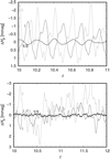 |
Fig. 6 Light variability for sound wave perturbations (upper panel) and Langevin perturbations (bottom panel) summed over N = 103 independent cones, calculated from mass flux variations for u = 1∕3, 1, and 5. The graph shows the difference between actual magnitude and mean. |
4 Testing against the TESS data
We tested the basic predictions of our model against the Transiting Exoplanet Survey Satellite (TESS) data (Ricker et al. 2015). Using the MAST1 web page, we searched for TESS photometric data for O stars contained in the Galactic O-Star Catalog (Maíz Apellániz et al. 2013). We supplemented this list with B supergiants given in Crowther et al. (2006), Lefever et al. (2007), Benaglia et al. (2007), Markova & Puls (2008), and Haucke et al. (2018). The search performed on September 17th 2020 resulted in 216 cross-matched light curves of O stars and 70 of B supergiants, for which we downloaded the light curves observed at a two-minute cadence. The visual inspection of the data showed that all selected stars show some kind of light variability, which is either periodic (that is, mostly due to binary effects or pulsations), or stochastic, or a combination of both (Pedersen et al. 2019; Burssens et al. 2020; Bowman et al. 2020). We selected only stars with purely stochastic variability. We discarded stars having periodical structures in their light curves, which can be attributed to binarity and pulsations, as well as stars whose timescale of variability is comparable to the duration of TESS observations. These effects especially appear in B supergiants, which have larger radii than O stars with the same luminosity. This reduced the list to 116 light curves of O stars and 18 of B supergiants, for which we performed a detailed analysis.
Detailed analyses of the light curves show that the skewness of the distribution function of magnitude differences is non-zero in most stars and it appears to be independent of the stellar parameters. The light curves of most stars have a negative skewness, indicating that dimmer phases prevail slightly and that the distribution has an extended tail on its bright side. A significant fraction of stars show positive skewness and, therefore, the opposite behavior, but the TESS light curves are rather short and the positive skewness may be just a result of random selection of part of the light curve. We plotted the histogram of all magnitude differences relative to dispersion (Fig. 9). The final distribution has a negative skewness of γ1 = −0.084 ± 0.002, corresponding to the mean skewness of all light curves. This agrees with the light variations due to the line-driven wind instability and a wind blanketing that is triggered by Langevin base perturbations averaged over hundreds of independent surface patches.
All simulations of the line-driven instability so far show a sequence of highly overdense and narrow shells or clumps, formed by the accumulation of gas from broad and, as a result, highly rarefied regions between the shells or clumps. This asymmetric density distribution reflects itself in an asymmetric distribution of the visible stellar brightness via blanketing.
Therefore, the detected skewness of the stochastic light curves of OB stars offer direct evidence of a structure generated by line-driven wind instability that already appears close to the photosphere. Within our model, the negative skewness of the light curves is caused by short periods when the light curve is dominated by instability generated large overdensities that lead to brightening of the star in the optical region (negative magnitude difference). These brief periods of maximum light are followed by long periods of light minimum due to rarefied wind regions that follow each overdensity.
The power spectra of light curves of a significant fraction of stars are broken power laws (see Fig. 10). Such power laws with a knee are expected from our simulations as a result of the radial evolution of base perturbations, during which small-scale perturbations are engulfed by large-scale perturbations. Consequently, this feature can be also attributed to the line-driven wind instability.
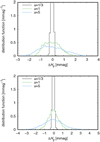 |
Fig. 7 Histogram of the distribution of magnitude differences for sound wave perturbations (upper panel) and Langevin perturbations (bottom panel) summed over N = 103 independent cones, calculated from mass flux variations at u = 1∕3, 1, and 5. |
 |
Fig. 8 Power spectrum derived from the light curve summed over N = 300 and N =103 independent cones (given in Fig. 6) for the case of Langevin base perturbation at velocity u = 5. |
 |
Fig. 9 Distribution of flux variations of TESS observations |
5 Discussion
An advantage of the reduced description of the line force and wind hydrodynamics introduced in Sect. 2.1 is that it givesthe ‘pure’ LDI and thus a clear picture of the generic structure that develops from the maximum possible radiation force (no backscattering). This structure is highly non-linear, with shock fronts of Mach number ≤ 30 (it is questionable, however, how meaningful a reference of radiative shock strength to thermal gas pressure realy is). Still, gas pressure and radiative scattering, which is neglected in the present work, can have severe influence on the wind dynamics. Here, we discuss a few of these effects.
Firstly, the so-called line-drag effect of Lucy (1984) causes a partial compensation of the LDI by backscattered photons. In the extreme case that half the photons are backscattered, as may happen near the star, the LDI has completely vanished. When using the SSF force in our simulations (not shown in the present paper) with a backscattering fraction of 1/2 throughout the wind, we obtain a wind that is completely stable, base perturbations are not amplified, and the wind stays near its stationary solution; there is thus no LDI structure at all. Therefore, any quantitative estimate for the strength of wind structure must include line scattering.
Secondly, by including thermal pressure and gravity, the wind velocity grows exponentially up to the sonic point, then switches to the CAK wind velocity law (the latter having an infinite slope at r = R*). This transition between different velocity laws is accompanied by large changes in the velocity gradient, u′, which leads to fore-aft asymmetries in the escape probabilities (the larger u′, the lower is the Sobolev optical depth in the line). The importance of this shows up most prominently in the EISF formulation of the radiative force, with a source function S = βc∕β, where β is the escape probability in any direction, βc is the same but for directions towards the stellar disk, and where β and βc are calculated from the actual, time-dependent wind structure, thus allowing for another feedback (apart from that of the optical depth on the line force as in Eq. (1)) of the hydrodynamics on the radiation field. Owocki & Puls (1999) find that a depression in the source function near the sonic point alters the mean wind conditions. The EISF models settle to the unique steep solution of a nodal-type critical point. Sundqvist & Owocki (2015) find that with S → 0, the solution topology near the sonic point changes from X-type (as in CAK) to nodal type, the latter having a steep branch through which a unique solution passes and a shallow branch with a ‘degenerate’ family of solutions (all with the same u′).
Thirdly, this nodal solution topology at the sonic point was already found by Poe et al. (1990) for a pure absorption line model. They find that at vth∕a = 1∕2, the wind settles in the unique steep branch at the node and the overall velocity law appears to be too fast; whereas for realistic values, vth ∕a = 1∕3, the wind favors the lower node branch that has a whole solution family. Their degeneracy causes intrinsic, self-excited wind variability with the wind sampling through all possible solutions.
Next, by including thermal pressure, perturbations grow exponentially in the subsonic wind region already without any radiative force (by pure energy conservation of a sound wave in a barometric stratification), eventually leading to so-called shock levitation in dust-driven winds from cool stars. Sound waves then travel forth and back through the wind between the inner boundary and the sonic point. This has some poorly understood influence on the stability of the inner wind. Current simulations have to adopt therefore a photospheric speed of roughly 10% the sound speed. Using 1 or 30% instead, the simulations show huge oscillations and usually crash.
Therefore, both the pure absorption model and the models including scattering (SSF and EISF) show complications at the critical point, with transitions from X-type to nodal type solution topology, and with possible consequences for the overall wind dynamics (a stable steep solution versus a degenerate, self-excited shallow solution). In contrast, our pure absorption models without thermal gas pressure that are presented here show no peculiarities. Without explicit perturbations at the wind base, the wind remains perfectly stable for the u = z solution. With a periodic base perturbation, the unstable structure from the line force in Eq. (1) gives a temporally well-resolved and uniform growth of unstable structure from linear to highly nonlinear phases. Since we are interested in the velocity law at small distances from the star near the sonic point, this conditioning of the velocity law u(z) to u(z) = z should have no significant influence on our results, but this makes the numerics much more robust compared to calculations including thermal pressure and scattering.
The resulting structure is the one that was first described by Owocki et al. (1988) and Owocki (1991): the LDI enhances positive perturbations of u′ and accelerates corresponding material until it is eventually decelerated by the gas preceding it, which has either no or negative velocity-gradient perturbations and thus remains at the stationary CAK wind speed. The deceleration of gas happens in a strong reverse shock with huge density contrasts (assuming there are no thermal energy losses, i.e. there is no gas heating). We note in passing thatearlier simulations of the pure absorption line force encountered certain difficulties caused by the very strength of the LDI, which were overcome, for instance, by a Schuster-Schwarzschild absorbing layer in the photosphere and a rather low opacity cutoff. The present models shows no such problems.
A basic question of the present paper is for the maximum perturbation amplitude the LDI can form near the sonic point. The velocity difference caused by acceleration due to the instability is on the order of the stationary wind speed. Thus, we may expect that shocks with a velocity jump up to a few sound speeds may form slightly above the sonic point. We find that with all intervening effects from scattering (etc.) left out, such shocks can indeed occur.
We emphasise that a serious drawback of our simplifications is that no meaningful inclusion of scattering seems possible. We already fixed the velocity law of the wind arbitrarily to u = z with the function f(z), and we would have to choose another arbitrary function, 0 ≤ g(z) ≤ 0.5, for the fraction of back-scattering. We see no unambiguous way to do this, especially in the highly significant region close to the star. The results of the present paper have therefore to be taken with caution since this pure absorption line force will definitely overestimate the amount of structure formed by the LDI in a more realistic setting.
We note, however, that such an approach is rather customary for simulations of the LDI thus far, where an optically thin source function has typically been assumed (geometric dilution only). If, instead, a simple approximation to an optically thick source function were used, the unstable structure would be strongly reduced. For more, see Feldmeier (1993).
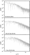 |
Fig. 10 Power spectrum of the observed TESS variations of three selected stars (gray lines). Dashed black lines denote a fit using a broken power law. |
6 Summary
We studied the photometric signatures resulting from the line-driven wind instability by applying either sinusoidal or stochastic boundary perturbations. We determined the photometric variability from mass-flux variations, assuming that the wind consists of a large number of independent conical sectors.
The calculations show that the instability already develops around the sonic point of the wind, provided that the base perturbations are comparable to (but smaller than) the thermal speed. Because the light variability originates in the subsonic part of the wind, this means that the observed light variability of O stars can be caused by wind variations if the base perturbations are sufficiently large.
We find two signatures of the line-driven wind instability in our simulated photometric data: a knee in the power spectrum of magnitude fluctuations and a negative skewness of the distribution of magnitude fluctuations. The knee can be explained by the engulfment of small-scale perturbations by large overdensities, while the negative skewness is the result of spatial dominance of rarefied regions, which leads to lower flux and higher magnitude difference. Both the knee and the negative skewness endure when combining the light curves from independent wind sectors, even for a relatively large number of sectors.
The simulated light curves are compared with TESS light curves of OB stars that show stochastic variability. The observed variations bear signatures of the line-driven wind instability. The distribution function of magnitude differences of observational light curves shows negative skewness implying more frequent periods of lower flux. Moreover, the power spectrum of a significant fraction of light curves show a knee. These observational features could be direct evidence for a ensemble of discrete overdensities embedded in large rarefied regions created by line-driven wind instability.
Although wind blanketing due to the line-driven wind instability provides a reasonable explanation of stochastic light variability of hot stars, there may be other competing processes leading to light variability, such as subsurface convection. However, additional observational tests of the mechanism ought to be undertaken. Most of the light absorbed by the wind comes from the extreme ultraviolet region (which is hardly accessible for observation). This means that far-ultraviolet photometry should mostly vary in phase with visual observations. Ultraviolet and visible variations in phase are not expected due to hot convective plumes, which are expected to be manifested mostly as temperature variations. Moreover, there are regions in the far ultraviolet domain where the flux varies in antiphase with visual variability (e.g. around 1300 Å, Krtička 2016). This provides an additional observational test of wind blanketing variability.
Acknowledgements
The authors thank Prof. Zdeněk Mikulášek for the discussion of TESS photometric light curves.This article is based upon work from the “ChETEC” COST Action (CA16117), supported by COST (European Cooperation in Science and Technology). J.K. acknowledges support by grant GA ČR 18-05665S.
References
- Abbott, D. C., & Hummer, D. G. 1985, ApJ, 294, 286 [Google Scholar]
- Aerts, C., & Rogers, T. M. 2015, ApJ, 806, L33 [Google Scholar]
- Aerts, C., Puls, J., Godart, M., & Dupret, M. A. 2009, A&A, 508, 409 [NASA ADS] [CrossRef] [EDP Sciences] [Google Scholar]
- Aerts, C., Símon-Díaz, S., Bloemen, S., et al. 2017, A&A, 602, A32 [NASA ADS] [CrossRef] [EDP Sciences] [Google Scholar]
- Benaglia, P., Vink, J. S., Martí, J., et al. 2007, A&A, 467, 1265 [NASA ADS] [CrossRef] [EDP Sciences] [Google Scholar]
- Blomme, R., Mahy, L., Catala, C., et al. 2011, A&A, 533, A4 [NASA ADS] [CrossRef] [EDP Sciences] [Google Scholar]
- Bohannan, B., Abbott, D. C., Voels, S. A., & Hummer, D. G. 1986, ApJ, 308, 728 [Google Scholar]
- Bowman, D. M., Burssens, S., Simón-Díaz, S. et al. 2020, A&A, 640, A36 [CrossRef] [EDP Sciences] [Google Scholar]
- Burssens, S., Simón-Díaz, S., Bowman, D. M., et al. 2020, A&A, 639, A81 [CrossRef] [EDP Sciences] [Google Scholar]
- Cantiello, M., Langer, N., Brott, I., et al. 2009, A&A, 499, 279 [NASA ADS] [CrossRef] [EDP Sciences] [Google Scholar]
- Carlberg, R. G. 1980, ApJ, 241, 1131 [Google Scholar]
- Castor, J. I., Abbott, D. C., & Klein, R. I. 1975, ApJ, 195, 157 [NASA ADS] [CrossRef] [Google Scholar]
- Crowther, P. A., Hillier, D. J., Evans, C. J., et al. 2002, ApJ, 579, 774 [Google Scholar]
- Crowther, P. A., Lennon, D. J., & Walborn, N. R. 2006, A&A, 446, 279 [NASA ADS] [CrossRef] [EDP Sciences] [Google Scholar]
- David-Uraz, A., Owocki, S. P., Wade, G. A., Sundqvist, J. O., & Kee, N. D. 2017, MNRAS, 470, 3672 [Google Scholar]
- Davies, B., Vink, J. S., & Oudmaijer, R. D. 2007, A&A, 469, 1045 [NASA ADS] [CrossRef] [EDP Sciences] [Google Scholar]
- Dessart, L., & Owocki, S. P. 2002, A&A, 383, 1113 [NASA ADS] [CrossRef] [EDP Sciences] [Google Scholar]
- Dufton, P. L., Ryans, R. S. I., Simón-Díaz, S., Trundle, C., & Lennon, D. J. 2006, A&A, 451, 603 [NASA ADS] [CrossRef] [EDP Sciences] [Google Scholar]
- Feldmeier, A. 1993, PhD thesis, Ludwig-Maximilians-Universität, München, Germany [Google Scholar]
- Feldmeier, A. 1995, A&A, 299, 523 [NASA ADS] [Google Scholar]
- Feldmeier, A., & Thomas, T. 2017, MNRAS, 469, 3102 [Google Scholar]
- Feldmeier, A., Puls, J., & Pauldrach, A. W. A. 1997, A&A, 322, 878 [NASA ADS] [Google Scholar]
- Feldmeier, A., Oskinova, L., & Hamann, W.-R. 2003, A&A, 403, 217 [NASA ADS] [CrossRef] [EDP Sciences] [Google Scholar]
- Haucke, M., Cidale, L. S., Venero, R. O. J., et al. 2018, A&A, 614, A91 [NASA ADS] [CrossRef] [EDP Sciences] [Google Scholar]
- Jiang, Y.-F., Cantiello, M., Bildsten, L., Quataert, E., & Blaes, O. 2015, ApJ, 813, 74 [Google Scholar]
- Kholtygin, A. F., Sudnik, N. P., Burlakova, T. E., & Valyavin, G. G. 2011, Astron. Rep., 55, 1105 [Google Scholar]
- Kourniotis, M., Bonanos, A. Z., Soszyński, I., et al. 2014, A&A, 562, A125 [NASA ADS] [CrossRef] [EDP Sciences] [Google Scholar]
- Krtička, J. 2016, A&A, 594, A75 [NASA ADS] [CrossRef] [EDP Sciences] [Google Scholar]
- Krtička, J., & Feldmeier, A. 2018, A&A, 617, A121 [NASA ADS] [CrossRef] [EDP Sciences] [Google Scholar]
- Krtička, J., & Kubát, J. 2017, A&A, 606, A31 [NASA ADS] [CrossRef] [EDP Sciences] [Google Scholar]
- Lecoanet, D., Cantiello, M., Quataert, E., et al. 2019, ApJ, 886, L15 [Google Scholar]
- Lefever, K., Puls, J., & Aerts, C. 2007, A&A, 463, 1093 [NASA ADS] [CrossRef] [EDP Sciences] [Google Scholar]
- Lucy, L. B. 1984, ApJ, 284, 351 [Google Scholar]
- Lucy, L. B., & Solomon, P. M. 1970, ApJ, 159, 879 [NASA ADS] [CrossRef] [Google Scholar]
- MacGregor, K. B., Hartmann, L., & Raymond, J. C. 1979, ApJ, 231, 514 [Google Scholar]
- Maíz Apellániz, J., Sota, A., Morrell, N. I., et al. 2013, in Massive Stars: From alpha to Omega (USA: NASA), 198 [Google Scholar]
- Markova, N., & Puls, J. 2008, A&A, 478, 823 [NASA ADS] [CrossRef] [EDP Sciences] [Google Scholar]
- Martins, F., Marcolino, W., Hillier, D. J., Donati, J. F., & Bouret, J. C. 2015, A&A, 574, A142 [NASA ADS] [CrossRef] [EDP Sciences] [Google Scholar]
- Martins, F., Schaerer, D., & Hillier, D. J. 2005, A&A, 436, 1049 [NASA ADS] [CrossRef] [EDP Sciences] [Google Scholar]
- Nazé, Y., Oskinova, L. M., & Gosset, E. 2013, ApJ, 763, 143 [Google Scholar]
- Norman, M. L., Wilson, J. R., & Barton, R. T. 1980, ApJ, 239, 968 [Google Scholar]
- Oskinova, L. M., Hamann, W.-R., & Feldmeier, A. 2007, A&A, 476, 1331 [NASA ADS] [CrossRef] [EDP Sciences] [Google Scholar]
- Owocki, S. P. 1991, in Wolf-Rayet Stars and Interrelations with Other Massive Stars in Galaxies, eds. K. A. van der Hucht, & B. Hidayat (Berlin: Springer), 143, 155 [Google Scholar]
- Owocki, S. P., & Puls, J. 1996, ApJ, 462, 894 [Google Scholar]
- Owocki, S. P., & Puls, J. 1999, ApJ, 510, 355 [NASA ADS] [CrossRef] [Google Scholar]
- Owocki, S. P., & Rybicki, G. B. 1984, ApJ, 284, 337 [Google Scholar]
- Owocki, S. P., Castor, J. I., & Rybicki, G. B. 1988, ApJ, 335, 914 [Google Scholar]
- Pedersen, M. G., Chowdhury, S., Johnston, C., et al. 2019, ApJ, 872, L9 [Google Scholar]
- Poe, C. H., Owocki, S. P., & Castor, J. I. 1990, ApJ, 358, 199 [Google Scholar]
- Ramiaramanantsoa, T., Moffat, A. F. J., Harmon, R., et al. 2018, MNRAS, 473, 5532 [Google Scholar]
- Reeve, D. C., & Howarth, I. D. 2016, MNRAS, 456, 1294 [NASA ADS] [CrossRef] [Google Scholar]
- Ricker, G. R., Winn, J. N., Vanderspek, R., et al. 2015, J. Astron. Teles. Instrum. Syst., 1, 014003 [Google Scholar]
- Simón-Díaz, S., Aerts, C., Urbaneja, M. A., et al. 2018, A&A, 612, A40 [NASA ADS] [CrossRef] [EDP Sciences] [Google Scholar]
- Stone, J. M., & Norman, M. L. 1992, ApJS, 80, 753 [Google Scholar]
- Sundqvist, J. O., & Owocki, S. P. 2015, MNRAS, 453, 3428 [Google Scholar]
- Sundqvist, J. O., Owocki, S. P., & Puls, J. 2018, A&A, 611, A17 [NASA ADS] [CrossRef] [EDP Sciences] [Google Scholar]
- Šurlan, B., Hamann, W.-R., Aret, A., et al. 2013, A&A, 559, A130 [NASA ADS] [CrossRef] [EDP Sciences] [Google Scholar]
- ud-Doula, A., & Owocki, S. P. 2002, ApJ, 576, 413 [Google Scholar]
- van Leer, B. 1977, J. Comput. Phys., 23, 276 [Google Scholar]
Mikulski Archive for Space Telescopes, https://archive.stsci.edu
All Figures
 |
Fig. 1 Snapshot of height variations of the wind velocity (black lines) and density (gray lines) compared with the stationary CAK solution (dashed lines), plotted for sinusoidal base perturbation (upper panel) and for the Langevin base perturbation (lower panel). Calculations are performed in non-dimensional units with velocity expressed in units of the thermal speed. |
| In the text | |
 |
Fig. 2 Variability of the mass flux at u = 1∕3, u = 1, and u = 5 (increasing amplitude) for sinusoidal (upper panel) and Langevin base perturbations (lower panel). Calculations are performed in nondimensional units with stationary mass flux ρu = 1. |
| In the text | |
 |
Fig. 3 Light variability for sound wave (upper panel) and Langevin boundary perturbations (bottom panel). Individual curves are calculated from the mass flux variations for velocities u = 1∕3, u = 1, and u = 5. The graph shows the difference between actual magnitude and magnitude predicted for the mean flux. |
| In the text | |
 |
Fig. 4 Histograms of the distribution of magnitude differences for sound wave perturbations (upper panel) and Langevin perturbations (bottom panel), for u = 1∕3, 1, and 5. The ordinate gives the relative frequency divided by the box width, i.e, the distribution function. It is normalised in such a way that its integral over all magnitude differences is unity. |
| In the text | |
 |
Fig. 5 Power spectrum of light variability for Langevin base perturbations, for velocities u = 1∕3 and u = 5. Determined as a magnitude of the coefficients of the Fourier transform of the light curves. |
| In the text | |
 |
Fig. 6 Light variability for sound wave perturbations (upper panel) and Langevin perturbations (bottom panel) summed over N = 103 independent cones, calculated from mass flux variations for u = 1∕3, 1, and 5. The graph shows the difference between actual magnitude and mean. |
| In the text | |
 |
Fig. 7 Histogram of the distribution of magnitude differences for sound wave perturbations (upper panel) and Langevin perturbations (bottom panel) summed over N = 103 independent cones, calculated from mass flux variations at u = 1∕3, 1, and 5. |
| In the text | |
 |
Fig. 8 Power spectrum derived from the light curve summed over N = 300 and N =103 independent cones (given in Fig. 6) for the case of Langevin base perturbation at velocity u = 5. |
| In the text | |
 |
Fig. 9 Distribution of flux variations of TESS observations |
| In the text | |
 |
Fig. 10 Power spectrum of the observed TESS variations of three selected stars (gray lines). Dashed black lines denote a fit using a broken power law. |
| In the text | |
Current usage metrics show cumulative count of Article Views (full-text article views including HTML views, PDF and ePub downloads, according to the available data) and Abstracts Views on Vision4Press platform.
Data correspond to usage on the plateform after 2015. The current usage metrics is available 48-96 hours after online publication and is updated daily on week days.
Initial download of the metrics may take a while.


