| Issue |
A&A
Volume 648, April 2021
|
|
|---|---|---|
| Article Number | A68 | |
| Number of page(s) | 9 | |
| Section | Atomic, molecular, and nuclear data | |
| DOI | https://doi.org/10.1051/0004-6361/202038941 | |
| Published online | 12 April 2021 | |
Empirical determination of atomic line parameters of the 1.5 μm spectral region
1
Instituto de Astrofísica de Canarias (IAC),
Vía Láctea s/n,
38205
San Cristóbal de La Laguna,
Tenerife,
Spain
e-mail: This email address is being protected from spambots. You need JavaScript enabled to view it.
; This email address is being protected from spambots. You need JavaScript enabled to view it.
; This email address is being protected from spambots. You need JavaScript enabled to view it.
2
Departmento Astrofísica, Universidad de La Laguna,
38205
San Cristóbal de La Laguna,
Tenerife,
Spain
Received:
15
July
2020
Accepted:
25
February
2021
Abstract
Context. Both the quality and amount of astrophysical data are steadily increasing over time owing to the improvement of telescopes and their instruments. This requires corresponding evolution of the techniques used for obtaining and analyzing the resulting data. The infrared spectral range at 1.56 μm usually observed by the GRegor Infrared Spectrograph (GRIS) at the GREGOR solar telescope has a width of around 30 Å and includes at least 15 spectral lines. Normally, only a handful of spectral lines (five at most) are used in studies using GRIS because of the lack of atomic parameters for the others. Including more spectral lines may alleviate some of the known ambiguities between solar atmospheric parameters.
Aims. We used high-precision spectropolarimetric data for the quiet Sun at 1.56 μm observed with GRIS on the GREGOR along with the SIR inversion code in order to obtain accurate atomic parameters for 15 spectral lines in this spectral range.
Methods. We used inversion techniques to infer both solar atmospheric models and the atomic parameters of spectral lines which, under the local thermodynamic equilibrium approximation, reproduce spectropolarimetric observations.
Results. We present accurate atomic parameters for 15 spectral lines within the spectral range from 15 644 to 15 674 Å. This spectral range is commonly used in solar studies because it enables the study of the low photosphere. Moreover, the infrared spectral lines are better tracers of the magnetic fields than the optical ones.
Key words: atomic data / methods: observational / line: profiles / techniques: polarimetric / Sun: photosphere
© ESO 2021
1 Introduction
Light is the most powerful tool for getting information from astronomical bodies. Physical conditions of the emitting object are encoded in the light emitted. Using spectroscopy, for example, it is possible to identify the elements present in stellar atmospheres simply by looking for their signatures in the spectra. These signatures are the spectral lines formed by transitions between the energy states of an atom.
Many efforts have been made to characterize spectral lines. In the gathering of information about spectral lines, it is inescapable to cite the work of Moore et al. (1966) and subsequent databases such as NIST (Kramida et al. 2019), VALD (Piskunov et al. 1995), and CHIANTI (Dere et al. 1997). One of the key points in these studies is the oscillator strength of the spectral line f, which can be defined as the ratio between the probability of absorption or emission of electromagnetic radiation in a transition between energy levels of an atom or molecule and the probability of this transition in a classical oscillator (Mihalas 1978). Two important international collaborations have been created in order to calculate and collect oscillator strengths of astrophysical interest: the Opacity Project (Seaton et al. 1994) and the FERRUM project (Johansson 2002), specializing in iron.
In general, there are three ways of calculating oscillator strengths: theoretical, semi-empirical, and observational. A good description of the theoretical and semi-empirical methods can be found in Borrero et al. (2003) and references therein.
Observationally, it is possible to determine the oscillator strengths using solar spectra. The basic idea is to use a model atmosphere and solve the radiative transfer equation (RTE), allowing the oscillator strength value to be a free parameter in order to make the synthetic spectra agree with solar spectrum. It is important to stress that the results achieved using these studies rely on having suitable atmospheric models, line damping parameters, solar abundance elements, and so on.
The first successful attempt at determining oscillator strengths from solar spectra was by Gurtovenko & Kostic (1981, 1982), who used the model atmosphere of Holweger & Müller (1974) to fit the central intensity of 865 Fe I spectral lines (between 4000 and 8000 Å) to the solar atlas (Delbouille et al. 1973). The same atlas was used by Thévenin (1989, 1990) to determine the oscillator strength of thousands of spectral lines from 4006 to 7950 Å. These latter authors used the model atmosphere of Gustafsson et al. (1975) in order to fit either the central core and the beginning of the wings or the central depth of the line. Those works compared some of their results with theoretical calculations (Blackwell et al. 1976, 1979) and revealed a high degree of agreement.
One step further was taken by Borrero et al. (2003), who introduced such improvements as fitting the whole spectral line, as opposed to fitting some points of the line; using broadening collisional parameters (Anstee & O’Mara 1995; Barklem & O’Mara 1997; Barklem et al. 1998) where previous works had used the Unsöld formula with correction factors; and using a two-component model atmosphere to simulate granular and intergranular behavior (Borrero & Bellot Rubio 2002). Socas Navarro (2011) used the same procedure but with a model atmosphere of a single component to calculate the oscillator strength of the Fe I 6302.5 Å spectral line used by the solar optical telescope on the Hinode satellite (Kosugi et al. 2007; Ichimoto et al. 2008; Shimizu et al. 2008; Suematsu et al. 2008; Tsuneta et al. 2008). This oscillator strength value was used by Socas Navarro (2015) to determine the oxygen abundance in the solar photosphere.
In this paper, we wish to make our contribution to this effort by observationally determining accurate parameters for 15 spectral lines of the 1.56 μm spectral region (Fig. 1). In this spectral region, the main contributor to the solar continuum opacity, the H- ion, reaches the minimum of opacity. It therefore allows us to probe the deepest layers of the solar photosphere (Gray 2008). Furthermore, infrared spectral lines are better tracers of magnetic fields than optical ones because the ratio between theZeeman splitting and the width of the line is proportional to the wavelength (Bellot Rubio & Orozco Suárez 2019).
Because of the high inhomogeneity of the solar photosphere and the nonlinearity of the RTE, there is no single model atmosphere capable of explaining an averaged spectrum over a large area of the solar disk. This may lead to inaccuracies when calculating oscillator strengths. Therefore, our approach to solve the problem is based on using not only a single solar spectrum but also spatially resolved pixel-by-pixel observations (0.135′′ × 0.135′′). Thus, we have a large number of values for the oscillator strength from which we can calculate the mean and standard deviation for each spectral line.
We use spectropolarimetric inversions for this work. In solar physics, many computer codes have been developed for spectropolarimetric inversions (e.g., HAZEL: Asensio Ramos et al. 2008, SPINOR: Frutiger & Solanki 1998, SIR: Ruiz Cobo & del Toro Iniesta 1992, and NICOLE: Socas Navarro et al. 2000). These codes try to find reliable physical quantities for the solar atmosphere from a set of observed Stokes parameters. To this end, the difference between observed and synthetic spectra is minimized. The synthetic spectrum is numerically calculated from a simplified model atmosphere by solving the RTE.
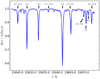 |
Fig. 1 Region of the FTS atlas of Wallace et al. (2011). The spectral lines marked with arrows have been included in this study. |
2 Observations and data reduction
On 2018 August 29, December 14, and December 17, the four Stokes parameters of the spectral lines at 1.56 μm (from 15 644 to 15 674 Å) were recorded using the Tenerife Infrared Polarimeter working with GRIS (Collados et al. 2007, 2012) attached to the German GREGOR telescope (Schmidt et al. 2012). The data sets were obtained in a quiet Sun region located at disk center. The spectral sampling was 40.00 mÅ. A spatial resolution of 0.5′′ was reached through the adaptive optics system (Berkefeld et al. 2016) locked on granulation. Figure 2 shows the high quality of the data.
The maps we present here (three, one per day mentioned above) cover a scanned area of about 62.0′′ × 54.0′′ with an integration time of 2 s per slit position (the total cadence was ~3.6 s per slit position due to overheads). The slit position was aligned with the solar north–south direction and the Sun was scanned in a perpendicular direction to the slit with a step size of 0.135′′. The contrast of the continuum image – defined as the standard deviation of the full map divided by its average value – is 2.7 per cent.
The data were demodulated with dedicated software (Schlichenmaier & Collados 2002). This software also corrects for bias, flatfield, and bad pixels and removes the instrumental cross-talk. Additional corrections were applied to the data:
-
We corrected for wavelength-independent stray light by subtracting a veil quantity (Iv) from our intensity spectrum:
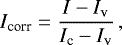 (1)
(1)where Ic stands for the continuum intensity and Icorr for the veil-corrected spectrum. In order to infer the veil, we fit the average intensity spectrum to that of the Fourier Transform Spectrometer (FTS) of Wallace et al. (2011). As the FTS spectrum has higher spectral resolution, we convolved it with a Gaussian function with a standard deviation σ that will be representative of our spectral resolution. We then inferred the value of both σ and the veil by minimizing the quadratic difference between our average Stokes I and the convolved atlas. The σ was 81.26 mÅ and the veil was 2.5%. We used these numbers to correct each Stokes I profile.
After the standard reduction, the continuum is not flat but has some undulations. We fit a high-order polynomial to the continuum wavelengths and divide by it. All Stokes profiles were normalized accordingly.
-
We removed the residual cross-talk from Stokes I from Stokes Q, U, and V. We calculated the mean value in the continuum spectral region for each pixel and the polarization profiles. In the Zeeman effect, there is no continuum polarization, and we do not expect the continuum to be polarized by scattering at such a long wavelength. Assuming that the polarized continuum should be zero, we then calculated the correction factor δ for the cross-talk from intensity as follows:
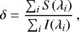 (2)
(2)where S runs the Q, U, and V polarization profiles, and the sub-index i contains the selected continuum wavelengths. S(λc) and I(λc) represent mean values in the continuum region. Finally, the cross-talk correction is:
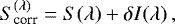 (3)
(3) We denoised the data using a principal component analysis (PCA; Loève 1975; Rees & Guo 2003). This technique is used to reduce the uncorrelated noise but not the systematic errors. It works by decomposing the data set into its principal components or eigenvectors and sorting them by their eigenvalues. The data can then be rebuilt using just the eigenvectors with highest eigenvalues (see Martínez González et al. 2008a,b for more details).
We corrected for polarized interference fringes. The fringing of charge coupled device (CCD) detectors occurs because of interference between the incident light and the light internally reflected at the interfaces between the thin layers of the CCD. Fringes can be observed easily after PCA denoising, and they change with time and slit position. We removed them by fitting, pixel by pixel, a sinusoidal function to the blue and red continuum close to each spectral line. These two sinusoidal functions usually havedifferent frequencies or amplitudes, and so we linearly interpolate from one function to the other in order to discover how fringes affect each spectral line region. In Fig. 3 we show an example of a Stokes Q map at time-step 300, before (left) and after (right) fringe removal.
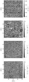 |
Fig. 2 Intensity and polarization maps of dataset 1 observed on 2018 August 29. |
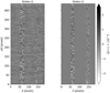 |
Fig. 3 Stokes Q map for time-step number 300 after applying PCA denoising, before (left) and after (right) fringe removal. |
3 Determination of atomic parameters
Historically, the spectral lines in the visible spectral range have been studied in depth in the laboratory, but experimental data are lacking for the infrared part of the spectrum. When there are no accurate laboratory measurements of atomic parameters for certain transitions, such as the oscillator strength, the solar spectrum can be used to infer them. Previous works fixed the model atmosphere and performed an inversion of the observed spectrum with the oscillator strength as the only free parameter (Gurtovenko & Kostic 1981, 1982; Thévenin 1989, 1990; Borrero et al. 2003). The reason for fixing the model atmosphere is that the oscillator strength and certain atmospheric parameters, mainly the temperature, are degenerate. For instance, the temperature is degenerate with the oscillator strength because it influences the strength of the spectral line; temperature determines the number density of neutral iron atoms, the number density of the atoms excited to the lower level of the transition, the gradient of the source function, and so on.
In this work, we propose an iterative method in which the model atmosphere and the oscillator strength are inferred simultaneously. In one iteration we fix the model atmosphere, in the next we fix the oscillator strength, and so on. Thus, we search for the best possible match between the synthesis and the observation. Furthermore, we apply this to a large number of spectra emerging from 1D atmospheres corresponding to the individual pixels. Hence, statistically this method should be more robust than in previous works.
The SIR (Stokes Inversion based on Response Functions) code (Ruiz Cobo & del Toro Iniesta 1992) was used to invert our spectropolarimetric data. This code allows us to synthesize and invert spectral lines under the assumption of local thermodynamic equilibrium (LTE; when collisional transitions dominate over radiative ones, e.g., in solar photospheric layers) by solving the RTE for polarized light:
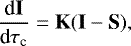 (4)
(4)
where τc is the optical depth at the continuum wavelength, I and S are the pseudo-vectors of the Stokes parameters and the source function, respectively, and K stands for the propagation matrix defined as
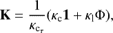 (5)
(5)
where 1 and Φ are the identity and line absorption matrixes, κc and  stand for the continuum opacity and the continuum opacity evaluated at the reference wavelength, and κl is the line opacity given by
 (6)
(6)
where  is the line absorption coefficient and
  stands for the stimulated emission coefficient. Through the comparison of the RTE derived from quantum mechanics and derived from the classical physics (more details in Landi Degl’Innocenti & Landolfi 2004), the line absorption coefficient can be written in the form
 (7)
(7)
where e0 is the absolute value of the electron charge, Nl is the number of atoms per unit volume in the lower level of the transition, m and c are the electron mass and the speed of light, and f(αlJl → αuJu) is the oscillator strength of the transition.
The strength of a spectral line, defined as the area under or above (i.e., emission or absorption) the curve described for the spectral line in a wavelength versus intensity plot, depends on the product Agf, where A is the abundance (related to Nl in Eq. (7)). The oscillator strength f is the correction factor when we express the probability of absorption of electromagnetic radiation in terms of the degeneracy of the lower level g and the transition probability of a harmonic oscillator (Mihalas 1978). As can be seen in Eqs. (4)–(7), both the abundance and oscillator strength affect the RTE. Consequently, accuracy in the determination of these quantities is key to getting accurate results in the inversions.
The parameter commonly used for the synthesis of spectral lines is the logarithm of the product of the lower level degeneracy multiplied by the oscillator strength log (gf). The abundance has to be fixed in order to calculate the oscillator strength. We therefore take the abundances from Asplund et al. (2009).
We use the coefficients for collisional broadening from the ABO theory (Anstee & O’Mara 1991, 1995; Barklem & O’Mara 1997; Barklem et al. 1998), where σ and α stand for the line broadening cross section and velocity parameter, respectively. The coefficients presented in Table 1 were calculated by Barklem (priv. comm.).
3.1 Models
SIR uses an hermitian method to integrate the RTE for polarized light (Bellot Rubio et al. 1998). The great accuracy and speed reached by an hermitian method is shown in de la Cruz Rodríguez & Piskunov (2013), although, following their calculations, a method based on Diagonal Element Lambda Operator (DELO) with cubic Bezier interpolation of the source function can in some cases reach a better accuracy, mainly in chromospheric layers. Nevertheless, the accuracy gain depends on the smoothness of the different physical quantities with depth, and for photospheric lines an hermitian method behaves even better than a cubic Bezier method. For an in-depth analysis of the performance of different integration schemes see Janett et al. (2017) and Janett & Paganini (2018). Bellot Rubio et al. (1998) calculate an accuracy better than 10−5 for integration of Stokes I and 10−6 the other Stokes profiles when a step size of 0.1 in the logarithm of continuum optical depth is chosen. Consequently, in this paper we have used models with 55 points in depth, from 1.4 to −4.0 in log (τ) with a step size of 0.1. As a boundary condition for the integration of the RTE, SIR uses a diffusion approximation; that is, at the bottom of the atmosphere, the first point in the grid model, the Stokes vector is approximated by:
 (8)
(8)
where Sν = (Bν, 0, 0, 0).
The models have three quantities that are independent of depth, namely macroturbulence velocity, filling factor, and stray light contamination (not used in this work), and also 11 depth-dependent quantities, namely the logarithm of line-of-sight continuum optical depth at 5000 Å, temperature (T), electron pressure (Pe), microturbulence velocity, magnetic field (strength, inclination, and azimuth), line-of-sight velocity, geometrical height (z), gas density (ρ), and gas pressure (Pg). Not all these quantities are completely independent: z, ρ, and Pg are evaluated from T and Pe. Additionally, although SIR can allow the determination of Pe as a free parameter, we have chosen the hydrostatic equilibrium option: Pe is calculated from T and abundances assuming hydrostatic equilibrium through the ideal gas law assuming a Pg value at the upper boundary of the atmosphere. In order to evaluate the electron number density, SIR uses Saha’s equation for 28 elements, H−, and H and He molecules. As in this equation the ion populations depend on electron density, SIR uses an iterative procedure based on Mihalas (1967). A detailed description of the state equation and the algorithm used to determine partial pressures, damping parameters, and continuum absorption coefficient can be found in Wittmann (1974).
3.2 Estimation of log(gf) values
As the initial step, for each dataset we inferred log (gf) of the 15 662.017 Å line from its intensity profile averaged over the field of view. This line was selected as it is the strongest. The model atmosphere was fixed to model C of Fontenla et al. (1993) (FALC), which is a semi-empirical stratified model tuned to reproduce the solar quiet spectrum. After several inversion runs looking for the most suitable macroturbulence velocity, a fixed value of 0.92 km s−1 was found to be optimum. From these three inversions, an average value of log (gf) = 0.140 ± 0.018 was obtained.
Subsequently, we performed inversions of these intensity-averaged profiles (three, one per data set) using the FALC model as an initial atmospheric model but fixing log (gf) to the previously obtained value. The stratifications of the temperature and line-of-sight velocity of the model were modified during the inversion. Through the inversion, a more suitable model is obtained which is used to recalculate the log (gf) value for this spectral line.
This whole process was repeated iteratively to find the value of log (gf) and the atmospheric model that minimize the difference between the observed and synthetic spectrum.
Figure 4 shows the temperature and line-of-sight velocity of FALC and the new model for comparison. The temperatureof both models is very similar. However, a linear gradient along the optical depth of the line-of-sight velocity is needed to fit the observations. This gradient is the result of the known asymmetry produced in the presence of granules and intergranules in the averaged spectra.
Using this new model, the oscillator strength of two more spectral lines (at 15 648.514 and 15 652.873 Å) could be calculated using log (gf) as a free parameter in the synthesis. Figure 5 shows the fits between the observation and the synthesis for the three spectral lines. The mean and the standard deviation of the log (gf) values for the three measurements and for each line are: − 0.596 ± 0.007 for the line at 15 648.514 Å, − 0.025 ± 0.003 for the line at 15 652.873 Å, and 0.187 ± 0.012 for the line at 15 662.017 Å. Inversion uncertainties in the determination of log (gf) values were calculated for the line at 15 662.017 Å resulting in 0.010. Thus, the inversion uncertainties (i.e., the sensitivity of the spectral line to changes in the log (gf) values) are contained in the errorsof the log (gf) calculation we present here. As can be seen in Fig. 5, the observed profiles are well reproduced for the synthesis.
At this point we faced the problem of the degeneracy between temperature and log (gf) values. As explained above, the high inhomogeneity of the solar photosphere and the nonlinearity of the RTE may lead to inaccuracies in model atmosphere determination. Changes in temperature affect the number of absorbents that produce the spectral lines (Nl in Eq. (7)). Furthermore, the source function (S in Eq. (4)) in LTE conditions is the Planck function, which is related to the temperature. The effects produced by temperature may be compensated for by changing the log (gf) values in order to fit the observation (e.g. as seen in Eq. (7)). The difference in temperature at the solar photosphere between granules and intergranular lanes could reach around 1000 K (Ruiz Cobo et al. 1996), but fluctuations in temperature will be smaller inside each pixel on the plane of the sky. We therefore used the highest-quality data set (the one recorded on 2018 August 29) for doing inversions pixel by pixel to overcome this problem. Thus, we obtained log (gf) values with different temperatures and we were able to calculate the mean value and standard deviation.
To this end, a new inversion was done using the three spectral lines with their now known log (gf) values (hereinafter, main spectral lines). The strategy followed to do the inversions was the same as before (explained in Appendix B). Hereafter, the model used to perform the fit consists of two 1D atmospheres (magnetized and nonmagnetized). It is necessary to include the magnetized atmosphere because the magnetic field affects abundances determination (Borrero 2008). Moreover, we included the Stokes Q, U, and V parameters for the 15 648.514 Å spectral line (i.e., the spectral line with highest magnetic sensitivity) in the inversions to provide more information. Thus, log (gf) values are more constrained. The 400 pixels with the best χ2 between the observation and the synthesis were chosen from the inversion. Two atmosphericmodels were obtained for each pixel. These models were used to calculate log (gf) for each line within the GRIS spectra around 1.56 μm pixel by pixel. Thus, it was possible to redetermine the log (gf) values of the main spectral lines and get a first approximation for the log (gf) values for the remaining spectral lines.
Finally, the log (gf) values of the 15 spectral lines obtained in the previous step were used to perform a new inversion. The models retrieved in this inversion were used to redetermine the log (gf) values of all the spectral lines.
Figure 6 shows the histograms of the log (gf) values for three spectral lines. The plots were made using the 400 best pixels with the best χ2 between the synthesis and the observation, as noted before. In order to show the adequacy of the method, a Gaussian function is plotted over the histogram with the mean and standard deviation values calculated for the log (gf) value for each spectral line.
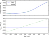 |
Fig. 4 Comparison between FALC and the new model in temperature (top) and line-of-sight velocity (bottom). The solid blue line represents the FALC model. The dashed green line represents the new model. |
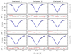 |
Fig. 5 Fits between the observation (black points) and the synthesis (blue solid lines) of each data set and each spectral line. The residuals are shown as a solid red line. |
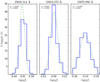 |
Fig. 6 log (gf) histograms (blue solid line) for three spectral lines (from left to right: 15 648.514, 15 652.873, and 15 670.998 Å). The dashed green line is a Gaussian function with the mean value and standard deviation of log (gf). |
Atomic line parameters of the 1.5 μm spectral region.
3.3 Dealing with blends
Blends occur when two or more spectral lines are so close together that they are impossible to study separately. In this work we faced two types of blends:
Secondary line over the wing of a principal line: The log (gf) of the principal spectral line was calculated with the method explained above but excluding the wing contaminated by the blend. The log (gf) value of the principal spectral line was fixed in order to get the log (gf) value of the secondary line.
Secondary and principal line almost sharing the central wavelength: Firstly, the range of log (gf) of the principal and secondary lines were calculated separately. This range is delimited by two values. The upper bound of the log (gf) of the principal line is given by the difference in depth between the synthesized and the observed line. The lower bound occurs when the synthetic line by itself is below the noise level. Secondly, log (gf) values of the principal line were fixed and the log (gf) values of the secondary line were found using the difference between the synthesis and the observations (χ2) for a large number of pixels. Finally, the two values that minimized the χ2 were selected.
3.4 Discussion of results
The log (gf) values calculated in this work are listed in Table 1 and the whole iterative process is depicted in Fig. 7.
The results obtained for the log (gf) values are in accordance with those previously calculated in the literature. For example, the log (gf) values for the spectral lines at 15 648.514 and 15 652.873 Å calculated by Borrero et al. (2003) are −0.675 and −0.043 respectively.In their work, those authors used an Fe abundance of 7.43 dex (Bellot Rubio & Borrero 2002). However, we used an Fe abundance of 7.50 dex (Asplund et al. 2009), which gives log (gf) values of −0.745 and −0.113, very close to the values of this work.
It is important to stress that the values for the oscillator strengths presented in this work were calculated with the abundances from Asplund et al. (2009): 7.50, 8.69, and 4.95 dex for iron (Fe), oxygen (O), and titanium (Ti), respectively. Oscillator strength values are useless in observational studies without their corresponding abundances. If the abundances are changed, the values of the oscillator strengths must be changed proportionately.
The excellent agreement with previous works and the low values of the uncertainties found here are good indicators of the quality of the method. Moreover, the residuals –defined as the difference between observed and synthetic spectra– resulting in the last inversion given in Fig. 8 prove the adequacy of the models inferred.
The uncertainties are higher for the secondary spectral lines in blends (see Table 1). This was expected because they have a small influence on the inverted model atmosphere owing to their low significance in the conditions of temperatureand electronic density where the spectrum is formed in the solar atmosphere.
As mentioned above, the coefficients for collisional broadening come from the ABO theory (Anstee & O’Mara 1991, 1995; Barklem & O’Mara 1997; Barklem et al. 1998), but it was not possible to calculate coefficients with asterisks in Table 1. In these cases, values of the order of known values were taken. Therefore, more accurate log (gf) values for the secondary spectral lines in blends could be reached with the real values of the σ and α coefficients.
Figure 9 shows an example of the fits acquired through the last inversion. The high quality of the fits between the observation and the synthesis can be observed.
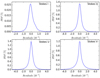 |
Fig. 7 Scheme of the process. In step 1, three averaged profiles coming from three different data sets, together with the FalC model,are used to calculate the oscillator strengths of three spectral lines. In step 2, pixel-by-pixel inversions are done using the oscillator strengths of the three spectral lines calculated previously and the data set with the highest quality to determine the oscillator strengths of 15 spectral lines. In step 3, step 2 is repeated but taking into account 15 spectral lines in the inversions to redetermine the oscillator strengths of all the spectral lines. |
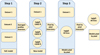 |
Fig. 8 Residuals of the whole map resulting from the last inversion. Upper panels: residuals for Stokes I (left) and Stokes Q (right). Lower panels: residuals for Stokes U (left) and Stokes V (right). |
4 Conclusions
We have developed a method for determining accurate log (gf) values for 15spectral lines in the 1.56 μm spectral region from observed solar spectroscopic data. This spectral range is usually observed with GRIS at the GREGOR telescope. We used very high-quality spectropolarimetric data, the SIR inversion code, and the coefficients for collisional broadening. The method is an iterative process. It starts from the FALC model and the averaged intensity profile of observations. It finds both model atmospheres and log (gf) values which minimize the difference between the synthesis and the observation.
We hope this study will be very useful for the community, not only for the parameters but for the method itself, because it can be easily used for other spectral lines.
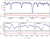 |
Fig. 9 Fits achieved in the last inversion step between the observation (black points) and the synthesis (blue solid lines) in a single pixel. Upper panel: intensity profiles. Lower panel: stokes Q, U, and V of the 15 648.514 Å spectral line. The residuals are shown with a red solid line. |
Acknowledgements
The authors are especially grateful to Paul Barklem, Manuel Collados Vera, Jesús Plata Suárez, Ivan Milić and Terry Mahoney for very interesting discussions and comments to improve the manuscript. We acknowledge financial support from the Spanish Ministerio de Ciencia, Innovación y Universidades through project PGC2018-102108-B-I00 and FEDER funds. J.C.T.A. acknowledges financial support by the Instituto de Astrofísica de Canarias through Astrofísicos Residentes fellowship. M.J.M.G. acknowledges financial support through the Ramón y Cajal fellowship. The observations used in this study were taken with the GREGOR telescope, located at Teide observatory (Spain). The 1.5-metre GREGOR solar telescope was built by a German consortium under the leadership of the Leibniz-Institute for Solar Physics (KIS) in Freiburg with the Leibniz Institute for Astrophysics Potsdam, the Institute for Astrophysics Göttingen, and the Max Planck Institute for Solar System Research in Göttingen as partners, and with contributions by the Instituto de Astrofísica de Canarias and the Astronomical Institute of the Academy of Sciences of the Czech Republic. This paper made use of the IAC Supercomputing facility HTCondor (http://research.cs.wisc.edu/htcondor/), partly financed by the Ministry of Economy and Competitiveness with FEDER funds, code IACA13-3E-2493.
Appendix A Effective Landé factor of the Fe I 15 652.873 Å spectral line
The pair of Fe I spectral lines at 15 648.514 and 15 652.873 Å has been used often since its interesting diagnostic capabilities were first probed (Solanki et al. 1992). The common value in the literature for the effective Landé factor of the Fe I line at 15 652.873 Å is 1.53 (Solanki et al. 1992). However, we recalculated all the atomic parameters of this line and found a slightly higher effective Landé factor of 1.67. Provided the lower energy level of the line has an L-S coupling scheme, we can use Eq. (A.1) to calculate its Landé factor:
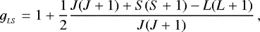 (A.1)
(A.1)
where L and S stand for the total orbital angular momentum and the total spin, respectively, and J is the total angular momentum. On the other hand, the upper energy level has a jK coupling scheme, therefore we used Eq. (A.2) (Landi Degl’Innocenti & Landolfi 2004) to calculate its Landé factor:
 (A.2)
(A.2)
where L1 and S1 are the orbital angular and spin momentum of the ‘parent’ energy level. J1 is the total angular momentum of that level which is coupled with the orbital momentum l of a further electron to give an angular momentum K. Lastly,
K is coupled with the electron spin to give the total angular momentum J (see Landi Degl’Innocenti & Landolfi (2004) for details).
In Eq. (A.2), γ is:
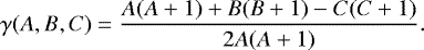 (A.3)
(A.3)
Finally, we obtained the effective Landé factor of the transition using Eq. (A.4).
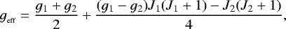 (A.4)
(A.4)
where g1 and g2 are the Landé factors of the lower and upper energy levels, respectively.
Appendix B Inversion strategy
The inversion strategy relied on a free node configuration, which means that the inversion code takes as many nodes as it needs, taking into account the data and response functions (i.e., the sensitivity of each Stokes parameter to each atmospheric quantity). SIR uses an algorithm that determines the optimum number of nodes for each quantity as a function of the number of zeros of the derivative of the chi-squared (more details in del Toro Iniesta & Ruiz Cobo 2016):
![Mathematical equation: \begin{equation*} \frac{\partial\chi^{2}}{\partial x_{m}} = \frac{2}{N_{f}}\sum_{s=0}^{3}\sum_{i=1}^{q}[I_{s}^{\textrm{obs}}(\lambda_{i})- I_{s}^{\textrm{syn}}(\lambda_{i};x)]w_{s,i}^{2}R_{m,s}(\lambda_{i}), \end{equation*}](/articles/aa/full_html/2021/04/aa38941-20/aa38941-20-eq16.png) (B.1)
(B.1)
where Nf stands for the number of degrees of freedom (i.e., the difference between the number of observables and that of the free parameters),  and
and  are the observation and the synthesis, respectively,
  are the weights (for taking into account the errors in observations, but they are normally kept at unity), and Rm,s(λi) are the response functions.
Fits achieved using the free node configuration are slightly better than limiting the number of nodes by hand. Moreover, even though we give such freedom to the code, the number of nodes selected by SIR is low (normally between 1 and 5 nodes for each quantity) and the resulting atmospheric models are smooth. The filling factor α is also inverted to evaluate the fraction of the resolution element occupied by the magnetic atmosphere.
References
- Anstee, S. D.,& O’Mara, B. J. 1991, MNRAS, 253, 549 [Google Scholar]
- Anstee, S. D.,& O’Mara, B. J. 1995, MNRAS, 276, 859 [Google Scholar]
- Asensio Ramos, A., Trujillo Bueno, J., & Landi Degl’Innocenti, E. 2008, ApJ, 683, 542 [Google Scholar]
- Asplund, M., Grevesse, N., Sauval, A. J., & Scott, P. 2009, ARA&A, 47, 481 [NASA ADS] [CrossRef] [Google Scholar]
- Barklem, P. S., & O’Mara, B. J. 1997, MNRAS, 290, 102 [Google Scholar]
- Barklem, P. S., O’Mara, B. J., & Ross, J. E. 1998, MNRAS, 296, 1057 [Google Scholar]
- Beck, C., & Choudhary, D. P. 2019, ApJ, 874, 6 [Google Scholar]
- Bellot Rubio, L. R., & Borrero, J. M. 2002, A&A, 391, 331 [NASA ADS] [CrossRef] [EDP Sciences] [Google Scholar]
- Bellot Rubio, L. R., & Orozco Suárez, D. 2019, Liv. Rev. Sol. Phys., 16, 1 [Google Scholar]
- Bellot Rubio, L. R., Ruiz Cobo, B., & Collados, M. 1998, ApJ, 506, 805 [Google Scholar]
- Berkefeld, T., Schmidt, D., Soltau, D., et al. 2016, Astron. Nachr., 333, 863 [Google Scholar]
- Blackwell, D. E., Ibbetson, P. A., Petford, A. D., & Willis, R. B. 1976, MNRAS, 117, 219 [Google Scholar]
- Blackwell, D. E., Ibbetson, P. A., Petford, A. D., & Shallis, M. J. 1979, MNRAS, 186, 633 [NASA ADS] [CrossRef] [Google Scholar]
- Borrero, J. M. 2008, ApJ, 673, 470 [Google Scholar]
- Borrero, J. M., & Bellot Rubio, L. R. 2002, A&A, 385, 1056 [NASA ADS] [CrossRef] [EDP Sciences] [Google Scholar]
- Borrero, J. M., Bellot Rubio, L. R., Barklem, P. S., & del Toro Iniesta, J. C. 2003, A&A, 404, 749 [NASA ADS] [CrossRef] [EDP Sciences] [Google Scholar]
- Collados, M., Lagg, A., Díaz García, J. J., et al. 2007, ASP Conf. Ser., 368, 611 [Google Scholar]
- Collados, M., López, R., Páez, E., et al. 2012, Astron. Nachr., 333, 872 [Google Scholar]
- de la Cruz Rodríguez, J., & Piskunov, N. 2013, ApJ, 764, 33 [NASA ADS] [CrossRef] [Google Scholar]
- Delbouille, L., Roland, G., Neven, L., & Roland, G. 1973, Atlas photometrique du spectre solaire de [lambda] 3000 a [lambda] 10000 (Belgium: Institut d’Astrophysique de l’Université de Liège) [Google Scholar]
- del Toro Iniesta, J. C., & Ruiz Cobo, B. 2016, Liv. Rev. Sol. Phys., 13, 84 [Google Scholar]
- Dere, K. P., Landi, E., Mason, H. E., Monsignori Fossi, B. C., & Young, P. R. 1997, A&AS, 125, 149 [NASA ADS] [CrossRef] [EDP Sciences] [Google Scholar]
- Fontenla, J. M., Avrett, E. H., & Loeser, R. 1993, ApJ, 406, 319 [Google Scholar]
- Frutiger, C., & Solanki, S. K. 1998, A&A, 336, L65 [NASA ADS] [Google Scholar]
- Gray, D. 2008, Observation and Analysis of Stellar Photospheres (Cambridge: Camridge university Press.) [Google Scholar]
- Gurtovenko, E. A., & Kostic, R. I. 1981, A&A, 46, 239 [Google Scholar]
- Gurtovenko, E. A., & Kostic, R. I. 1982, A&A, 47, 193 [Google Scholar]
- Gustafsson, B., Bell, R. A., Ericksson, K., & Nordlund, A. 1975, A&A, 42, 407 [Google Scholar]
- Holweger, H., & Müller, E. A. 1974, Sol. Phys., 39, 19 [Google Scholar]
- Ichimoto, K., Lites, B., Elmore, D., et al. 2008, Sol. Phys., 249, 233 [Google Scholar]
- Janett, G., & Paganini, A. 2018, ApJ, 857, 91 [Google Scholar]
- Janett, G., Steiner, O., & Belluzzi, L. 2017, ApJ, 845, 104 [Google Scholar]
- Johansson, S. 2002, High. Astron., 12, 84 [Google Scholar]
- Kosugi, T., Matsuzaki, K., Sakao, T., et al. 2007, Sol. Phys., 243, 3 [Google Scholar]
- Kramida, A., Yu. Ralchenko, Reader, J., & NIST ASD Team 2019, NIST Atomic Spectra Database (ver. 5.7.1), [Online]. Available: https://physics.nist.gov/asd [2020, May 7]. National Institute of Standards and Technology, Gaithersburg, MD. [Google Scholar]
- Landi Degl’Innocenti, E., & Landolfi, M. 2004, Polarization in Spectral Lines (Berlin: Springer) [Google Scholar]
- Loève, M. M. 1975, Probability theory (Berlin: Springer) [Google Scholar]
- Martínez González, M. J., Asensio Ramos, A., Carroll, T. A., et al. 2008a, A&A, 486, 637 [NASA ADS] [CrossRef] [EDP Sciences] [Google Scholar]
- Martínez González, M. J., Collados, M., Ruiz Cobo, B., & Beck, C. 2008b, A&A, 477, 953 [NASA ADS] [CrossRef] [EDP Sciences] [Google Scholar]
- Mihalas, D. 1967, Methods in Computational Physics (Amsterdam, The Netherlands: Elsevier), 7 [Google Scholar]
- Mihalas, D. 1978, Stellar atmospheres (USA: W. H. Freeman and Company) [Google Scholar]
- Moore, C. E., Minnaert, M. G. J., & Houtgast, J. 1966, The solar spectrum 2935 A to 8770 A (Washington: US Government Printing Office (USGPO)) [Google Scholar]
- Piskunov, N. E., Kupka, F., Ryabchikova, T. A., Weiss, W. W., & Jeffery, C. S. 1995, A&AS, 112, 525 [Google Scholar]
- Rees, D., & Guo, Y. 2003, ASP Conf. Proc., 307, 85 [Google Scholar]
- Ruiz Cobo, B., & del Toro Iniesta, J. C. 1992, ApJ, 398, 375 [NASA ADS] [CrossRef] [Google Scholar]
- Ruiz Cobo, B., del Toro Iniesta, J. C., Rodríguez Hidalgo, I., Collados, M., & Sánchez Almeida, J. 1996, ASP Conf. Ser., 109, 155 [Google Scholar]
- Schlichenmaier, R., & Collados, M. 2002, A&A, 381, 668 [NASA ADS] [CrossRef] [EDP Sciences] [Google Scholar]
- Schmidt, W., von der Lühe, O., Volkmer, R., et al. 2012, ASP Conf. Proc., 333, 796 [Google Scholar]
- Seaton, M., Yan, Y., Mihalas, D., & Pradhan, A. 1994, MNRAS, 266, 805 [Google Scholar]
- Shimizu, T., Nagata, S., Tsuneta, S., et al. 2008, Sol. Phys., 249, 221 [NASA ADS] [CrossRef] [Google Scholar]
- Socas Navarro, H. 2011, A&A, 529, 37 [Google Scholar]
- Socas Navarro, H. 2015, A&A, 577, 25 [Google Scholar]
- Socas Navarro, H., Trujillo Bueno, J., & Ruiz Cobo, B. 2000, ApJ, 530, 977 [Google Scholar]
- Solanki, S. K., Ruedi, I., & Livingston, W. 1992, A&A, 263, 312 [Google Scholar]
- Suematsu, Y., Tsuneta, S., Ichimoto, K., et al. 2008, Sol. Phys., 249, 197 [NASA ADS] [CrossRef] [Google Scholar]
- Thévenin, F. 1989, A&AS, 77, 137 [Google Scholar]
- Thévenin, F. 1990, A&AS, 82, 179 [Google Scholar]
- Tsuneta, S., Ichimoto, K., Katsukawa, Y., et al. 2008, Sol. Phys., 249, 167 [NASA ADS] [CrossRef] [Google Scholar]
- Wallace, L., Hinkle, K. H., Livingston, W. C., & Davis, S. P. 2011, ApJS, 195, 8 [Google Scholar]
- Wittmann, A. 1974, Sol. Phys., 35, 11 [Google Scholar]
All Tables
All Figures
|
Fig. 1 Region of the FTS atlas of Wallace et al. (2011). The spectral lines marked with arrows have been included in this study. |
| In the text | |
|
Fig. 2 Intensity and polarization maps of dataset 1 observed on 2018 August 29. |
| In the text | |
|
Fig. 3 Stokes Q map for time-step number 300 after applying PCA denoising, before (left) and after (right) fringe removal. |
| In the text | |
|
Fig. 4 Comparison between FALC and the new model in temperature (top) and line-of-sight velocity (bottom). The solid blue line represents the FALC model. The dashed green line represents the new model. |
| In the text | |
|
Fig. 5 Fits between the observation (black points) and the synthesis (blue solid lines) of each data set and each spectral line. The residuals are shown as a solid red line. |
| In the text | |
|
Fig. 6 log (gf) histograms (blue solid line) for three spectral lines (from left to right: 15 648.514, 15 652.873, and 15 670.998 Å). The dashed green line is a Gaussian function with the mean value and standard deviation of log (gf). |
| In the text | |
|
Fig. 7 Scheme of the process. In step 1, three averaged profiles coming from three different data sets, together with the FalC model,are used to calculate the oscillator strengths of three spectral lines. In step 2, pixel-by-pixel inversions are done using the oscillator strengths of the three spectral lines calculated previously and the data set with the highest quality to determine the oscillator strengths of 15 spectral lines. In step 3, step 2 is repeated but taking into account 15 spectral lines in the inversions to redetermine the oscillator strengths of all the spectral lines. |
| In the text | |
|
Fig. 8 Residuals of the whole map resulting from the last inversion. Upper panels: residuals for Stokes I (left) and Stokes Q (right). Lower panels: residuals for Stokes U (left) and Stokes V (right). |
| In the text | |
|
Fig. 9 Fits achieved in the last inversion step between the observation (black points) and the synthesis (blue solid lines) in a single pixel. Upper panel: intensity profiles. Lower panel: stokes Q, U, and V of the 15 648.514 Å spectral line. The residuals are shown with a red solid line. |
| In the text | |
Current usage metrics show cumulative count of Article Views (full-text article views including HTML views, PDF and ePub downloads, according to the available data) and Abstracts Views on Vision4Press platform.
Data correspond to usage on the plateform after 2015. The current usage metrics is available 48-96 hours after online publication and is updated daily on week days.
Initial download of the metrics may take a while.